A Note on an Epidemic Model with Cautionary Response in the Presence of Asymptomatic Individuals

Abstract

We analyse a simple disease transmission model accounting for demographic features and an illness appearing in two forms, asymptomatic and symptomatic. Its main feature is the epidemic-induced fear of the population, for which contacts are reduced, responding to increasing symptomatic numbers. We find that in the presence of asymptomatic individuals, if the progression rate to symptomatic is high, protection measures may prevent the whole population becoming infected. The results also elucidate the importance of assessing transmission rates as quickly as possible.

1. Introduction

Mathematical models for the spread of a communicable disease date back almost a century, from the original work of Kermack and McKendric. From the early classical models with no demographics, where the population at risk was fixed in size, the models evolved to encompass size-varying populations [1,2]. A thorough review of infection models, mainly for diseases affecting humans, is provided by [3]. Other reviews with more recent developments in the field appear in [4,5]. In addition, stochastic models for these situations can be developed [6]. These types of models have also been adapted for various situations [7], also including, possibly, the spread of epidemics among interacting populations, from which originated the so-called ecoepidemic models, see the fairly recent review [8].

The first model that incorporated the human behavior response to an epidemic spread is [9], an SIR-type system [10]. It models the fact that when the epidemic is spreading, people react by reducing contacts, in order to not be infected, e.g., by using protective means or distancing [11]. The use of vaccines, when available, would be another option. However, more recently, other issues have arisen, such as the anti-vaccination attitude of parts of populations. Some studies investigating this phenomenon have been undertaken [12,13].

The still ongoing COVID-19 epidemic [14] has highlighted another feature of these transmissible diseases. Namely, there is a relevant role played by asymptomatics. In fact, in the earlier phases of this pandemic, its spread was mainly due to contacts among susceptibles and asymptomatic infected individuals. A similar situation is exemplified by the Spanish flu of the XX century [15], or the most recent SARS. In the latter viral shedding outbreaks only for advanced stages of the disease cause respiratory symptoms occur, but for SARS-CoV-2, the infected can also spread the disease in the early stages, when they are asymptomatic [16]. There are also other diseases that do not show symptoms promptly. For instance, a measles-infected person is contagious in the very first days after getting the disease, the average latent period is 14 days, while the symptoms appear later, with an average infectious period of one week [3]. In the case of pneumonic plague, experiments with mice indicate that the initial 36 h of infection show fast bacterial replication in the lungs, but no host immune responses or obvious disease symptoms appear, ref. [17]. In addition, primary septicemic plague, the second most diffused, starts with no palpable lymph nodes but with bacteremia [18]. For COVID-19, many models are now available, see, e.g., [19], where a highly detailed SPEIQHRD model is presented and validated using data from various different countries; Ref. [20], which introduces an SEIRD model and is identified for different USA states; or [21], which empirically considers the chaotic and cyclic behavior of the epidemics, verified by actual data.

However, we stress that this paper is not at all concerned with this specific epidemic. Rather, we have mentioned COVID-19 as well as measles just as paradigms for diseases where asymptomatic people appear. In summary, the salient feature of the epidemics that we consider here consists of the presence of asymptomatic people who are able to spread it. The present paper is also a theoretical investigation; therefore, the use of real data is not our concern here. The goal of the paper focuses on people’s possible response to the spread of a generic epidemic. In this sense, it, rather, represents a model for possible human behaviors. Therefore, empirical data on specific contagious diseases are not needed as they are not used. Nor are other possible numerical schemes for the forecasting of the disease incidence of relevance for our purposes.

Along these lines, we would like to investigate a model in which people respond to higher numbers of the infected, which are recognized as disease carriers, i.e., symptomatic individuals. However, the disease is essentially transmitted by the asymptomatic people, because it is assumed that the symptomatic ones, once discovered, are isolated so as not to render them vehicles of propagation. We propose a model for this effect. Additionally, it also incorporates demographic features of the population. Some other specific properties of the system introduced here are the following. Essentially, it is a variation of the classical SI infection model, in which asymptomatic individuals are also accounted for, by splitting the infected (the class I of the SI model) into asymptomatics and symptomatics. The latter, however, are assumed to be isolated; therefore, it can also be interpreted as an SIR model, in which the R class denotes the set of individuals removed from circulation and, therefore, are not able to spread the disease any longer, rather than those recovered from the disease. Two variants are proposed: without and with vertical transmission. The models are fully analysed, determining all their possible equilibria, feasibility and stability. Their explicit coordinate expressions are determined, except for coexistence, for which we provide sufficient conditions for its feasibility. Their transcritical bifurcations are investigated both analytically and numerically, assessing the critical parameter values for which they occur. Implications for people’s behavior are discussed in the final sections.

The most important result appears to be the fact that in the presence of a high progression rate from asymptomatic to symptomatic, the SAI model proposed here is able to preserve some susceptibles from the contagion, in spite of being an SI model for which everyone becomes infected.

The main findings of this investigation show that in the presence of asymptomatic individuals, people’s voluntary means to reduce their own possible contagion must be undertaken more strictly, by suitably lowering the overall transmission term, than in the case where the epidemic’s symptoms are immediately manifested. Our simulations also allow the quantification, if sufficient information on the spread of the disease is available, of the number of susceptibles that remain unaffected by the epidemic. They also show the importance of the prompt broadcasting of this information by the authorities.

2. Materials and Methods

As mentioned in the Introduction, we consider here a human population which reproduces and experiences an epidemic. Thus, it is divided into susceptibles S and infected individuals and, in turn, subdivided among those that do not show symptoms, but still can spread the disease, A, and the symptomatic ones I, who are isolated as recognized virus carriers. The latter, thus, do not contribute to the diffusion of the pathogenic agent among the population. We also assume that the susceptibles can react to the presence of the disease, by reducing their contacts. However, this behavior is influenced by the number of the people recognized as diseased, i.e., the Is; the higher this number, the lower the contact rate must be. The model contains only three compartments, because in the end its behavior will be compared with another classical model concerned with people’s cautionary response, where asymptomatic individuals are absent, as elaborated at length in Section 5.

The demographic features incorporate reproduction, natural mortality and competition for resources. All these involve, in principle, the three subsets into which the total population is partitioned.

Two possibilities arise, considering reproduction: namely, that the disease is or is not passed onto the offsprings. In the first model, we do not consider vertical transmission, so asymptomatic individuals reproduce, but their offsprings are healthy and, therefore, are accounted for among the new recruits of susceptibles. Alternatively, vertical transmission hypothesizes that newborns from asymptomatic people appear in the asymptomatic class as well. The two models are constructed and analysed in the following subsections.

2.1. The SAI Model without Vertical Transmission

Model Equations

Using the notation introduced in the above preamble, the system reads:

$$\begin{array}{ccc}\hfill \frac{dS}{dt}& =& r(S+A)-mS-c_{SS}{S}^2-c_{SA}SA-c_{SI}SI-\frac{\alpha SA}{1+\beta I},\hfill \\ \hfill \frac{dA}{dt}& =& -mA-c_{AA}{A}^2-c_{AS}AS-c_{AI}AI+\frac{\alpha SA}{1+\beta I}-\pi A,\hfill \\ \hfill \frac{dI}{dt}& =& -(m+\mu )I-c_{II}{I}^2-c_{IS}IS-c_{IA}IA+\pi A.\hfill \end{array}$$

(1)

The first equation for susceptibles contains reproduction at rate r, which is related to both the susceptible and asymptomatic classes, first term. Here, we implicitly assume that the disease does not affect the asymptomatic reproduction rate. Susceptibles are subject to natural mortality m, second term, as well as intraspecific competition, the next three terms, due to other susceptible individuals, at rate $c_{SS}$, or to asymptomatic ones, at rate $c_{SA}$, or finally by infected, at rate $c_{SI}$. The last term is the epidemiological one, which accounts for the disease spread. In view of our assumptions, it has two main features. The disease transmission is modeled via a mass action term in the numerator, accounting for the “successful” contacts between the susceptibles and the unrecognized disease carriers, i.e., the asymptomatic ones. The denominator, instead, accounts for the preventive measures, so that susceptibles tend to reduce their intermingling with other people when more and more diseased individuals are identified, i.e., it must decrease with an increasing number of symptomatic individuals I. The transmission parameter $\alpha$ measures how many contacts there are in the time unit, as well as how many of them yield a new case of the infection. Instead, $\beta$ can be considered the weight and relevance that susceptibles give to the information about the disease spread.

The second equation models the asymptomatic dynamics. The first term contains the natural mortality, assuming that at this stage the disease does not cause deaths. The next three terms denote the intracompartment competition and the corresponding ones with the other two population classes. The susceptible individuals that become infected in the process described in the first equation appear here as new recruits, while the last term denotes transition toward a more serious form of the disease, and, thereby, showing symptoms.

This very same term, the last one in the third equation, appears in the infected dynamics, as the only input in this class. Here, in addition to the natural mortality, the first term also contains the disease-related one, $\mu$. The following three terms again represent the competition between individuals of this class as well as with the other two compartments.

Table 1. Interpretation and dimensions of demographic parameters.

Parameters	Interpretation	Dimensions
$c_{XY}$, $X,Y\in \{S,A,I\}$	competition pressure of Y on X	${\displaystyle \frac{1}{\left[t\right]}}$
m	natural mortality rate	${\displaystyle \frac{1}{\left[t\right]}}$
r	natural birth rate	${\displaystyle \frac{1}{\left[t\right]}}$

and

Table 2. Interpretation and dimensions of epidemiological parameters.

Parameters	Interpretation	Dimensions
$\alpha$	transmission rate	${\displaystyle \frac{1}{\left[t\right]}}$
$\beta$	inhibitory effect coefficient	-
$\mu$	disease-related mortality rate	${\displaystyle \frac{1}{\left[t\right]}}$
$\pi$	progression rate from asymptomatics to symptomatics	${\displaystyle \frac{1}{\left[t\right]}}$

summarize the meaning of the parameters, all assumed to be non-negative.

2.2. Boundedness

Note, first of all, that if $r<m$, by summing the three equations of (1) and dropping most of the negative terms, we obtain

$$\frac{dT}{dt}=\frac{d(S+A+I)}{dt}\le (r-m)(S+A)-(m+\mu )I,$$

which entails that the population $T=S+A+I$ will eventually vanish, implying also that each one of its subclasses does as well, as they are necessarily non-negative. Hence, $S\to 0^{+}$, $A\to 0^{+}$ and $I\to 0^{+}$. Unless otherwise stated, from now on, we assume

$$r>m.$$

(2)

On the other hand, even in case where (2) holds, the system trajectories are bounded. Indeed, considering again the total population T, summing the equations in (1), but retaining some of the quadratic terms for an arbitrary $\eta >0$, we obtain

$$\begin{array}{c}\hfill \frac{dT}{dt}+\eta T\le {\Pi }_S\left(S\right)+{\Pi }_A\left(A\right)+{\Pi }_I\left(I\right),\end{array}$$

where the functions on the right hand side are concave parabolae:

$${\Pi }_S\left(S\right)=[r+\eta -c_{SS}S]S,{\Pi }_A\left(A\right)=[r+\eta -c_{AA}A]A,{\Pi }_I\left(I\right)=[\eta -c_{II}I]I.$$

By replacing the latter with their maxima, namely, evaluating each one of them, respectively, at the abscissae

$$S_m=\frac{r+\eta }{2c_{SS}},A_m=\frac{r+\eta }{2c_{AA}},I_m=\frac{\eta }{2c_{II}},$$

so that

$$\begin{array}{c}\hfill {\Pi }_S\left(S\right)\le {\Pi }_S\left(S_m\right)=\frac{{(r+\eta )}^2}{4c_{SS}},{\Pi }_A\left(A\right)\le {\Pi }_A\left(A_m\right)=\frac{{(r+\eta )}^2}{4c_{AA}},{\Pi }_I\left(I\right)\le {\Pi }_I\left(I_m\right)=\frac{{\eta }^2}{4c_{II}},\end{array}$$

we obtain the bound for the differential inequality

$$\frac{dT}{dt}+\eta T\le M,M=\frac{{(r+\eta )}^2}{4c_{SS}}+\frac{{(r+\eta )}^2}{4c_{AA}}+\frac{{\eta }^2}{4c_{II}}.$$

It then follows that

$$T\left(t\right)\le max\left\{T\left(0\right),\frac{M}{\eta }\right\},$$

which is the desired result; since the total population is bounded, each subpopulation must be bounded as well because it cannot have negative values.

2.3. Model Equilibria

The model allows only three possible equilibria. Two are easily found: the population collapse $E_0=(0,0,0)$ and the disease-free point,

$$E_S=\left({\displaystyle \frac{r-m}{c_{SS}}},0,0\right),$$

which are always admissible in view of the assumption (2).

2.3.1. Endemic Coexistence

The final allowed equilibrium point is coexistence of the three population classes, with the disease becoming endemic. To assess this point, we need to study the three equilibrium equations of (1). They give three surfaces in the $S,A,I$ phase space. To understand their shape, we intersect them with parallel planes to the coordinate planes.

The first surface ${\Sigma }^{\left(1\right)}$

The first surface ${\Sigma }^{\left(1\right)}$,

$${\Sigma }^{\left(1\right)}:r(S+A)-mS-c_{SS}{S}^2-c_{SA}SA-c_{SI}SI-\frac{\alpha SA}{1+\beta I}=0,$$

(3)

arises from the corresponding equilibrium equation of (1). On the plane $S=0$, this surface intersects the first quadrant of the A-I plane only on the I axis.

On the plane $A=0$, in addition to $S=0$, i.e., the I axis, the intersection is the straight line

$$c_{SS}S+c_{SI}I=r-m.$$

(4)

There are two intersection points with the coordinate axes:

$$I_0={\displaystyle \frac{r-m}{c_{SI}}},S_0={\displaystyle \frac{r-m}{c_{SS}}},$$

both are strictly positive in view of (2).

On the generic plane $I=h>0$, the intersection is the conic

$$r(S+A)-mS-c_{SS}{S}^2-c_{SA}SA-c_{SI}Sh-\tilde{\alpha }SA=0,\tilde{\alpha }=\frac{\alpha }{1+\beta h}.$$

(5)

To study this, it should be observed that the matrix of this quadratic form is

$${\mathbf{M}}_{\mathbf{h}}^{{\Sigma }^{\left(\mathbf{1}\right)}}=\left[\begin{array}{ccc}-c_{\mathit{SS}}& -{\displaystyle \frac{1}{2}}(c_{\mathit{SA}}+\tilde{\alpha })& {\displaystyle \frac{1}{2}}(r-m-c_{\mathit{SI}}h)\\ -{\displaystyle \frac{1}{2}}(c_{\mathit{SA}}+\tilde{\alpha })& 0& {\displaystyle \frac{r}{2}}\\ {\displaystyle \frac{1}{2}}(r-m-c_{\mathit{SI}}h)& {\displaystyle \frac{r}{2}}& 0\end{array}\right],$$

whose determinant is

$${\mathsf{\Delta }}_h^{{\Sigma }^{\left(1\right)}}=\frac{r}{4}\left(r{c}_{SS}-(c_{SA}+\tilde{\alpha })(r-m-c_{SI}h)\right).$$

The conic is nondegenerate whenever ${\mathsf{\Delta }}_h\ne 0$, i.e., if and only if

$$r\ne \frac{(m+c_{SI}h)(c_{SA}+\tilde{\alpha })}{c_{SA}+\tilde{\alpha }-c_{SS}},$$

(6)

a condition that we now assume. The principal minor of order two is always negative

$${\delta }_h^{{\Sigma }^{\left(1\right)}}=\left|\begin{array}{cc}-c_{SS}& -{\displaystyle \frac{1}{2}}(c_{SA}+\tilde{\alpha })\\ -{\displaystyle \frac{1}{2}}(c_{SA}+\tilde{\alpha })& 0\end{array}\right|=-\frac{1}{4}{(c_{SA}+\tilde{\alpha })}^2<0$$

so that the conic is a hyperbola. It intersects the A axis only at the origin, while the intersection with the S axis is given by the point

$$S_0^h={\displaystyle \frac{r-m-c_{SI}h}{c_{SS}}}$$

which is positive if and only if $h<I_0$. Thus, in such a case, the two intersections with the coordinate axes are $\left(0,0\right)$ and $\left(S_0^h,0\right)$. On the other hand, the origin is the only intersection when $h\ge I_0$.

The conic (5) can be explicitly written as

$$A_h\left(S\right)=\frac{(r-m-c_{SS}S-c_{SI}h)S}{(c_{SA}+\tilde{\alpha })S-r},$$

(7)

so that its vertical asymptote is

$$S=S_{\infty }^h=\frac{r}{c_{SA}+\tilde{\alpha }}=\frac{r(1+\beta h)}{c_{SA}(1+\beta h)+\alpha }.$$

Since $S_{\infty }^h$ is strictly positive, for our only case of interest $h>0$, there are two possible situations for the conic (5)

• If $h\ge I_0$, it follows that $S_0^h\le 0$; then, $A_h\left(S\right)>0$ if and only if $0<S<S_{\infty }^h$. The conic is positive and increasing only from the origin to the vertical asymptote.
• If $h<I_0$, the conic crosses the point $\left(S_0^h,0\right)$. In such case, we have the following three possibilities.

  -

  If $S_0^h<S_{\infty }^h$, then $A_h\left(S\right)>0$ if and only if $S_0^h<S<S_{\infty }^h$. The conic is a hyperbola which is positive and increasing in the ($I=h$) S-A plane only from the zero to the asymptote.

  -

  If $S_{\infty }^h<S_0^h$, then $A_h\left(S\right)>0$ if and only if $S_{\infty }^h<S<S_0^h$. The conic is a hyperbola which is positive and decreasing only from the asymptote to $\left(S_0^h,0\right)$.

  -

  Finally, if $S_0^h=S_{\infty }^h$, then the conic is degenerate because (6) fails to hold, having, in this case,

  $$r=\frac{(m+c_{SI}h)(c_{SA}+\tilde{\alpha })}{c_{SA}+\tilde{\alpha }-c_{SS}}.$$

Further, in the positive cone of the S–I plane, as h increases $S_0^h$ decreases linearly, moving along the line segment (4), starting from $S_0$ and vanishing when $h=I_0$, while $S_{\infty }^h$ increases, starting from $S_{\infty }$ and tending asymptotically to $r{c}_{SA}^{-1}$.

Thus, in the plane S–I, the trajectories of $S_0^h$ and $S_{\infty }^h$ never intersect if $S_0<S_{\infty }$, while if $S_0\ge S_{\infty }$, they intersect on the line segment (4) at a point on the $I=h$ plane with

$$h=\frac{-\left(c_{SI}(c_{SA}+\alpha )-\beta c_{SA}(r-m)+\beta c_{SS}r\right)+\sqrt{D}}{2\beta c_{SI}{c}_{SA}},$$

with

$$\begin{array}{c}\hfill D={\left(c_{SI}(c_{SA}+\alpha )-\beta c_{SA}(r-m)+\beta c_{SS}r\right)}^2+4\beta c_{SI}{c}_{SA}\left((r-m)(c_{SA}+\alpha )-c_{SS}r\right).\end{array}$$

The second surface ${\Theta }^{\left(1\right)}$

The second surface ${\Theta }^{\left(1\right)}$, from the corresponding equilibrium equation of (1)

$${\Theta }^{\left(1\right)}:-m-c_{AA}A-c_{AS}S-c_{AI}I+\frac{\alpha S}{1+\beta I}-\pi =0,$$

(8)

meets the plane $S=0$ on the segment with negative intersections with the coordinate axes

$$c_{AA}A+c_{AI}I=-m-\pi ,{\widehat{I}}_0=-{\displaystyle \frac{m+\pi }{c_{AI}}}<0,{\widehat{A}}_0=-{\displaystyle \frac{m+\pi }{c_{AA}}}<0,$$

(9)

so that no feasible portion exists.

On the plane $A=0$, the intersection is

$$m+m\beta I+c_{AS}S+c_{AS}\beta SI+c_{AI}I+c_{AI}\beta I^2-\alpha S+\pi +\pi \beta I=0.$$

(10)

The matrix of this conic is

$${\mathbf{M}}^{{\Theta }^{\left(\mathbf{1}\right)}}=\left[\begin{array}{ccc}0& {\displaystyle \frac{1}{2}}{c}_{\mathrm{AS}}\beta & {\displaystyle \frac{1}{2}}(c_{\mathrm{AS}}-\alpha )\\ {\displaystyle \frac{1}{2}}{c}_{\mathrm{AS}}\beta & c_{\mathrm{AI}}\beta & {\displaystyle \frac{1}{2}}\left(\beta (m+\pi )+c_{\mathrm{AI}}\right)\\ {\displaystyle \frac{1}{2}}(c_{\mathrm{AS}}-\alpha )& {\displaystyle \frac{1}{2}}\left(\beta (m+\pi )+c_{\mathrm{AI}}\right)& m+\pi \end{array}\right],$$

with determinant

$$\begin{array}{c}\hfill {\mathsf{\Delta }}^{{\Theta }^{\left(1\right)}}=\frac{1}{4}\alpha \beta \left(c_{AS}{c}_{AI}-c_{AI}\alpha -\beta c_{AS}(m+\pi )\right).\end{array}$$

It is nondegenerate for $\mathsf{\Delta }\ne 0$, i.e., if and only if

$$\alpha \ne c_{AS}\left(1-\frac{\beta c_{AS}(m+\pi )}{c_{AI}}\right).$$

(11)

If (11) holds, since

$${\delta }^{{\Theta }^{\left(1\right)}}=\left|\begin{array}{cc}0& {\displaystyle \frac{1}{2}}{c}_{AS}\beta \\ {\displaystyle \frac{1}{2}}{c}_{AS}\beta & c_{AI}\beta \end{array}\right|=-\frac{1}{4}{c}_{AS}^2{\beta }^2<0$$

it is a hyperbola. Its intersections with the coordinate axes are

$${\widehat{S}}_0={\displaystyle \frac{m+\pi }{\alpha -c_{AS}}},$$

(12)

which is positive only if

$$\alpha >c_{AS},$$

(13)

and the roots of the quadratic

$$c_{AI}\beta I^2+((m+\pi )\beta +c_{AI})I+m+\pi =0,$$

which, following Descartes’ rule, are both negative. Writing the hyperbola explicitly as

$$S\left(I\right)=-\frac{c_{AI}\beta I^2+\left[(m+\pi )\beta +c_{AI}\right]I+m+\pi }{c_{AS}(1+\beta I)-\alpha },$$

(14)

we find its vertical asymptote

$${\widehat{I}}_{\infty }=\frac{\alpha -c_{AS}}{\beta c_{AS}}>0$$

in view of (13). In such case, the hyperbola is positive if and only if $0\le I<{\widehat{I}}_{\infty }$. Then, the hyperbola increases from $\left(0,{\widehat{S}}_0\right)$ to the asymptote $I={\widehat{I}}_{\infty }$. If (13) fails to hold, no portion of the conic lies in the first quadrant.

On the plane $I=h$, recalling (5), the surface ${\Theta }^{\left(1\right)}$ gives the straight line

$$c_{AA}A+(c_{AS}-\tilde{\alpha })S=-m-\pi -c_{AI}h,$$

(15)

with the following intersections with the coordinate axes

$${\widehat{A}}_0^h=-{\displaystyle \frac{m+\pi +c_{AI}h}{c_{AA}}},{\widehat{S}}_0^h={\displaystyle \frac{m+\pi +c_{AI}h}{\tilde{\alpha }-c_{AS}}}.$$

The former is always negative, the latter is positive if and only if $\tilde{\alpha }>c_{AS}$, which is equivalent to

$$h<{\widehat{I}}_{\infty }.$$

(16)

Consequently, the surface ${\Theta }^{\left(1\right)}$ does no intersect the plane $I=h$ if $h\ge {\widehat{I}}_{\infty }$, while it crosses the half-line portion in the positive cone of the line joining the point $\left({\widehat{S}}_0^h,0\right)$, with $\left(0,{\widehat{A}}_0^h\right)$, if $h<{\widehat{I}}_{\infty }$.

Further, as h increases, ${\widehat{A}}_0^h$ decreases linearly to $-\infty$, while ${\widehat{S}}_0^h$ grows along the hyperbola (10), in the first quadrant of the S-I plane, starting from ${\widehat{S}}_0$, recall (12), and tending asymptotically to ${\widehat{I}}_{\infty }$.

The third surface $\mathsf{\Gamma }$

Here, we have

$$\mathsf{\Gamma }:-(m+\mu )I-c_{II}{I}^2-c_{IS}IS-c_{IA}IA+\pi A=0,$$

(17)

On the plane $S=\ell$, we obtain the conic

$$c_{II}{I}^2+c_{IA}IA+(m+\mu +c_{IS}\ell )I-\pi A=0,$$

(18)

whose matrix is

$${\mathbf{M}}_{\ell }^{\mathsf{\Gamma }}=\left[\begin{array}{ccc}{c}_{\mathit{II}}& {\displaystyle \frac{c_{\mathit{IA}}}{2}}& {\displaystyle \frac{1}{2}}(m+\mu +c_{\mathit{IS}}\ell )\\ {\displaystyle \frac{c_{\mathit{IA}}}{2}}& 0& -{\displaystyle \frac{\pi }{2}}\\ {\displaystyle \frac{1}{2}}(m+\mu +c_{\mathit{IS}}\ell )& -{\displaystyle \frac{\pi }{2}}& 0\end{array}\right],$$

with

$$\begin{array}{c}\hfill {\mathsf{\Delta }}_{\ell }^{\mathsf{\Gamma }}=-\frac{\pi }{4}\left(\pi c_{II}+c_{IA}(m+\mu +c_{IS}\ell )\right)<0.\end{array}$$

Since ${\mathsf{\Delta }}_{\ell }^{\mathsf{\Gamma }}$ is always negative, the conic is always nondegenerate. Further, the principal minor of order two is always negative, indicating that the conic is a hyperbola:

$${\delta }_{\ell }^{\mathsf{\Gamma }}=\left|\begin{array}{cc}{c}_{II}& {\displaystyle \frac{c_{IA}}{2}}\\ {\displaystyle \frac{c_{IA}}{2}}& 0\end{array}\right|=-\frac{1}{4}{c}_{IA}^2.$$

This hyperbola intersects the axes only at the origin in the feasible range. We can write it explicitly as

$$A_{\ell }\left(I\right)=\frac{\left(m+\mu +c_{II}I+c_{IS}\ell \right)I}{\pi -c_{IA}I}.$$

(19)

Its vertical asymptote is independent of ℓ,

$${\tilde{I}}_{\infty }=\frac{\pi }{c_{IA}}>0.$$

Hence, in the positive cone of the I-A plane, $A_{\ell }\left(I\right)>0$ if and only if $0<I<{\tilde{I}}_{\infty }$. Thus, the conic (18) raises up from the origin to the asymptote, for every value of ℓ.

It is also easily seen that on $A=0$, the surface $\mathsf{\Gamma }$ intersects the first quadrant of the S–I plane only on the S horizontal axis.

The possible intersections of ${\Sigma }^{\left(1\right)}$, ${\Theta }^{\left(1\right)}$ and $\mathsf{\Gamma }$

Thus, on the $S=0$ coordinate plane, ${\Sigma }^{\left(1\right)}$ and ${\Theta }^{\left(1\right)}$ meet at a point $Q_{I=0}$ if the condition

$${\widehat{S}}_0<S_0$$

(20)

is satisfied. In such case, on the plane $A=0$, the segment joining $S_0$ and $I_0$ meets at the point $Q_{A=0}$, the hyperbola generated by the intersection of the surface ${\Theta }^{\left(1\right)}$ with $A=0$. The intersection of ${\Sigma }^{\left(1\right)}$ and ${\Theta }^{\left(1\right)}$ always exists, provided the condition (20) holds, because ${\Sigma }^{\left(1\right)}$ raises up to the vertical asymptote, while ${\Theta }^{\left(1\right)}$ has a positive slope on the $I=h$ planes. The curve, $\rho ={\Sigma }^{\left(1\right)}\cap {\Theta }^{\left(1\right)}$, thus joins the points $Q_{I=0}$ and $Q_{A=0}$. However, the former has a positive value of A, on the coordinate plane $I=0$, the latter lies on the plane $A=0$, and, thus, they lie in the upper half space in which $\mathsf{\Gamma }$ partitions the phase space S–A–I, the latter in the lower one. Hence, the line $\rho$ intersects $\mathsf{\Gamma }$ and this intersection point represents the endemic coexistence equilibrium.

2.4. Equilibria Stability

Local Stability

The Jacobian matrix associated with the system (1) is

$$\mathbf{J}=\left[\begin{array}{ccc}{J}_{1,1}& r-c_{SA}S-{\displaystyle \frac{\alpha S}{1+\beta I}}& -c_{SI}S+{\displaystyle \frac{\alpha \beta SA}{{\left(1+\beta I\right)}^2}}\\ -c_{AS}A+{\displaystyle \frac{\alpha A}{1+\beta I}}& J_{2,2}& -c_{AI}A-{\displaystyle \frac{\alpha \beta SA}{{\left(1+\beta I\right)}^2}}\\ -c_{IS}I& -c_{IA}I+\pi & J_{3,3}\end{array}\right],$$

where

$$J_{1,1}=r-m-2c_{SS}S-c_{SA}A-c_{SI}I-\frac{\alpha A}{1+\beta I},$$

$$J_{2,2}=-m-2c_{AA}A-c_{AS}S-c_{AI}I+\frac{\alpha S}{1+\beta I}-\pi$$

and

$$J_{3,3}=-m-\mu -2c_{II}I-c_{IS}S-c_{IA}A.$$

For point $E_0$, we immediately obtain the eigenvalues $r-m$, $-m-\pi <0$ and $-m-\mu <0$, so that the ecosystem collapses if

$$r<m$$

(21)

in line with the earlier considerations.

In addition, at the disease-free point $E_S$, the eigenvalues can all be determined analytically:

$$-r+m,-m-{\displaystyle \frac{(r-m)(c_{AS}-\alpha )}{c_{SS}}}-\pi ,-m-\mu -{\displaystyle \frac{c_{IS}}{c_{SS}}}(r-m).$$

In view of (2), the first and third eigenvalues are negative, and the feasibility conditions reduce to

$$\pi +m>{\displaystyle \frac{(r-m)(\alpha -c_{AS})}{c_{SS}}}.$$

(22)

For the coexistence endemic equilibrium $E_{SAI}$, we rely on numerical simulations. Observe that, using the equilibrium equations, the diagonal terms of the Jacobian simplify, becoming

$$J_{11}=-\frac{rA}{S}-c_{SS}S,J_{22}=-c_{AA}A,J_{11}=-\frac{\pi A}{I}-c_{II}I.$$

Thus, the trace is negative. The remaining two Routh–Hurwitz conditions are too complicated to shed any further light on and are not analysed further.

Table 3. Summary of equilibria and local stability for model (1).

Equilibria	Existence Conditions	Stability
$E_0=(0,0,0)$	-	stable if $r<m$
$E_S=\left({\displaystyle \frac{r-m}{c_{SS}}},0,0\right)$	$r>m$	stable if (22)
$E_{SAI}=(S^{*},A^{*},I^{*})$	sufficient: (20)	numerical simulations

summarizes the information gathered on the three equilibrium points and their local stability.

2.5. SAI Model with Vertical Transmission

The model is:

$$\begin{array}{c}\hfill \frac{dS}{dt}=rS-mS-c_{SS}{S}^2-c_{SA}SA-c_{SI}SI-\frac{\alpha SA}{1+\beta I},\\ \hfill \frac{dA}{dt}=rA-mA-c_{AA}{A}^2-c_{AS}AS-c_{AI}AI+\frac{\alpha SA}{1+\beta I}-\pi A,\\ \hfill \frac{dI}{dt}=-(m+\mu )I-c_{II}{I}^2-c_{IS}IS-c_{IA}IA+\pi A.\end{array}$$

(23)

The variables and parameters retain the same meanings as (1), which is recalled in Table 1 and Table 2. Thus, the description of (1) holds in this case as well. The only change with respect to model (1) is the fact that reproduction of asymptomatic individuals leads to new offsprings in the very same class.

2.6. Preliminary Analysis

In view of the fact that (1) and (23) differ only in one term, the considerations that lead to the system disappearance if (2) is not satisfied, as well as the boundedness of the trajectories, can be repeated using the same steps and show that these results hold here as well. Thus, in order to ensure that the model solutions do not vanish, the condition (2) must be imposed here as well.

Further, the equilibria $E_0$ and $E_S$ are the same as the corresponding ones of (1), with the same feasibility condition for the latter, namely, (2).

2.6.1. Equilibria

In addition to endemic coexistence, we find also the point $E_{AI}^{\pm }$, where the susceptibles vanish. To investigate the latter, the second equilibrium equation yields

$$A={\displaystyle \frac{1}{c_{AA}}}\left(r-m-c_{AI}I-\pi \right).$$

(24)

Substituting (24) into the third equilibrium equation, we find the following quadratic equation I:

$$\begin{array}{c}\hfill c_2{I}^2+c_{1}I+c_0=0,c_2=c_{II}-\frac{c_{IA}{c}_{AI}}{c_{AA}},\\ \hfill c_1=m+\mu +\frac{c_{IA}r-c_{IA}m-c_{IA}\pi +c_{AI}\pi }{c_{AA}},c_0=-\frac{\pi }{c_{AA}}(r-m-\pi ).\end{array}$$

Its roots are

$$I_{\pm }=\frac{c_{AA}}{2(c_{II}{c}_{AA}-c_{IA}{c}_{AI})}\left(-m-\mu -{\displaystyle \frac{c_{IA}r-c_{IA}m-c_{IA}\pi +c_{AI}\pi }{c_{AA}}}\pm \sqrt{\mathsf{\Delta }}\right),$$

(25)

with

$$\begin{array}{cc}\hfill \mathsf{\Delta }=& {\left(m+\mu +\frac{c_{IA}r-c_{IA}m-c_{IA}\pi +c_{AI}\pi }{c_{AA}}\right)}^2+\frac{4\pi }{c_{AA}}\left(c_{II}-\frac{c_{IA}{c}_{AI}}{c_{AA}}\right)(r-m-\pi ).\hfill \end{array}$$

(26)

Thus, there are two possible equilibria

$$E_{AI}^{\pm }=\left(0,{\displaystyle \frac{r-m-c_{AI}{I}_{\pm }-\pi }{c_{AA}}},I_{\pm }\right)$$

with feasibility conditions

$$r>m+c_{AI}{I}_{\pm }+\pi$$

(27)

and

$$\frac{1}{c_{II}{c}_{AA}-c_{IA}{c}_{AI}}\left(-m-\mu -{\displaystyle \frac{c_{IA}r-c_{IA}m-c_{IA}\pi +c_{AI}\pi }{c_{AA}}}\pm \sqrt{\mathsf{\Delta }}\right)>0.$$

(28)

2.6.2. The Endemic Coexistence Equilibrium

Again, we study this point through the intersection of suitable surfaces, arising from the equilibrium equations of (23). Note that since the last equation in (23) is unchanged with respect to the same one in (1), the resulting surface is once again represented by the function $\mathsf{\Gamma }$, already investigated at the end of Section 2.3.1.

The first surface ${\Sigma }^{\left(2\right)}$

From the first equilibrium equation of (23), we have

$${\Sigma }^{\left(2\right)}:r-m-c_{SS}S-c_{SA}A-c_{SI}I-\frac{\alpha A}{1+\beta I}=0.$$

(29)

On the plane $A=0$, we obtain

$$c_{SS}S+c_{SI}I=r-m,$$

(30)

which meets the coordinate axes at the points with nonvanishing abscissae given by

$$S_0={\displaystyle \frac{r-m}{c_{SS}}},I_0={\displaystyle \frac{r-m}{c_{SI}}}.$$

(31)

Thus, the intersection with the coordinate plane $A=0$ is the line segment joining the points $(0,I_0)$ and $(S_0,0)$.

Similarly, on the plane $I=0$, we find the point $A_0$ and the line

$$A_0={\displaystyle \frac{r-m}{c_{SA}+\alpha }},c_{SS}S+(c_{SA}+\alpha )A=r-m,$$

(32)

whose feasible portion joins the points $(0,A_0)$ and $(S_0,0)$.

On the plane $S=\ell$, we obtain the conic

$$r-m-c_{SS}\ell +(\beta (r-m-c_{SS}\ell )-c_{SI})I-(c_{SA}+\alpha )A-\beta c_{SA}AI-\beta c_{SI}{I}^2=0,$$

(33)

whose coefficient matrix is

$${\mathbf{M}}_{\ell }^{{\Sigma }^{\left(\mathbf{2}\right)}}=\left[\begin{array}{ccc}-c_{\mathit{SI}}\beta & -{\displaystyle \frac{1}{2}}{c}_{\mathit{SA}}\beta & {\displaystyle \frac{1}{2}}(\beta (r-m-c_{\mathit{SS}}\ell )-c_{\mathit{SI}})\\ -{\displaystyle \frac{1}{2}}{c}_{\mathit{SA}}\beta & 0& -{\displaystyle \frac{1}{2}}(c_{\mathit{SA}}+\alpha )\\ {\displaystyle \frac{1}{2}}(\beta (r-m-c_{\mathit{SS}}\ell )-c_{\mathit{SI}})& -{\displaystyle \frac{1}{2}}(c_{\mathit{SA}}+\alpha )& r-m-c_{\mathit{SS}}\ell \end{array}\right],$$

with determinant

$${\mathsf{\Delta }}_{\ell }^{{\Sigma }^{\left(2\right)}}=\frac{1}{4}\alpha \beta \left(\alpha c_{SI}+\beta c_{SA}(r-m-c_{SS}\ell )+\alpha c_{SI}{c}_{SA}\right).$$

Now, if $\ell \le S_0$, we have that ${\mathsf{\Delta }}_{\ell }^{{\Sigma }^{\left(2\right)}}$ is always positive and the conic is nondegenerate. Since

$${\delta }_{\ell }^{{\Sigma }^{\left(2\right)}}=\left|\begin{array}{cc}-c_{SI}\beta & -{\displaystyle \frac{1}{2}}{c}_{SA}\beta \\ -{\displaystyle \frac{1}{2}}{c}_{SA}\beta & 0\end{array}\right|=-\frac{1}{4}{c}_{SA}^2{\beta }^2<0$$

the conic is a hyperbola. The intersections on this $S=\ell$ plane with the coordinate axes are the points

$$A_0^{\ell }={\displaystyle \frac{r-m-c_{SS}\ell }{c_{SA}+\alpha }}$$

positive for

$$r>m+c_{SS}\ell$$

(34)

and the roots of the quadratic

$$\beta c_{SI}{I}^2+(c_{SI}-(r-m-c_{SS}\ell )\beta )I-(r-m-c_{SS}\ell )=0,$$

namely,

$$I_0^{\ell \pm }=\frac{(r-m-c_{SS}\ell )\beta -c_{SI}\pm \sqrt{{\mathsf{\Delta }}_I^{\ell }}}{2\beta c_{SI}},$$

with

$${\mathsf{\Delta }}_I^{\ell }={\left(\beta (r-m-c_{SS}\ell )+c_{SI}\right)}^2.$$

Recalling (31), the roots explicitly are

$$I_0^{\ell +}={\displaystyle \frac{r-m-c_{SS}\ell }{c_{SI}}},I_0^{\ell -}=-\frac{1}{\beta }=I_0^{-}<0.$$

Note that if (34) is not satisfied, no portion of the conic lies in the feasible cone. In addition, both $A_0^{\ell }$ and $I_0^{\ell +}$ are positive if and only if $\ell <S_0$. As ℓ increases, both $I_0^{\ell +}$ and $A_0^{\ell }$ decrease linearly, respectively, along the segments (30) and (32), starting, respectively, from $I_0$ and $A_0$, and coalescing into the origin when $\ell =S_0$.

Writing the conic in explicit form

$$A_{\ell }\left(I\right)=-\frac{\beta c_{SI}{I}^2+(c_{SI}-(r-m-c_{SS}\ell )\beta )I-(r-m-c_{SS}\ell )}{c_{SA}(1+\beta I)+\alpha }.$$

(35)

the hyperbola is seen to have the vertical asymptote at $I=I_{\infty }=-(c_{SA}+\alpha ){\left(c_{SA}\beta \right)}^{-1}<0$, always being negative and independent of ℓ. Thus, if $\ell <S_0$, the hyperbola is positive, with a feasible branch on the plane $S=\ell$ joining the points

$$\left(I_0^{\ell +},0\right),\left(0,A_0^{\ell }\right)$$

on the coordinate axes. This branch is concave because

$$I_0^{-}=-\frac{1}{\beta }>-\frac{1}{\beta }\left(1+\frac{\alpha }{c_{SA}}\right)=I_{\infty }<0.$$

The second surface ${\Theta }^{\left(2\right)}$

This surface has the expression

$${\Theta }^{\left(2\right)}:r-m-\pi -c_{AA}A-c_{AS}S-c_{AI}I+\frac{\alpha S}{1+\beta I}=0.$$

(36)

On the plane $S=0$, we obtain the straight line

$$c_{AA}A+c_{AI}I=r-m-\pi .$$

(37)

with intersections with the axes at the points

$${\widehat{I}}_0={\displaystyle \frac{r-m-\pi }{c_{AI}}},{\widehat{A}}_0={\displaystyle \frac{r-m-\pi }{c_{AA}}},$$

giving the segment joining $(0,{\widehat{I}}_0)$ and $({\widehat{A}}_0,0)$. These are both positive if

$$r>m+\pi .$$

(38)

If this condition does not hold, there is no feasible intersection.

Recalling (5), the intersection with the plane $I=h$ gives

$$c_{AA}A+(c_{AS}-\tilde{\alpha })S=r-m-\pi -c_{AI}h.$$

(39)

Assuming (38), the intersections with the coordinate axes are

$${\widehat{A}}_h=\frac{r-m-\pi -c_{AI}h}{c_{AA}},{\widehat{S}}_h=\frac{r-m-\pi -c_{AI}h}{c_{AS}-\tilde{\alpha }}.$$

Note that on $I=0$, these intersections become ${\widehat{A}}_h={\widehat{A}}_0$, found above, and ${\widehat{S}}_0=(r-m-\pi ){(c_{AS}-\alpha )}^{-1}$. The positivity of the latter is given by

$$c_{AS}>\alpha .$$

(40)

On the plane $A=0$ we once again obtain a conic section

$$\beta c_{AI}{I}^2+\beta c_{AS}SI+(c_{AI}-\beta (r-m-\pi ))I+(c_{AS}-\alpha )S-(r-m-\pi )=0,$$

(41)

whose matrix is

$${\mathbf{M}}^{{\Theta }^{\left(\mathbf{2}\right)}}=\left[\begin{array}{ccc}\beta c_{\mathrm{AI}}& {\displaystyle \frac{1}{2}}\beta c_{\mathrm{AS}}& {\displaystyle \frac{1}{2}}(c_{\mathrm{AI}}-\beta (r-m-\pi ))\\ {\displaystyle \frac{1}{2}}\beta c_{\mathrm{AS}}& 0& {\displaystyle \frac{1}{2}}(c_{\mathrm{AS}}-\alpha )\\ {\displaystyle \frac{1}{2}}(c_{\mathrm{AI}}-\beta (r-m-\pi ))& {\displaystyle \frac{1}{2}}(c_{\mathrm{AS}}-\alpha )& -(r-m-\pi )\end{array}\right],$$

with determinant

$${\mathsf{\Delta }}^{{\Theta }^{\left(2\right)}}=\frac{1}{4}\alpha \beta \left(c_{AS}\beta (r-m-\pi )+c_{AS}{c}_{AI}-c_{AI}\alpha \right).$$

It is nondegenerate if and only if

$$\alpha \ne c_{AS}\left(1+\frac{\beta (r-m-\pi )}{c_{AI}}\right).$$

(42)

Since

$${\delta }^{{\Theta }^{\left(2\right)}}=\left|\begin{array}{cc}\beta c_{AI}& {\displaystyle \frac{1}{2}}\beta c_{AS}\\ {\displaystyle \frac{1}{2}}\beta c_{AS}& 0\end{array}\right|=-\frac{1}{4}{c}_{AS}^2{\beta }^2<0$$

the conic section is again a hyperbola. Its intersections with the axes are the points

$$\begin{array}{c}\hfill {\widehat{S}}_0={\displaystyle \frac{r-m-\pi }{c_{AS}-\alpha }},{\widehat{I}}_0^{\pm }=\frac{\beta (r-m-\pi )-c_{AI}\pm \sqrt{{\mathsf{\Delta }}_I}}{2\beta c_{AI}},\\ \hfill {\mathsf{\Delta }}_I={(c_{AI}-\beta (r-m-\pi ))}^2+4\beta c_{AI}(r-m-\pi )={\left(\beta (r-m-\pi )+c_{AI}\right)}^2,\end{array}$$

the latter being the roots of the quadratic

$$\begin{array}{c}\hfill \beta c_{AI}{I}^2+(c_{AI}-\beta (r-m-\pi ))I-(r-m-\pi )=0.\end{array}$$

Note that these roots are in fact

$${\widehat{I}}_0^{+}={\widehat{I}}_0,{\widehat{I}}_0^{-}=-{\displaystyle \frac{1}{\beta }}.$$

Writing this conic explicitly as

$$S\left(I\right)=-\frac{\beta c_{AI}{I}^2+(c_{AI}-\beta (r-m-\pi ))I-(r-m-\pi )}{c_{AS}(1+\beta I)-\alpha },$$

(43)

we observe that it has a vertical asymptote at

$${\widehat{I}}_{\infty }={\displaystyle \frac{\alpha -c_{AS}}{c_{AS}\beta }},$$

which is positive if (40) does not hold.

The possible intersections of ${\Sigma }^{\left(2\right)}$, ${\Theta }^{\left(2\right)}$ and $\mathsf{\Gamma }$

We now briefly also discuss for this case the sufficient conditions for an intersection. Now, an intersection between ${\Sigma }^{\left(2\right)}$ and ${\Theta }^{\left(2\right)}$ can be guaranteed if the corresponding intersections with the coordinate axes are suitably arranged, imposing some kind of interlacing properties between the corresponding coordinates.

More specifically, assuming all intersections with the coordinate axes for both ${\Sigma }^{\left(2\right)}$ and ${\Theta }^{\left(2\right)}$ to be positive, imposing

$$S_0>{\widehat{S}}_0,A_0<{\widehat{A}}_0,I_0<{\widehat{I}}_0,$$

(44)

the two surfaces meet on the S–A coordinate plane at the point $W_{-}=(S_{-},A_{-},0)$,

$$\begin{array}{c}\hfill S_{-}=\frac{1}{{\delta }_{-}}[(r-m)c_{AA}-(r-m-\pi )(c_{SA}+\alpha )],\\ \hfill A_{-}=\frac{1}{{\delta }_{-}}[c_{SS}(r-m-\pi )-(c_{AS}-\alpha )(r-m)],\\ \hfill {\delta }_{-}=c_{SS}{c}_{AA}-(c_{AS}+\alpha )(c_{SA}+\alpha ),\end{array}$$

and also at a point on the S–I coordinate plane, say $E_{+}=(S_{+},0,I_{+})$

$$S_{+}=\frac{1}{c_{SS}}\left[(r-m)c_{SI}{I}_{+}\right],$$

where $I_{+}$ a root of the quadratic

$$\begin{array}{c}\hfill {\kappa }_2{I}^2+{\kappa }_{1}I+{\kappa }_0=0,{\kappa }_0=\frac{1}{c_{SS}}(r-m)(c_{AS}-\alpha )-(r-m-\pi ),\\ \hfill {\kappa }_1=\frac{1}{c_{SS}}(r-m)(c_{AS}-\alpha )+c_{AI}-\beta (r-m-\pi ),{\kappa }_2=\beta \left(c_{AI}-\frac{c_{AS}{c}_{S}I}{c_{SS}}\right),\end{array}$$

and clearly also on the line ${\rho }_1$ joining these two points. In addition, imposing instead the reverse inequalities

$$S_0<{\widehat{S}}_0,A_0>{\widehat{A}}_0,I_0>{\widehat{I}}_0,$$

(45)

${\Sigma }^{\left(2\right)}$ and ${\Theta }^{\left(2\right)}$ intersect each other again on the line ${\rho }_1$. Both these sets of conditions (44) and (45) represent sufficient intersection conditions, and more cases could arise and also lead to other intersection lines; however, we do not examine them further.

In addition, the intersection line ${\rho }_1$ meets $\mathsf{\Gamma }$ because $W_{-}=(S_{-},A_{-},0)$ lies in the upper semispace generated by $\mathsf{\Gamma }$, while $E_{+}=(S_{+},0,I_{+})$ in the lower one. Hence, since the intersection exists, it provides the population values of the endemic equilibrium for (23).

Table 4. Summary of equilibria and their feasibility for model (23).

Equilibria	Existence Conditions
$E_0=(0,0,0)$	-
$E_S=\left({\displaystyle \frac{r-m}{c_{SS}}},0,0\right)$	$r>m$
$E_{AI}^{\pm }=\left(0,{\displaystyle \frac{r-m-c_{AI}{I}_{\pm }-\pi }{c_{AA}}},I_{\pm }\right)$	(27), (28)
$E_{SAI}=(S_{*},A_{*},I_{*})$	Sufficient: (38), (40) and either one of (44) or (45)

summarizes these findings.

2.6.3. Local Stability

The Jacobian here has slight differences with respect to the one of (1), namely, it is

$$\widehat{\mathbf{J}}=\left[\begin{array}{ccc}{\widehat{J}}_{1,1}& -c_{SA}S-{\displaystyle \frac{\alpha S}{1+\beta I}}& -c_{SI}S+{\displaystyle \frac{\alpha \beta SA}{{\left(1+\beta I\right)}^2}}\\ -c_{AS}A+{\displaystyle \frac{\alpha A}{1+\beta I}}& {\widehat{J}}_{2,2}& -c_{AI}A-{\displaystyle \frac{\alpha \beta SA}{{\left(1+\beta I\right)}^2}}\\ -c_{IS}I& -c_{IA}I+\pi & {\widehat{J}}_{3,3}\end{array}\right],$$

with

$${\widehat{J}}_{1,1}=r-m-2c_{SS}S-c_{SA}A-c_{SI}I-\frac{\alpha A}{1+\beta I},$$

$${\widehat{J}}_{2,2}=r-m-2c_{AA}A-c_{AS}S-c_{AI}I+\frac{\alpha S}{1+\beta I}-\pi$$

and

$${\widehat{J}}_{3,3}=-m-\mu -2c_{II}I-c_{IS}S-c_{IA}A.$$

For equilibrium $E_0$ the stability condition is unchanged with respect to model (1), namely (21). For $E_S$, instead, there is a change in the second eigenvalue, for which, instead of (22), the stability changes in

$$\pi >\left(1-{\displaystyle \frac{c_{AS}-\alpha }{c_{SS}}}\right)(r-m).$$

(46)

For the equilibrium $E_{AI}^{\pm }$, one eigenvalue factorizes to give the first stability condition

$$r<m+c_{SA}{A}_{\pm }+c_{SI}{I}_{\pm }+\frac{\alpha A_{\pm }}{1+\beta I_{\pm }}.$$

(47)

Applying the Routh–Hurwitz conditions to the remaining minor, we obtain from the condition on the trace

$$r<2m+\pi +\mu +2c_{AA}{A}_{\pm }+2c_{II}{I}_{\pm }+c_{AI}{I}_{\pm }+c_{IA}{A}_{\pm },$$

(48)

while the one on the determinant provides the last stability condition

$$\begin{array}{c}\hfill c_{AI}{A}_{\pm }\left(-c_{IA}{I}_{\pm }+\pi \right)>\left(r-m-2c_{AA}{A}_{\pm }-c_{AI}{I}_{\pm }-\pi \right)\left(m+\mu +2c_{II}{I}_{\pm }+c_{IA}{A}_{\pm }\right).\end{array}$$

(49)

For the coexistence equilibrium, using the equilibrium equations we can simplify the diagonal terms of the Jacobian, which become

$${\widehat{J}}_{11}=-c_{SS}S,{\widehat{J}}_{22}=-c_{AA}A,{\widehat{J}}_{33}=-\frac{\pi A}{I}-c_{II}I,$$

immediately showing that the trace is negative. Stability hinges then on the remaining two Routh–Hurwitz conditions, which are very much involved and are neither going to be stated, nor investigated.

Table 5. Summary of equilibria and their local stability for model (23).

Equilibria	Stability Conditions
$E_0$	$r<m$
$E_S$	(46)
$E_{AI}^{\pm }$	(47), (48), (49)
$E_{SAI}$	numerical simulations

summarizes these findings.

3. Results

We proposed two models for the phenomenon of contact reduction in the case of an epidemic’s spread. The novelty here is represented by the fact that the fear inducing individuals’ intermingling reduction is based on the number of symptomatic cases, not just on the “infected”, which also includes the asymptomatic individuals.

The numerical experiments were all performed using our own codes written in Matlab, using the intrinsic function ode45 (or ode15s) for the differential equations integration. In the simulations, we always took the following hypothetical initial conditions:

$$\begin{array}{c}\hfill S\left(0\right)=10,000,A\left(0\right)=1,I\left(0\right)=0.\end{array}$$

(50)

In addition, the very same hypothetical competition rates are used, namely

$$\begin{array}{c}\hfill c_{SS}=0.0004,c_{AA}=0.0005,c_{II}=0.0006,c_{SA}=0.0008,c_{SI}=0.0003,\\ \hfill c_{AS}=0.0001,c_{AI}=0.0002,c_{IS}=0.0009,c_{IA}=0.0007.\end{array}$$

(51)

Two models are presented, differing in the way disease transmission occurs between parents and offsprings. In the former, vertical transmission is not allowed, a fact that, instead, is present in the second model.

We present the simulation results from these models in Figure 1, Figure 2, Figure 3, Figure 4, Figure 5, Figure 6 and Figure 7.

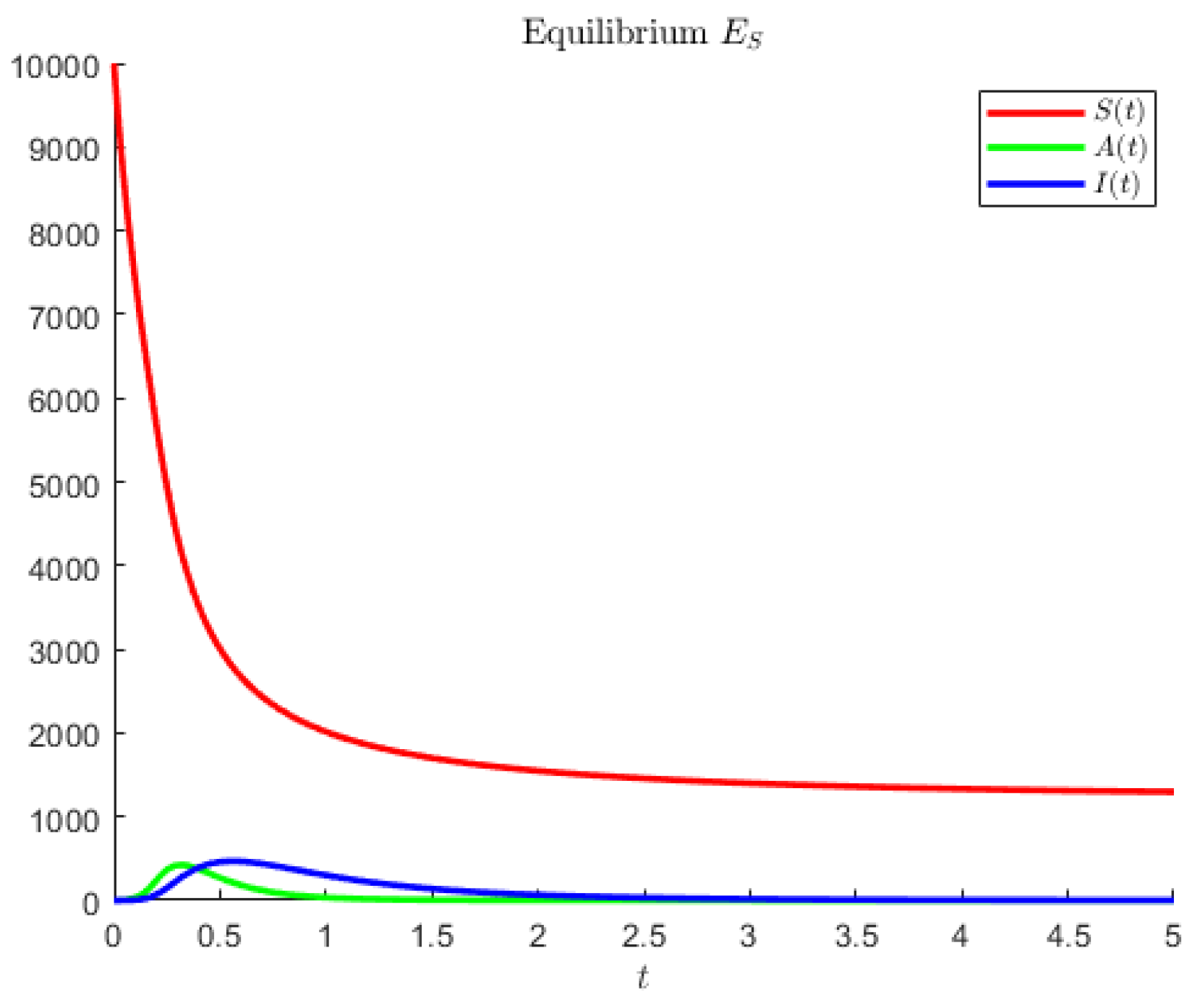
In Figure 1, the disease-free point is attained for model (1) and the hypothetical parameters

$$\begin{array}{c}\hfill \alpha =0.005,\beta =0.006,\mu =0.06,\pi =7,m=0.2,r=0.7.\end{array}$$

(52)

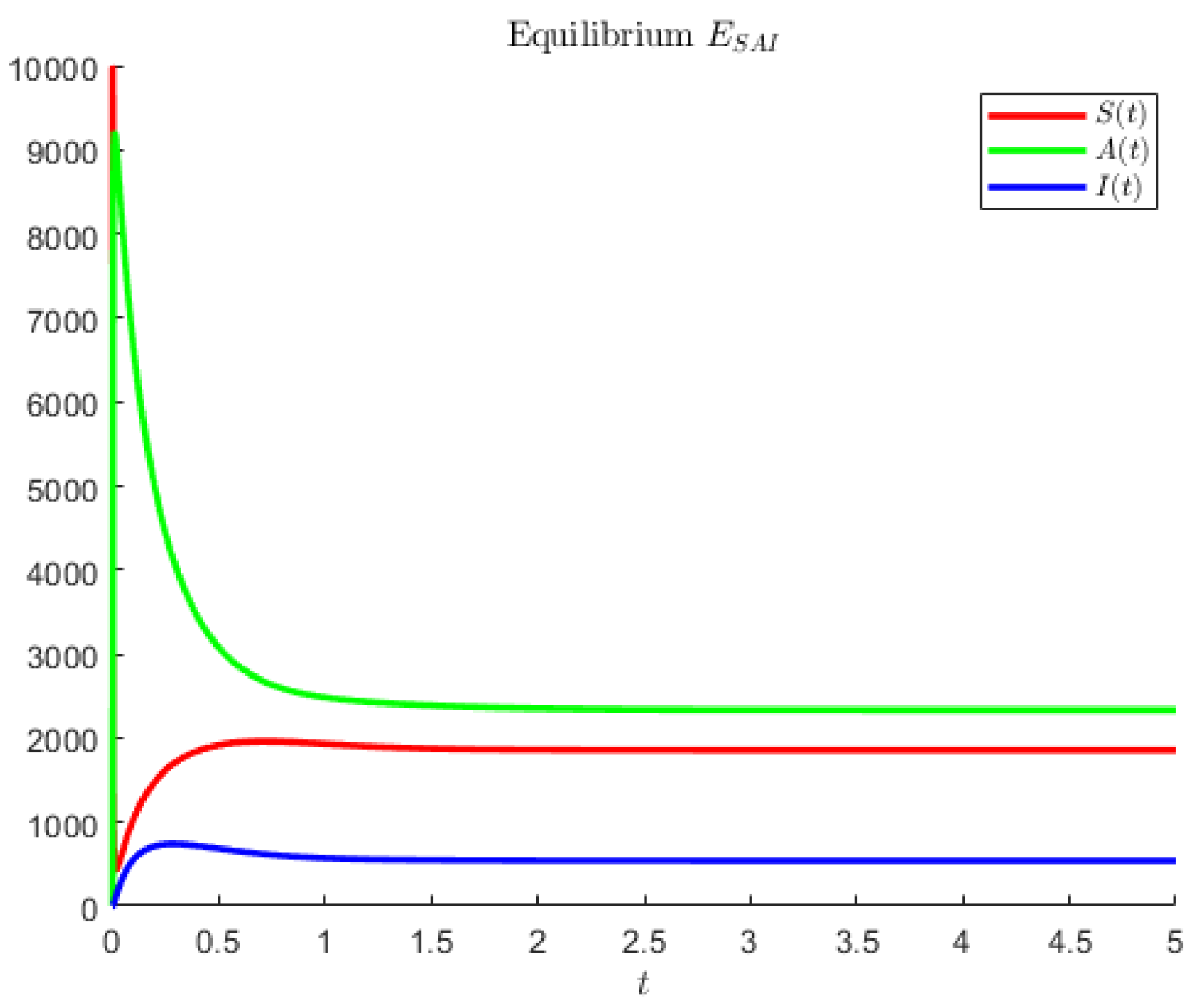
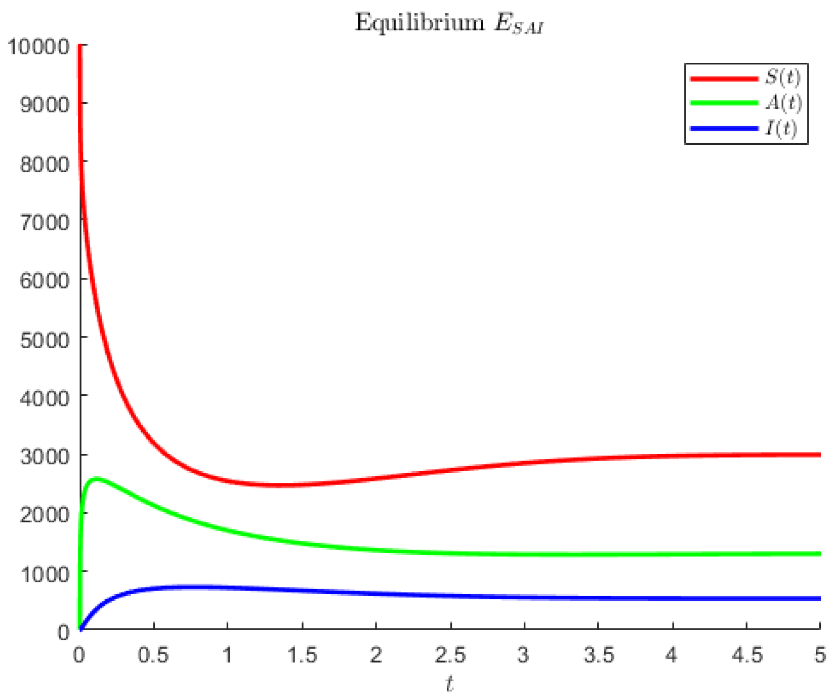
For model (1), in Figure 2, coexistence is obtained using the hypothetical parameter values

$$\begin{array}{c}\hfill \alpha =0.5,\beta =0.6,\mu =0.3,\pi =1,m=0.4,r=3.\end{array}$$

(53)

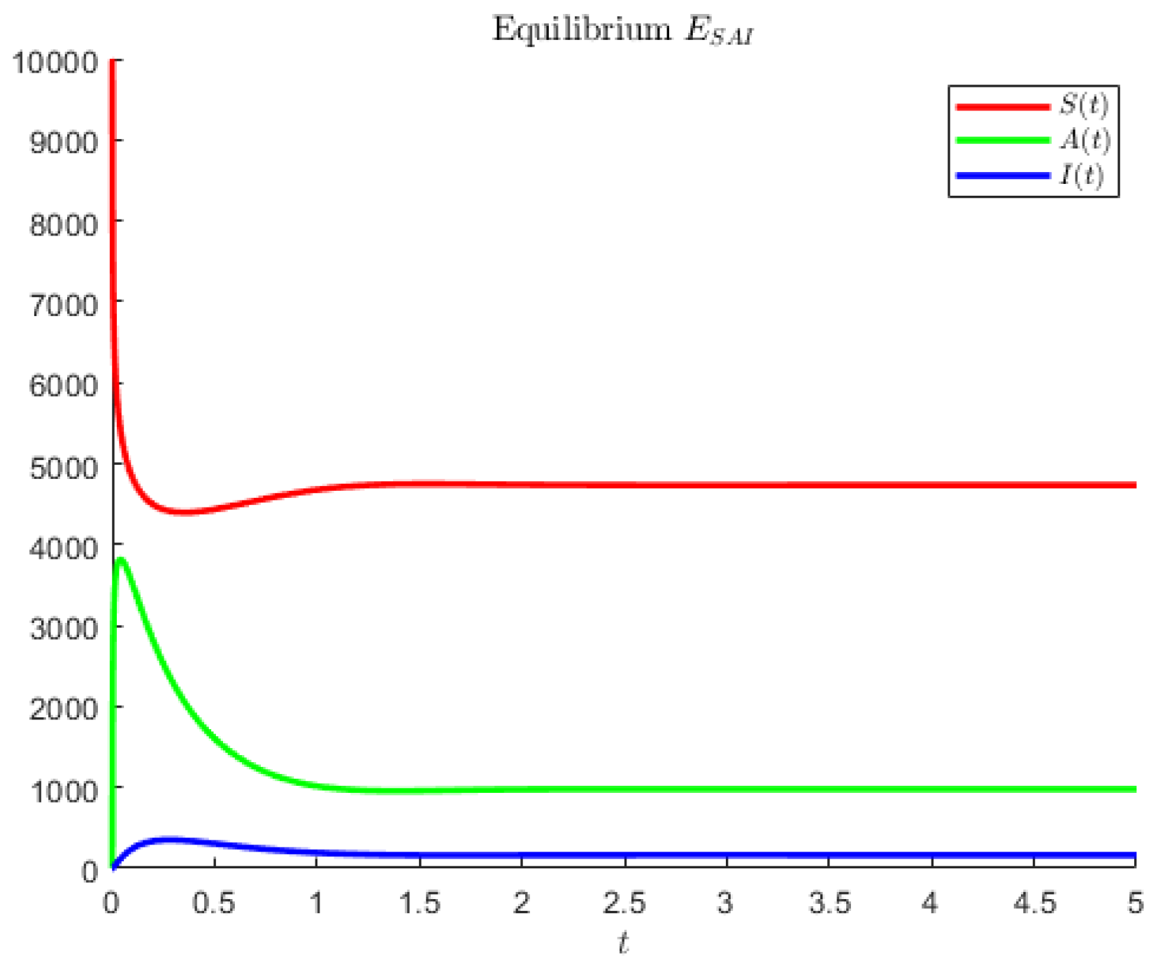
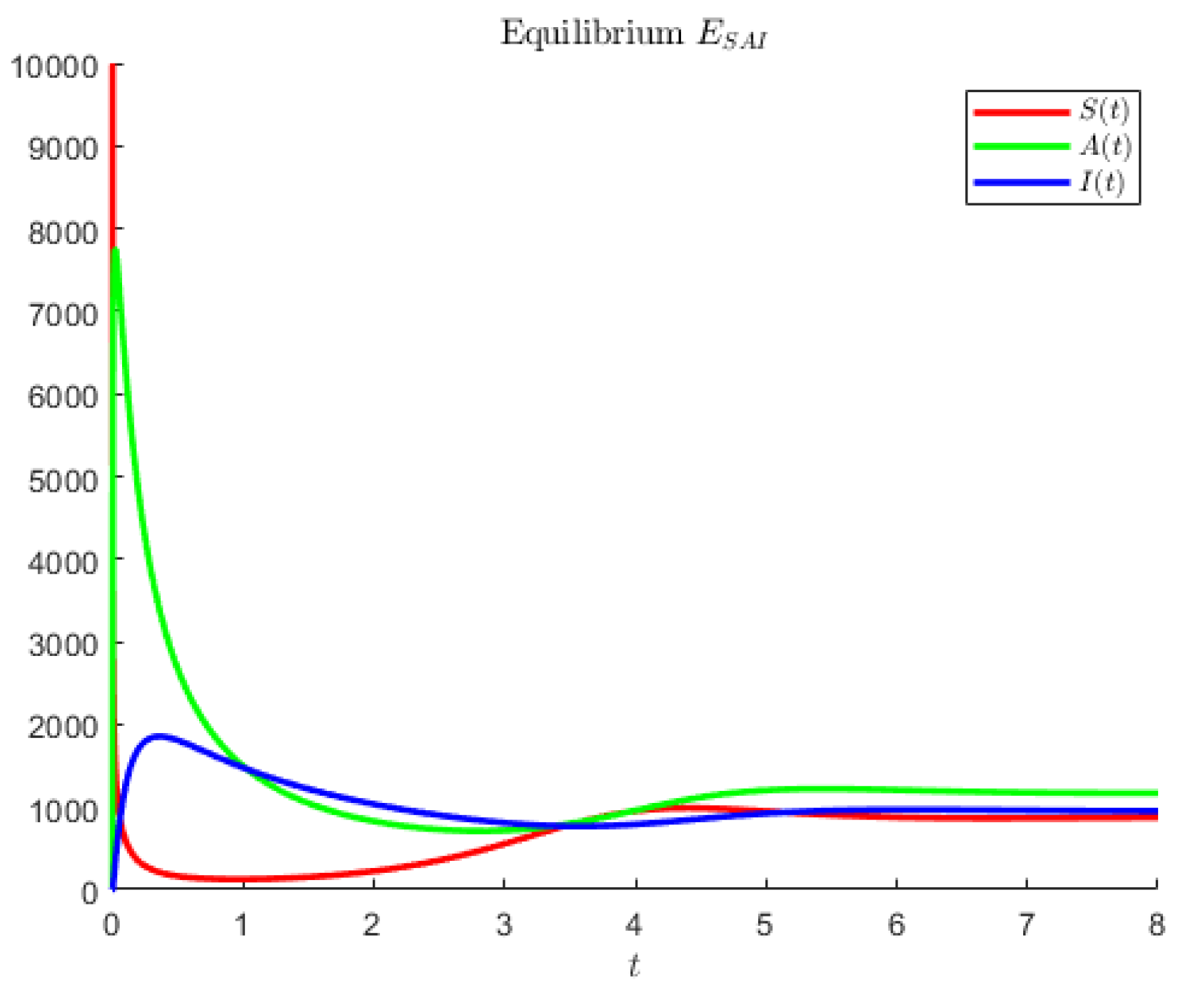
In Figure 3, the hypothetical parameters are

$$\begin{array}{c}\hfill \alpha =0.5,\beta =6,\mu =0.5,\pi =1,m=0.4,r=3.\end{array}$$

(54)

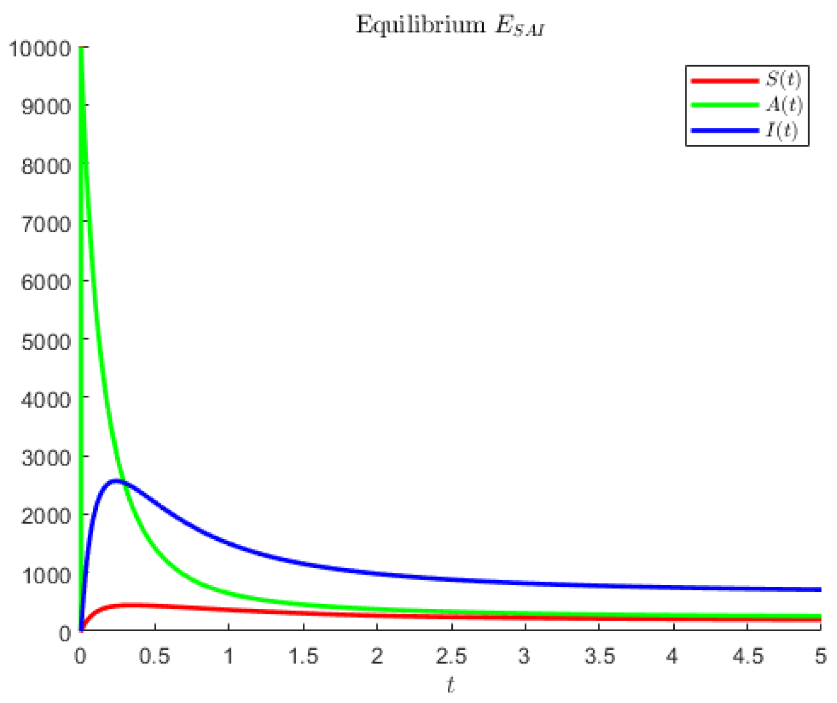
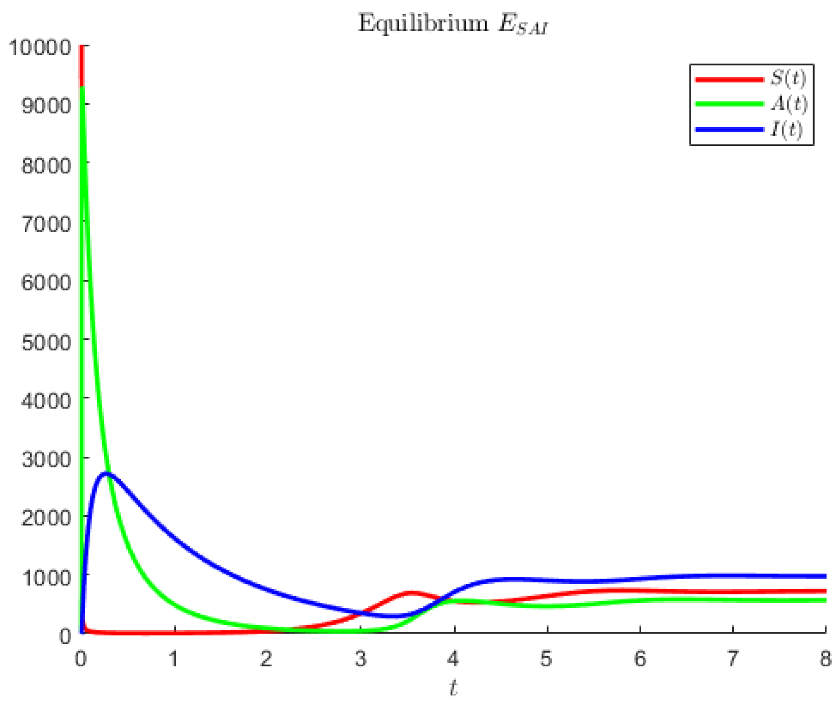
The hypothetical parameters of Figure 4 are

$$\begin{array}{c}\hfill \alpha =0.5,\beta =0.6,\mu =0.3,\pi =4,m=2,r=3.\end{array}$$

(55)

Note that in the former case, the asymptomatics attain the highest value, followed by the susceptibles. In the second case, instead, the disease seems to affect less of the population; the most populated compartment is the one of the susceptibles, followed by the asymptomatic individuals. Figure 4 shows an instance in which the largest population is represented by the symptomatic individuals and the second largest are the asymptomatics.

For the model (23) with vertical transmission, we also show three instances of the endemic equilibrium. The hypothetical parameters of Figure 5 are (51) and

$$\begin{array}{c}\hfill \alpha =0.5,\beta =6,\mu =0.5,\pi =2,m=0.4,r=3,\end{array}$$

(56)

while those hypothetical of Figure 6, in addition to (51), instead being

$$\begin{array}{c}\hfill \alpha =0.5,\beta =0.6,\mu =0.5,\pi =2.5,m=0.4,r=3\end{array}$$

(57)

and those hypothetical parameters for Figure 7, in which the asymptomatics represent the most numerous class, are

$$\begin{array}{c}\hfill \alpha =1.6,\beta =0.6,\mu =0.3,\pi =4,m=0.4,r=3\end{array}$$

(58)

The disease-free point is also attained with the following hypothetical parameters

$$\begin{array}{c}\hfill \alpha =0.5,\beta =0.6,\mu =0.3,\pi =4,m=0.4,r=3.\end{array}$$

The resulting figure is extremely close to Figure 1 and, therefore, it is not shown.

In case of Figure 5, the most populated compartment is the susceptibles, followed by the asymptomatic individuals. In Figure 6, the asymptomatic prevail, followed by the symptomatic individuals, so that in this case the disease has been contracted by a larger proportion of the population. Figure 7 shows, instead, the case in which the asymptomatics represent the largest class.

4. Global Behavior of the Systems

On the basis of the previous results, comparing the feasibility and stability conditions of the various equilibria, we can conjecture the existence of bifurcations relating them. We show analytically their presence, but we can go even further, completely assessing the models behavior.

The first step in this direction is to recall that both models’ trajectories are confined to a compact set, as discussed in Section 2.2 and Section 2.6. In the second place, using Sotomayor’s theorem [22], we show that a chain of transcritical bifurcations ties the various systems’ equilibria.

Model (1) implies that no two such equilibria may appear simultaneously to be stable and feasible, and, therefore, when locally asymptotically stable, they are also globally asymptotically stable. Therefore, these systems move from “disappearance” to the susceptible-only, i.e., disease-free, point, and, finally, to the endemic case.

In order to apply Sotomayor’s theorem, some preliminary calculations are needed. We slightly change our notation, denoting now by $f(S,A,I)={(f_1(S,A,I),f_2(S,A,I),f_3(S,A,I))}^T$ both systems’ (1) and (23) right-hand sides, and by $Df$ their Jacobian.

4.1. Application of Sotomayor’s Theorem for Model (1)

We now determine the second partial derivatives of f with respect to the variables S, A and I, i.e., the elements of $D^{2}f$:

$$\begin{array}{c}\hfill \frac{{\partial }^2{f}_1}{\partial S^2}=-2c_{SS},\frac{{\partial }^2{f}_1}{\partial I^2}=-\frac{2\alpha {\beta }^{2}SA}{{(1+\beta I)}^3},\frac{{\partial }^2{f}_1}{\partial S\partial A}=\frac{{\partial }^2{f}_1}{\partial A\partial S}=-c_{SA}-\frac{\alpha }{1+\beta I},\\ \hfill \frac{{\partial }^2{f}_1}{\partial S\partial I}=\frac{{\partial }^2{f}_1}{\partial I\partial S}=-c_{SI}+\frac{\alpha \beta A}{{(1+\beta I)}^2},\frac{{\partial }^2{f}_1}{\partial A\partial I}=\frac{{\partial }^2{f}_1}{\partial I\partial A}=\frac{\alpha \beta S}{{(1+\beta I)}^2},\frac{{\partial }^2{f}_2}{\partial A^2}=-2c_{AA},\\ \hfill \frac{{\partial }^2{f}_2}{\partial I^2}=\frac{2\alpha {\beta }^{2}SA}{{(1+\beta I)}^3},\frac{{\partial }^2{f}_2}{\partial S\partial A}=\frac{{\partial }^2{f}_2}{\partial A\partial S}=-c_{AS}+\frac{\alpha }{1+\beta I},\frac{{\partial }^2{f}_2}{\partial S\partial I}=\frac{{\partial }^2{f}_2}{\partial I\partial S}=-\frac{\alpha \beta A}{{(1+\beta I)}^2},\\ \hfill \frac{{\partial }^2{f}_2}{\partial A\partial I}=\frac{{\partial }^2{f}_2}{\partial I\partial A}=-c_{AI}-\frac{\alpha \beta S}{{(1+\beta I)}^2},\frac{{\partial }^2{f}_3}{\partial I^2}=-2c_{II},\frac{{\partial }^2{f}_3}{\partial S\partial I}=\frac{{\partial }^2{f}_3}{\partial I\partial S}=-c_{IS},\\ \hfill \frac{{\partial }^2{f}_3}{\partial A\partial I}=\frac{{\partial }^2{f}_3}{\partial I\partial A}=-c_{IA},\frac{{\partial }^2{f}_1}{\partial A^2}=\frac{{\partial }^2{f}_2}{\partial S^2}=\frac{{\partial }^2{f}_3}{\partial S^2}=\frac{{\partial }^2{f}_3}{\partial A^2}=\frac{{\partial }^2{f}_3}{\partial S\partial A}=\frac{{\partial }^2{f}_3}{\partial A\partial S}=0.\end{array}$$

Furthermore, by differentiating the components of f with respect to r, we find

$$f_r={\left[\frac{\partial f_1}{\partial r},\frac{\partial f_2}{\partial r},\frac{\partial f_3}{\partial r}\right]}^T={\left[S+A,0,0\right]}^T,$$

whose Jacobian, differentiating with respect to the variables S, A and I, is

$$D{f}_r=\left[\begin{array}{ccc}1& 1& 0\\ 0& 0& 0\\ 0& 0& 0\end{array}\right].$$

(59)

4.1.1. Transcritical Bifurcation $E_0\to E_S$

Consider the equilibrium point $E_0$ and choose r as the bifurcation parameter.

Evaluating the Jacobian at the equilibrium $E_0$, we obtain

$$J=Df\left(E_0,r\right)=\left[\begin{array}{ccc}r-m& m& 0\\ 0& -m-\pi & 0\\ 0& \pi & -m-\mu \end{array}\right],$$

having the eigenvalues ${\lambda }_1=r-m$, ${\lambda }_2=-m-\pi$ and ${\lambda }_3=-m-\mu$; thus, two eigenvalues have a negative real part and the first one vanishes by taking as the critical bifurcation value

$$r_0=m.$$

(60)

Its right v and left w eigenvectors corresponding to the zero eigenvalue are, therefore

$$v={[1,0,0]}^T,w={\left[\frac{m+\pi }{m},1,0\right]}^T.$$

The only nonvanishing terms in $D^{2}f\left(E_0,m\right)$ are

$$\begin{array}{c}\hfill \frac{{\partial }^2{f}_1}{\partial S^2}=-2c_{SS},\frac{{\partial }^2{f}_1}{\partial S\partial A}=\frac{{\partial }^2{f}_1}{\partial A\partial S}=-c_{SA}-\alpha ,\frac{{\partial }^2{f}_1}{\partial S\partial I}=\frac{{\partial }^2{f}_1}{\partial I\partial S}=-c_{SI},\\ \hfill \frac{{\partial }^2{f}_2}{\partial A^2}=-2c_{AA},\frac{{\partial }^2{f}_2}{\partial S\partial A}=\frac{{\partial }^2{f}_2}{\partial A\partial S}=-c_{AS}+\alpha ,\frac{{\partial }^2{f}_2}{\partial A\partial I}=\frac{{\partial }^2{f}_2}{\partial I\partial A}=-c_{AI},\\ \hfill \frac{{\partial }^2{f}_3}{\partial I^2}=-2c_{II},\frac{{\partial }^2{f}_3}{\partial S\partial I}=\frac{{\partial }^2{f}_3}{\partial I\partial S}=-c_{IS},\frac{{\partial }^2{f}_3}{\partial A\partial I}=\frac{{\partial }^2{f}_3}{\partial I\partial A}=-c_{IA}.\end{array}$$

(61)

Furthermore, recalling (59), we have

$$f_r\left(E_0,m\right)={\left[0,0,0\right]}^T,D{f}_r\left(E_0,m\right)=D{f}_r.$$

Finally, the components of $D^{2}f\left(E_0,m\right)(v,v)$ are

$$D^2{f}_1\left(E_0,m\right)(v,v)=-2c_{SS}{v}_1^2-2(c_{SA}+\alpha )v_1{v}_2-2c_{SI}{v}_1{v}_3,$$

$$D^2{f}_2\left(E_0,m\right)(v,v)=-2c_{AA}{v}_2^2-2(c_{AS}-\alpha )v_1{v}_2-2c_{AI}{v}_2{v}_3,$$

$$D^2{f}_3\left(E_0,m\right)(v,v)=-2c_{II}{v}_3^2-2c_{IS}{v}_1{v}_3-2c_{IA}{v}_2{v}_3.$$

Thus, the three conditions required by Sotomayor’s Theorem for a transcritical bifurcation are met; indeed

$$\begin{array}{c}\hfill w^T{f}_r\left(E_0,m\right)=0,w^T\left[D{f}_r\left(E_0,m\right)v\right]=w_1{v}_1=\frac{m+\pi }{m}\ne 0,\\ \hfill w^T\left[D^{2}f\left(E_0,m\right)(v,v)\right]=-2c_{SS}{w}_1{v}_1^2=-\frac{2c_{SS}(m+\pi )}{m}\ne 0.\end{array}$$

4.1.2. Transcritical Bifurcation $E_S\to E_{SAI}$

Now consider the $E_S$ and choose r as the bifurcation parameter.

The Jacobian evaluated at $E_S$ is

$$\begin{array}{c}\hfill J=Df\left(E_S,r\right)=\left[\begin{array}{ccc}-{\displaystyle \frac{c_{SS}(m+\pi )}{\alpha -c_{AS}}}& J_{1,2}& -{\displaystyle \frac{c_{IS}(m+\pi )}{\alpha -c_{AS}}}\\ 0& J_{2,2}& 0\\ 0& \pi & -{\displaystyle \frac{(\alpha -c_{AS})(m+\mu )+c_{IS}(m+\pi )}{\alpha -c_{AS}}}\end{array}\right],\end{array}$$

with

$$J_{1,2}={\displaystyle \frac{(c_{SS}-c_{AS}-c_{SA})m+(c_{SS}-c_{SA}-\alpha )\pi }{\alpha -c_{AS}}},J_{2,2}=-m-\pi +(\alpha -c_{AS}){\displaystyle \frac{r-m}{c_{SS}}}.$$

Its eigenvalues are

$${\lambda }_1=-{\displaystyle \frac{c_{SS}(m+\pi )}{\alpha -c_{AS}}},{\lambda }_2=J_{22},{\lambda }_3=-{\displaystyle \frac{(\alpha -c_{AS})(m+\mu )+c_{IS}(m+\pi )}{\alpha -c_{AS}}}.$$

Now, ${\lambda }_2$ vanishes by choosing the critical value

$$r^{†}=m+{\displaystyle \frac{c_{SS}(m+\pi )}{\alpha -c_{AS}}},$$

(62)

while the remaining ones are negative, if $\alpha >c_{AS}$; or the first one is positive, if $\alpha <c_{AS}$. The left eigenvector is $w={\left[0,1,0\right]}^T$, while the right one is

$$v=\left[\begin{array}{c}\frac{1}{c_{SS}(m+\pi )}\left(\frac{((c_{SS}-c_{AS}-c_{SA})m+(c_{SS}-c_{SA}-\alpha )\pi )((\alpha -c_{AS})(m+\mu )+c_{IS}(m+\pi ))}{(\alpha -c_{AS})\pi }-c_{SI}(m+\pi )\right)\\ {\displaystyle \frac{(\alpha -c_{AS})(m+\mu )+c_{IS}(m+\pi )}{(\alpha -c_{AS})\pi }}\\ 1\end{array}\right].$$

Recalling (59), we further have

$$f_r\left(E_S,r^{†}\right)={\left[{\displaystyle \frac{m+\pi }{\alpha -c_{AS}}},0,0\right]}^T,D{f}_r\left(E_S,r^{†}\right)=D{f}_r.$$

However, in spite of having $w^T{f}_r\left(E_S,r^{†}\right)=0$, Sotomayor’s Theorem is inconclusive because the last condition is not satisfied, namely $w^T\left[D{f}_r\left(E_S,r^{†}\right)v\right]=0$.

Remark 1. 

This calculation is very interesting, because in spite of the fact that the analysis is undecided concerning the existence of the transcritical bifurcation, the simulations below will show that it does indeed take place. Thus, it is an example of the fact that the conditions in Sotomayor’s Theorem are sufficient but not necessary.

4.2. Application of Sotomayor’s Theorem for Model (23)

The proof follows pretty much the one of model (1). We outline only the basic changes. Once again, we use the same notation for f and $Df$, which, here, denote the right hand side and the Jacobian of (23). The only changes in the Jacobian are the elements

$$\frac{\partial f_1}{\partial A}=-c_{SA}S-\frac{\alpha S}{1+\beta I},\frac{\partial f_2}{\partial A}=r-m-2c_{AA}A-c_{AS}S-c_{AI}I+\frac{\alpha S}{1+\beta I}-\pi .$$

It further turns out that $D^{2}f$ is the same as the one of model (1). Here, instead, we find

$$f_r={\left[\frac{\partial f_1}{\partial r},\frac{\partial f_2}{\partial r},\frac{\partial f_3}{\partial r}\right]}^T={\left[S,A,0\right]}^T,$$

whose Jacobian—differentiating with respect to the variables S, A and I—is now

$$D{f}_r=\left[\begin{array}{ccc}1& 0& 0\\ 0& 1& 0\\ 0& 0& 0\end{array}\right].$$

4.2.1. Transcritical Bifurcation $E_0\to E_S$

We consider the equilibrium point $E_0$ and we choose r as the bifurcation parameter.

By evaluating the Jacobian, we obtain

$$J=Df\left(E_0,r\right)=\left[\begin{array}{ccc}r-m& 0& 0\\ 0& -\pi & 0\\ 0& \pi & -m-\mu \end{array}\right],$$

having the eigenvalues ${\lambda }_1=r-m$, ${\lambda }_2=-\pi$ and ${\lambda }_3=-m-\mu$, two of them being negative. The first one vanishes by taking, again, $r_0=m$ as in (60), the same the critical bifurcation threshold as for model (1). The left and right eigenvectors are, respectively

$$v={[1,0,0]}^T,w={\left[1,0,0\right]}^T.$$

The elements of $D^{2}f\left(E_0,r_0\right)$ are the same as the first model, because $D^{2}f$ is the same; consequently, also, are the components of

$$D^{2}f\left(E_0,r_0\right)(v,v)={\left[D^2{f}_1\left(E_0,r_0\right)(v,v),D^2{f}_2\left(E_0,r_0\right)(v,v),D^2{f}_3\left(E_0,r_0\right)(v,v)\right]}^T.$$

Furthermore, recalling (59), we have

$$f_r\left(E_0,r_0\right)={\left[0,0,0\right]}^T,D{f}_r\left(E_0,r_0\right)=D{f}_r.$$

Thus, the three conditions required by Sotomayor’s Theorem are met; indeed

$$\begin{array}{c}\hfill w^T{f}_r\left(E_0,m\right)=0,w^T\left[D{f}_r\left(E_0,m\right)v\right]=w_1{v}_1=1\ne 0,\\ \hfill w^T\left[D^{2}f\left(E_0,m\right)(v,v)\right]=-2c_{SS}{w}_1{v}_1^2=-2c_{SS}\ne 0.\end{array}$$

Hence, at $r=r_0=m$, there is a transcritical bifurcation for which $E_0$ becomes $E_S$.

4.2.2. Transcritical Bifurcation $E_S\to E_{SAI}$

We consider the equilibrium point $E_S$ and we choose r as the bifurcation parameter. From the evaluation of the Jacobian, for

$$c_{AS}\ne c_{SS}+\alpha$$

(63)

we obtain

$$J=Df\left(E_S,r\right)=\left[\begin{array}{ccc}-{\displaystyle \frac{c_{SS}\pi }{c_{SS}-c_{AS}+\alpha }}& -{\displaystyle \frac{(c_{AS}+\alpha )\pi }{c_{SS}-c_{AS}+\alpha }}& -{\displaystyle \frac{c_{IS}\pi }{c_{SS}-c_{AS}+\alpha }}\\ 0& J_{22}& 0\\ 0& \pi & -m-\mu -{\displaystyle \frac{c_{IS}\pi }{c_{SS}-c_{AS}+\alpha }}\end{array}\right],$$

having the eigenvalues

$${\lambda }_1=-{\displaystyle \frac{c_{SS}\pi }{c_{SS}-c_{AS}+\alpha }},{\lambda }_2=J_{22},{\lambda }_3=-m-\mu -{\displaystyle \frac{c_{IS}\pi }{c_{SS}-c_{AS}+\alpha }}.$$

The second eigenvalue vanishes by taking as the critical bifurcation threshold

$$r^{‡}=m+{\displaystyle \frac{c_{SS}\pi }{c_{SS}-c_{AS}+\alpha }}>m,$$

(64)

the latter inequality following by requiring ${\lambda }_1<0$. Note that $r^{†}$ for model (1) and $r^{‡}$ for model (23) differ; compare (62) and (64). The left and right eigenvectors are, respectively

$$v=\left[\begin{array}{c}{\displaystyle \frac{c_{SI}}{c_{SS}}}-{\displaystyle \frac{c_{AS}+\alpha }{c_{SS}}}\left({\displaystyle \frac{m+\mu }{\pi }}+{\displaystyle \frac{c_{IS}}{c_{SS}-c_{AS}+\alpha }}\right)\\ {\displaystyle \frac{m+\mu }{\pi }}+{\displaystyle \frac{c_{IS}}{c_{SS}-c_{AS}+\alpha }}\\ 1\end{array}\right],w={\left[0,1,0\right]}^T.$$

The nonvanishing elements of $D^{2}f\left(E_S,r^{‡}\right)$ are exactly those of (61) with the exception of

$$\frac{{\partial }^2{f}_1}{\partial A\partial I}=\frac{{\partial }^2{f}_1}{\partial I\partial A}=\frac{\alpha \beta \pi }{c_{SS}-c_{AS}+\alpha },\frac{{\partial }^2{f}_2}{\partial A\partial I}=\frac{{\partial }^2{f}_2}{\partial I\partial A}=-c_{AI}-\frac{\alpha \beta \pi }{c_{SS}-c_{AS}+\alpha },\frac{{\partial }^2{f}_3}{\partial I^2}=-2c_{II}.$$

Further, recalling once again (59), we have

$$f_r\left(E_S,r^{‡}\right)={\left[{\displaystyle \frac{\pi }{c_{SS}-c_{AS}+\alpha }},0,0\right]}^T,D{f}_r\left(E_S,r^{‡}\right)=D{f}_r.$$

Finally, the components of

$$D^{2}f\left(E_S,r^{‡}\right)(v,v)={\left[D^2{f}_1\left(E_S,r^{‡}\right)(v,v),D^2{f}_2\left(E_S,r^{‡}\right)(v,v),D^2{f}_3\left(E_S,r^{‡}\right)(v,v)\right]}^T$$

are

$$\begin{array}{c}\hfill D^2{f}_1\left(E_S,r^{‡}\right)(v,v)=-2c_{SS}{v}_1^2-2(c_{SA}+\alpha )v_1{v}_2-2c_{SI}{v}_1{v}_3+\frac{2\alpha \beta \pi }{c_{SS}-c_{AS}+\alpha }{v}_2{v}_3,\\ \hfill D^2{f}_2\left(E_S,r^{‡}\right)(v,v)=-2c_{AA}{v}_2^2-2(c_{AS}-\alpha )v_1{v}_2-2\left(c_{IA}+\frac{\alpha \beta \pi }{c_{SS}-c_{AS}+\alpha }\right)v_2{v}_3,\\ \hfill D^2{f}_3\left(E_S,r^{‡}\right)(v,v)=-2c_{II}{v}_3^2-2c_{IS}{v}_1{v}_3-2c_{IA}{v}_2{v}_3.\end{array}$$

The first condition required to use Sotomayor’s Theorem is $w^T{f}_r\left(E_S,r^{‡}\right)=0$. We would also need the nonvanishing of the following quantities:

$$\begin{array}{c}\hfill w^T\left[D{f}_r\left(E_S,r^{‡}\right)v\right]=v_2=\frac{m+\mu }{\pi }+\frac{c_{IS}}{c_{SS}-c_{AS}+\alpha },\end{array}$$

(65)

$$\begin{array}{c}\hfill w^T\left[D^{2}f\left(E_S,r^{‡}\right)(v,v)\right]=D^2{f}_2\left(E_S,r^{‡}\right)(v,v)=-2c_{AA}{\left(\frac{m+\mu }{\pi }+\frac{c_{IS}}{c_{SS}-c_{AS}+\alpha }\right)}^2\\ \hfill -2(c_{AS}-\alpha )\left(\frac{c_{SI}}{c_{SS}}-\frac{c_{AS}+\alpha }{c_{SS}}\left(\frac{m+\mu }{\pi }+\frac{c_{IS}}{c_{SS}-c_{AS}+\alpha }\right)\right)\left(\frac{m+\mu }{\pi }+\frac{c_{IS}}{c_{SS}-c_{AS}+\alpha }\right)\\ \hfill -2\left(c_{IA}+\frac{\alpha \beta \pi }{c_{SS}-c_{AS}+\alpha }\right)\left(\frac{m+\mu }{\pi }+\frac{c_{IS}}{c_{SS}-c_{AS}+\alpha }\right).\end{array}$$

(66)

The first one is satisfied and shows that either a transcritical or a pitchfork bifurcation is possible. The remaining ones are needed for a transcritical bifurcation. Thus, if these quantities are different from 0 for $r=r^{‡}$, there is a transcritical bifurcation from $E_S$ to $E_{SAI}$.

In case (66) vanishes, we further investigate the situation. We can observe that (65) is zero if and only if

$$\pi =-\frac{(m+\mu )(c_{SS}-c_{AS}+\alpha )}{c_{IS}},$$

(67)

while (66) is zero if and only if either (67) holds or

$$\begin{array}{c}{c}_{AA}=\frac{\pi (c_{SS}-c_{AS}+\alpha )}{(m+\mu )(c_{SS}-c_{AS}+\alpha )+\pi c_{IS}}\hfill \\ \hfill \times \left\{(\alpha -c_{AS})\left[\frac{c_{SI}}{c_{SS}}-\frac{c_{AS}+\alpha }{c_{SS}}\left(\frac{m+\mu }{\pi }+\frac{c_{IS}}{c_{SS}-c_{AS}+\alpha }\right)\right]-c_{AI}-\frac{\alpha \beta \pi }{c_{SS}-c_{AS}+\alpha }\right\},\end{array}$$

(68)

and, in this second case, we must assume

$$\pi \ne -\frac{(m+\mu )(c_{SS}-c_{AS}+\alpha )}{c_{IS}}.$$

(69)

Now, because $w={[0,1,0]}^T$, the third derivatives simplify, namely

$$w^T\left[D^{3}f(E_S,r^{‡})(v,v,v)\right]=D^3{f}_2(E_S,r^{‡})(v,v,v).$$

The only nonvanishing third partial derivatives of $f_2$ are

$$\frac{{\partial }^3{f}_2}{\partial I^3}=-\frac{6\alpha {\beta }^{3}SA}{{(1+\beta I)}^4},$$

$$\frac{{\partial }^3{f}_2}{\partial I^2\partial S}=\frac{{\partial }^3{f}_2}{\partial S\partial I^2}=\frac{{\partial }^3{f}_2}{\partial I\partial S\partial I}=\frac{2\alpha {\beta }^{2}A}{{(1+\beta I)}^3},\frac{{\partial }^3{f}_2}{\partial I^2\partial A}=\frac{{\partial }^3{f}_2}{\partial A\partial I^2}=\frac{{\partial }^3{f}_2}{\partial I\partial A\partial I}=\frac{2\alpha {\beta }^{2}S}{{(1+\beta I)}^3}$$

and

$$\begin{array}{c}\hfill \frac{{\partial }^3{f}_2}{\partial S\partial A\partial I}=\frac{{\partial }^3{f}_2}{\partial S\partial I\partial A}=\frac{{\partial }^3{f}_2}{\partial A\partial S\partial I}=\frac{{\partial }^3{f}_2}{\partial A\partial I\partial S}=\frac{{\partial }^3{f}_2}{\partial I\partial S\partial A}=\frac{{\partial }^3{f}_2}{\partial I\partial A\partial S}=-\frac{\alpha \beta }{{(1+\beta I)}^2}.\end{array}$$

Of these, upon evaluation at $(E_S,r^{‡})$, the only nonvanishing ones are those in the last two groups, namely

$$\frac{{\partial }^3{f}_2(E_S,r^{‡})}{\partial I^2\partial A}=\frac{{\partial }^3{f}_2(E_S,r^{‡})}{\partial A\partial I^2}=\frac{{\partial }^3{f}_2(E_S,r^{‡})}{\partial I\partial A\partial I}=\frac{2\alpha {\beta }^2\pi }{c_{SS}-c_{AS}+\alpha }$$

and

$$\begin{array}{c}\hfill \frac{{\partial }^3{f}_2(E_S,r^{‡})}{\partial S\partial A\partial I}=\frac{{\partial }^3{f}_2(E_S,r^{‡})}{\partial S\partial I\partial A}=\frac{{\partial }^3{f}_2(E_S,r^{‡})}{\partial A\partial S\partial I}=\frac{{\partial }^3{f}_2(E_S,r^{‡})}{\partial A\partial I\partial S}\\ \hfill =\frac{{\partial }^3{f}_2(E_S,r^{‡})}{\partial I\partial S\partial A}=\frac{{\partial }^3{f}_2(E_S,r^{‡})}{\partial I\partial A\partial S}=-\alpha \beta .\end{array}$$

Consequently

$$\begin{array}{c}\hfill w^T\left[D^{3}f(E_S,r^{‡})(v,v,v)\right]=D^3{f}_2(E_S,r^{‡})(v,v,v)=\sum _{j_1,j_2,j_3=1}^3\frac{{\partial }^3{f}_2(E_S,r^{‡})}{\partial x_{j_1}\partial x_{j_2}\partial x_{j_3}}{v}_{j_1}{v}_{j_2}{v}_{j_3}\\ \hfill =3\frac{{\partial }^3{f}_2(E_S,r^{‡})}{\partial A\partial I^2}{v}_2{v}_3^2+6\frac{{\partial }^3{f}_2(E_S,r^{‡})}{\partial S\partial A\partial I}{v}_1{v}_2{v}_3=6\alpha \beta v_2{v}_3\left(\frac{\beta \pi }{c_{SS}-c_{AS}+\alpha }{v}_3-v_1\right).\end{array}$$

Substituting into this expression the components of v we explicitly have

$$\begin{array}{c}{w}^T\left[D^{3}f(E_S,r^{‡})(v,v,v)\right]=6\alpha \beta \left({\displaystyle \frac{m+\mu }{\pi }}+{\displaystyle \frac{c_{IS}}{c_{SS}-c_{AS}+\alpha }}\right)\hfill \\ \hfill \times \left[\frac{\beta \pi }{c_{SS}-c_{AS}+\alpha }-{\displaystyle \frac{c_{SI}}{c_{SS}}}+{\displaystyle \frac{c_{AS}+\alpha }{c_{SS}}}\left({\displaystyle \frac{m+\mu }{\pi }}+{\displaystyle \frac{c_{IS}}{c_{SS}-c_{AS}+\alpha }}\right)\right].\end{array}$$

(70)

Still assuming (63),we can observe that (70) is zero if and only if (67) holds or, alternatively

$$\beta =\frac{c_{SI}{c}_{SS}\pi -(c_{AS}-\alpha )c_{SI}\pi -(m+\mu )(c_{AS}+\alpha )(c_{SS}-c_{AS}+\alpha )-c_{IS}{c}_{SS}\pi }{c_{SS}{\pi }^2}.$$

(71)

In summary, for the case (63), since Sotomayor’s Theorem gives only sufficient conditions, we cannot conclude anything about the bifurcation from $E_S$ for $r=r^{‡}$ being a saddle-node. Instead, a sufficient condition for a transcritical bifurcation to exist is that the conditions (67) and (68) are both not satisfied; alternatively, a pitchfork bifurcation occurs if (67) and (71) are not satisfied but (68) is verified.

We, finally, also investigate the case for which (63) does not hold, i.e., $c_{SS}-c_{AS}+\alpha =0$. The Jacobian evaluated at $E_S$ gives ${\widehat{J}}_{22}=-\pi$. Taking now $\pi$ as the bifurcation parameter, with threshold value ${\pi }_0=0$, we find the right and left eigenvectors $v={[v_1,v_2,0]}^T$$w={[0,1,0]}^T$, with

$$v_1=-\frac{c_{SS}}{c_{SA}+\alpha }<0,v_2=1>0.$$

In addition, calculating the derivative with respect to the bifurcation parameter, $f_{\pi }={[0,-A,A]}^T$ so that $f_{\pi }(E_S,\pi )={[0,0,0]}^T$ and $w^T{f}_{\pi }(E_S,\pi )=0$. Upon evaluation of the Jacobian $D{f}_{\pi }$, it also follows that $w^{T}D{f}_{\pi }(E_S,\pi )v={[0,-1,0]}^{T}v=-v_2>0$. Since $w_1=w_3=0$, it is enough to calculate just the partial derivatives of the second component of f:

$$w^T{D}^{2}f(v,v)=\frac{{\partial }^2{f}_2}{\partial S^2}{v}_1^2+2\frac{{\partial }^2{f}_2}{\partial A\partial S}{v}_1{v}_2+\frac{{\partial }^2{f}_2}{\partial A^2}{v}_2^2=-2c_{AS}{v}_1{v}_2-2c_{AA}A{v}_2^2$$

so that

$$w^T{D}^2{f(v,v)|}_{(E_S,\pi )}=-2c_{AS}{v}_1{v}_2>0$$

and, therefore, there is also no transcritical bifurcation in this case.

Remark 2. 

Note that if we try to apply the same technique to the situation $\alpha -c_{AS}=0$ for (1), we obtain $J_{22}=-m-\pi$, so that in this case the threshold value for the bifurcation parameter π would be negative, ${\pi }_0^{\left(1\right)}=-m<0$, and, therefore, not biologically feasible.

4.3. Numerical Simulations for the Bifurcations

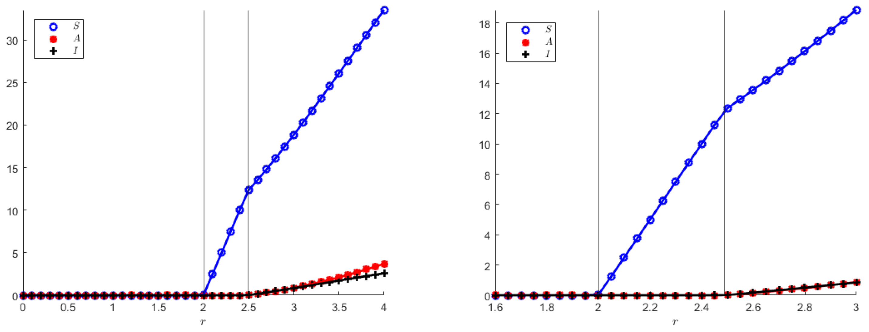
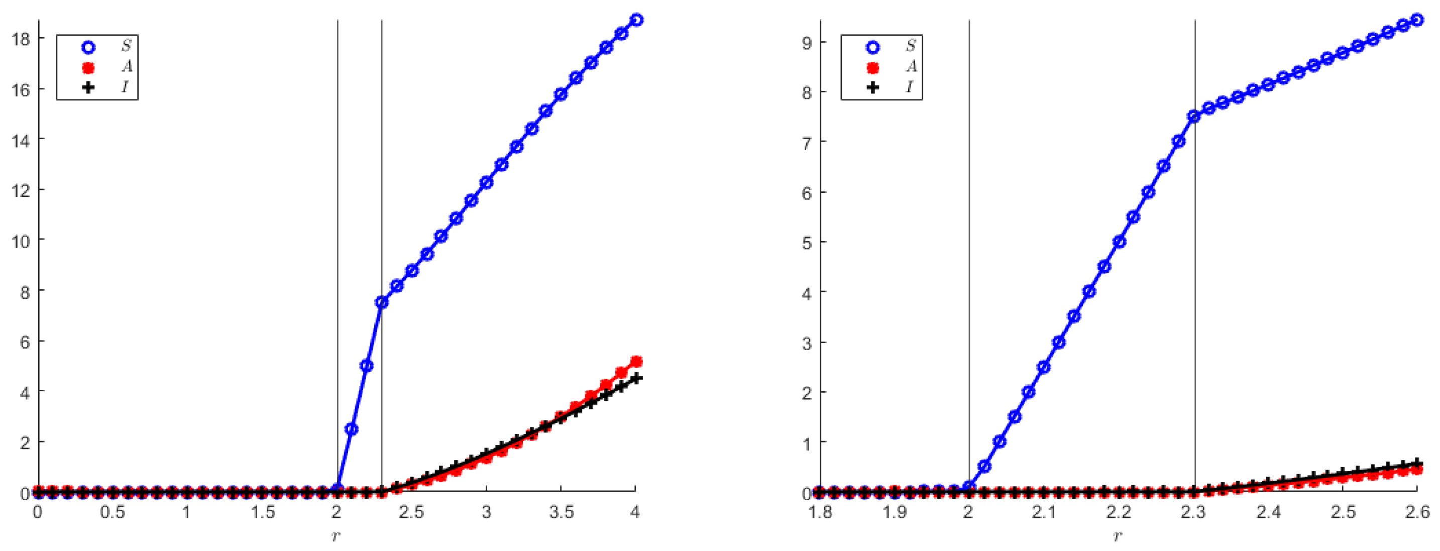
In addition, we also show numerically the two transcritical bifurcation diagrams, indicating in particular that the coexistence equilibrium in both models originates from the disease-free equilibrium, which, in turn, arises from the origin when the population reproduction rate overcomes its mortality rate, as it also appears from the theoretical analysis. Note that Figure 8 and Figure 9 qualitatively appear to be the same, but their vertical axes differ quite a bit.

The transcritical bifurcation parameters for both model (1) and (23), still using (55) are:

$$\begin{array}{c}\hfill c_{SS}=0.04,c_{AA}=0.05,c_{II}=0.06,c_{SA}=0.08,c_{SI}=0.03,\\ \hfill c_{AS}=0.01,c_{AI}=0.02,c_{IS}=0.09,c_{IA}=0.07.\end{array}$$

(72)

5. Discussion

This investigation has been prompted by the recent COVID-19 pandemic, in which, at least at its outbreak, the role of asymptomatic individuals was apparently fundamental. We consider the general population response to such an event. The now classical Capasso–Serio model [9] was the first to encompass this feature. Although more generally formulated, it also contains three compartments: susceptibles, infected and removed.

The specific form for the model [9] that we adopt in our simulations for comparison purposes is the following:

$$\begin{array}{ccc}\hfill \frac{dS}{dt}& =& -\frac{\alpha SI}{1+\beta I^2},\hfill \\ \hfill \frac{dI}{dt}& =& \frac{\alpha SI}{1+\beta I^2}-\gamma I,\hfill \\ \hfill \frac{dR}{dt}& =& \gamma I.\hfill \end{array}$$

(73)

As already mentioned in the Introduction, the SAI models (1) and (23) proposed here from the epidemiological viewpoint are an extension of the classical SI model or as an SIR model in which R stands for removed rather than recovered. Since, in the SI case, removed do not appear, in a sense (1) and (23) share its properties. Introducing the asymptomatics A in (1) and (23), the infected are split among A and symptomatics I. System (1) or (23) can be compared with the Capasso–Serio model by means of the following matches:

$$\begin{array}{c}\hfill S:\left(1\right)\to S:\left(73\right),\left(\mathrm{the}\mathrm{susceptible}\mathrm{classes}\right)\\ \hfill A:\left(1\right)\to I:\left(73\right),\left(\mathrm{the}\mathrm{classes}\mathrm{that}\mathrm{can}\mathrm{transmit}\mathrm{the}\mathrm{disease}\right)\\ \hfill I:\left(1\right)\to R:\left(23\right),\left(\mathrm{removed}\mathrm{from}\mathrm{circulation}\mathrm{and}\mathrm{unable}\mathrm{to}\mathrm{transmit}\mathrm{the}\mathrm{disease}\right).\end{array}$$

In (1) and (23), I are recognized as disease carriers. In order to possibly not get the disease, the susceptibles take the size of symptomatic I as an index by which to measure the reduction in their contacts with all other individuals. In (73), instead, both I and R are recognized as disease carriers, but R are isolated and cannot produce new cases of the disease. Here, the contact reductions are based on the size of the infected class I. Both I for (1) and (23) as well as R for (73), represent sinks for the dynamical system. In the comparison between (1) (or (23)) and (73), only the people that can spread the disease are relevant, respectively, A and I. However, the important point is that the people can only react to the infected they see, i.e., I in both models. Note, indeed, that in spite of the above matching among compartments, we cannot completely identify the asymptomatics A of our case with the infected in [9], nor our symptomatic individuals I with the removed of [9], because the “fear” response function in our model depends inversely on symptomatics, while in [9], it does on the infected class. In [9], this dependence has to be quadratic to push the disease transmission to zero, meaning a large contact reduction for a large number of infected. There would (almost) be symmetrization if, in [9], the fear would be induced by the removed. However, it is clearly assumed in [9] that in such a case the infected are recognizable as disease carriers, in contrast to the asymptomatics of the model (1) (or (23)), and, therefore, are seen by the susceptibles as potential contagion sources.

We now compare the two models, ours and [9], in several situations. Firstly, the full cases, respectively, SAI and SIR. In the following figures, we show comparisons between these compartments in [9] and our models. Note that to make the comparison fair in our models, we set all demographic parameters of type $c_{EB}$, with $E,B\in \{S,I,A\}$, to zero, because in [9] no demographics is present. In this case, the models (1) and (23) coincide, so from now on we can just refer to one of them. The remaining hypothetical reference parameter values are the following

$$\begin{array}{c}\hfill \alpha =0.5,\beta =1,\mu =0,m=0,r=0.\end{array}$$

(74)

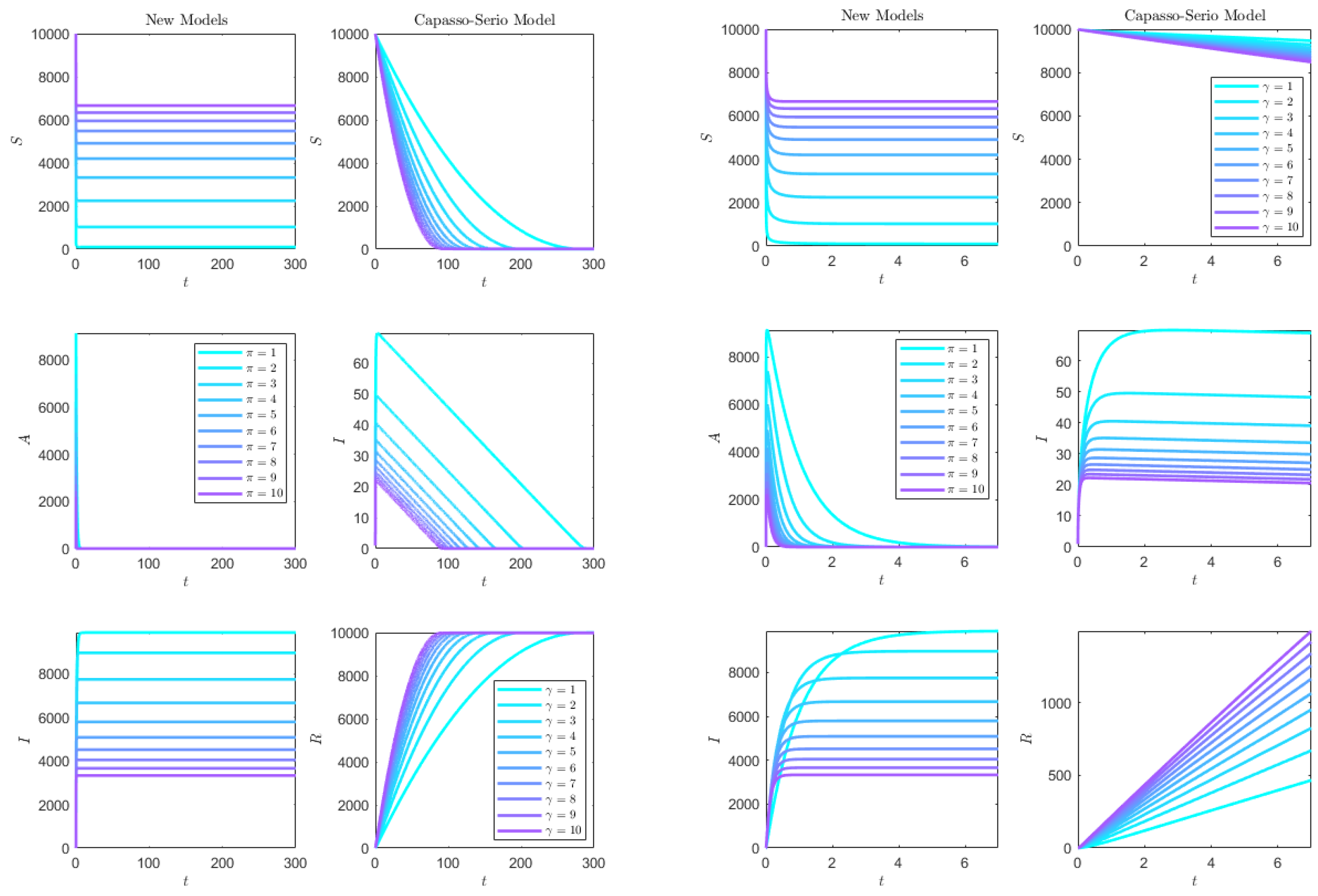
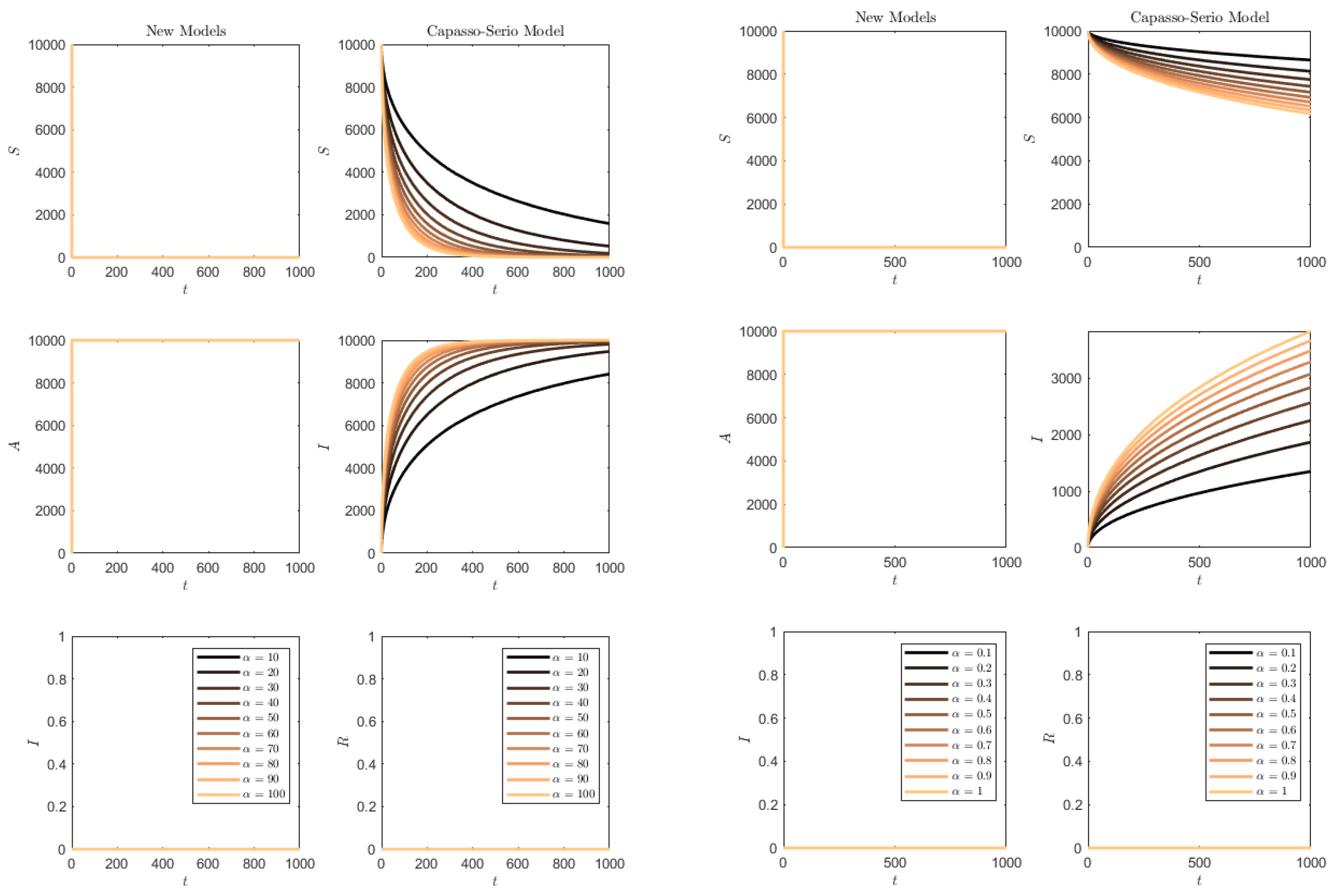
In both Figure 10 and Figure 11, while in the classical model (73) ultimately almost the whole population is affected, a good number of susceptibles are preserved in the SAI model (1). For the (73) model, the higher the removal rate $\gamma$, the faster the disease affects the population, Figure 10. Instead, for the SAI model, the higher the progression rate $\pi$, the higher the number of susceptibles that are preserved from the disease. A similar effect is noted if the disease contact rate $\alpha$ increases, Figure 11.

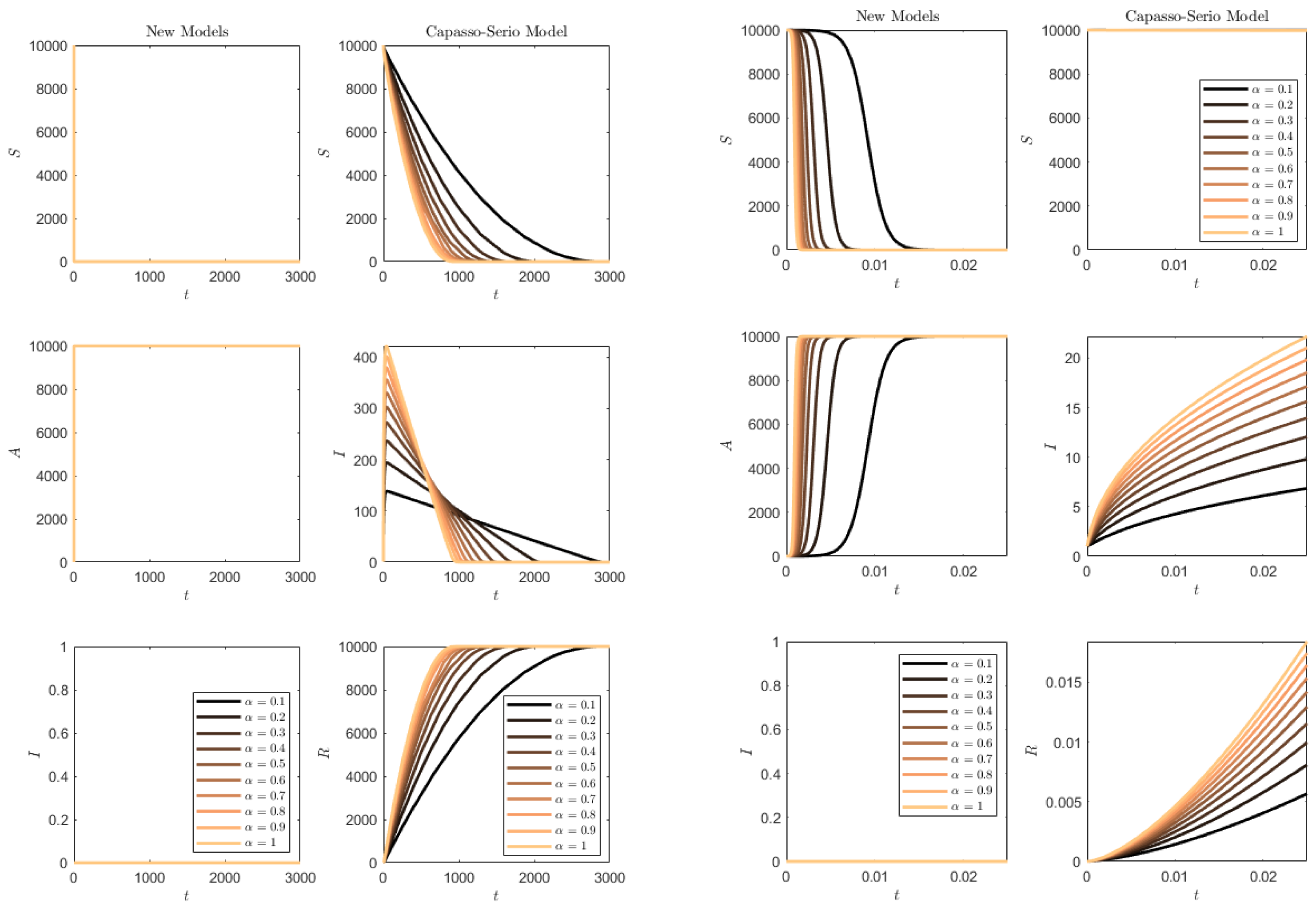
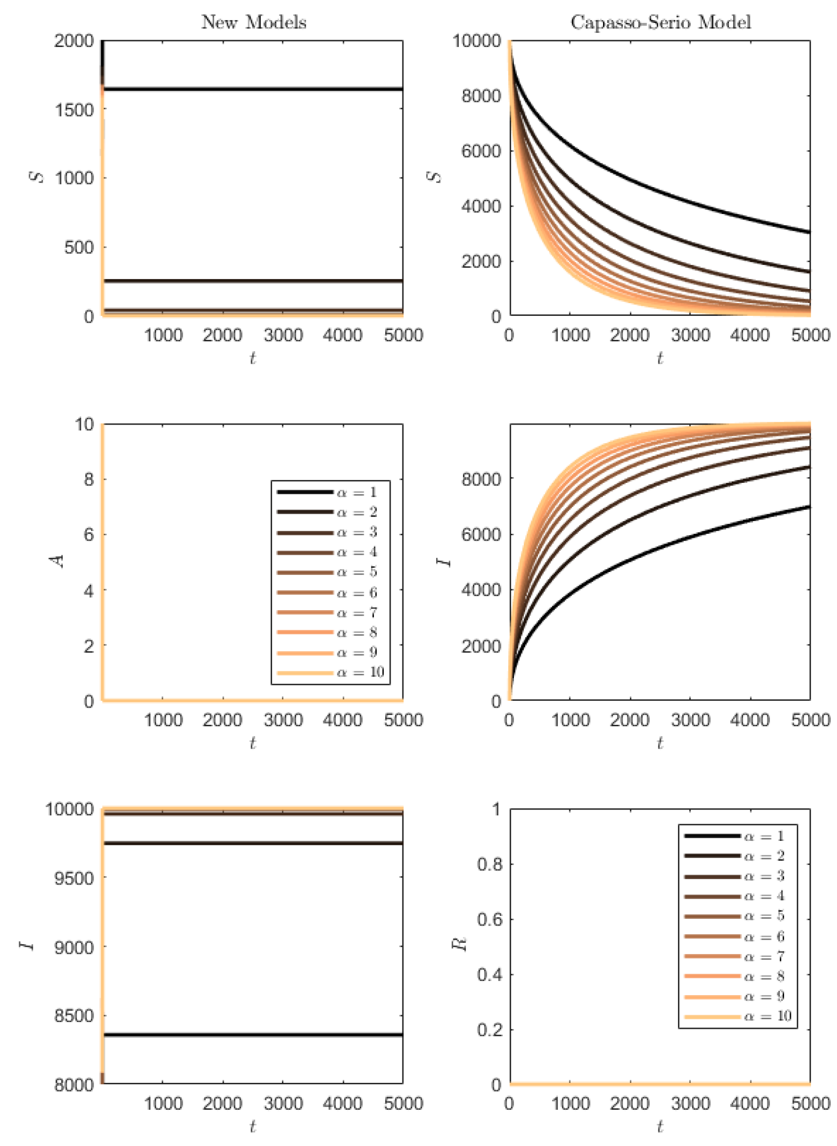
Figure 12 contains the simulation of the opposite conditions: higher transmission rate than progression/removal rates. In this situation, the susceptibles of the SAI model (1) are quickly depleted and the whole population quickly becomes symptomatic. For (73), this occurs much more slowly, and the slower the smaller the transmission rate is.

We next compare the two types of models as different versions of the SI model, with just asymptomatics in (1) and recognizable infected for (73). We, thus, take $\pi =\gamma =0$ to prevent progression respectively to symptomatics or removed. Figure 13 contains the results of the simulations in this case. In the case of model (73), the R compartment is initially empty and, in this case, clearly remains empty throughout the simulation. For the SAI model, there is no progression to symptomatics and, also, this compartment is empty. It is interesting to note that the lower values of $\alpha$ once again have a delaying effect on the epidemics’ propagation for (73), the more marked the lower the value of the rate $\alpha$. However, in the SAI model, everyone is very quickly affected and the susceptibles are quickly depleted. The important remark is that the behavior remains in agreement with the ones found in the former, Figure 12, since $\pi =0<\alpha$.

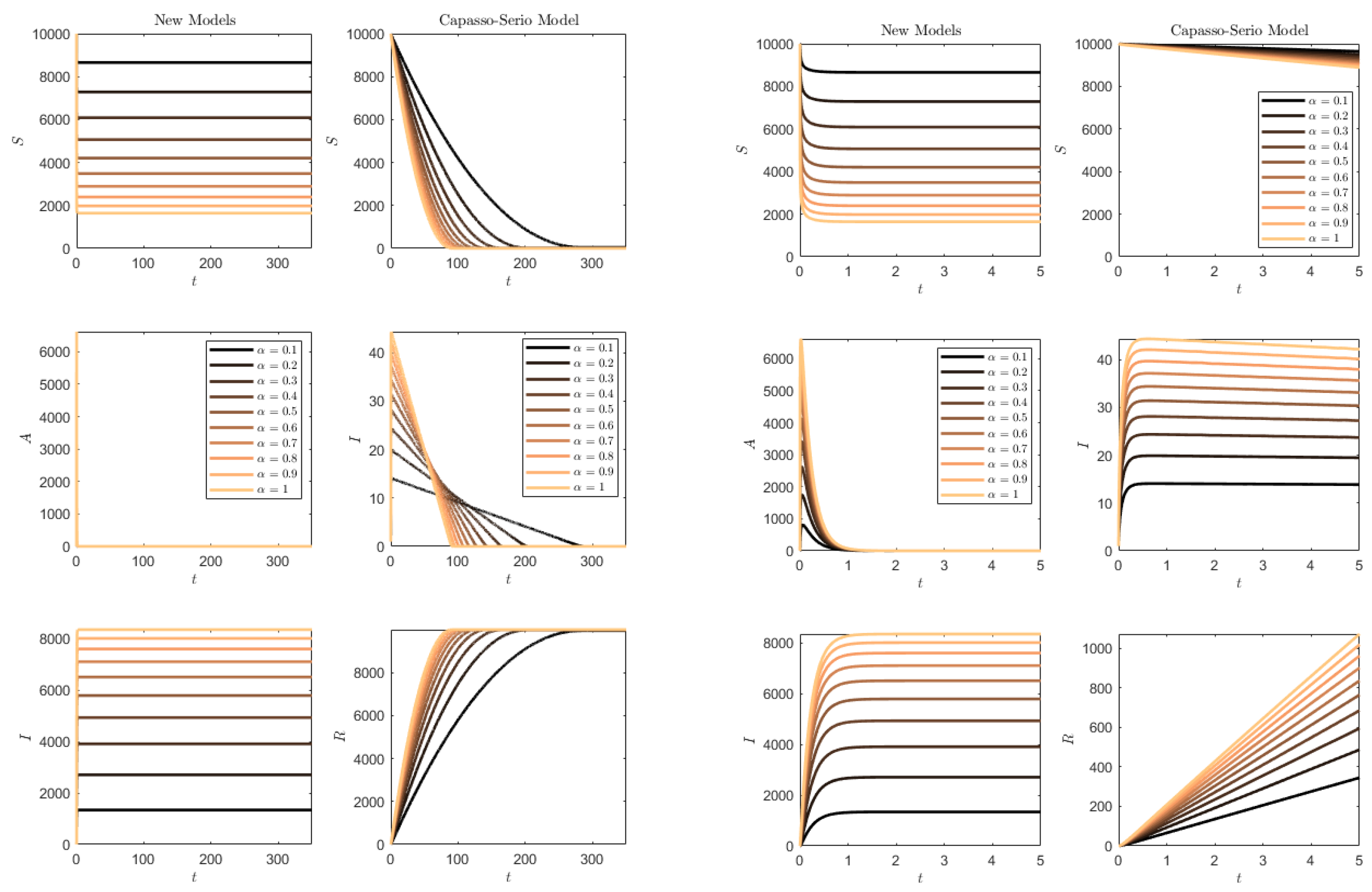
We also compared the two models (1) and (73), interpreting the former as an extension of the SI model, allowing in it two classes of individuals affected by the disease: asymptomatic and symptomatic. This is performed by allowing progression from A to I, while there is no removal rate in the classical model. Hence, $\pi \ne 0$ and $\gamma =0$. Figure 14 shows the results. It is clearly seen that for $\alpha <\pi$, the SAI model preserves again part of the susceptibles, while this does not occur for (73), and for $\alpha >\pi$ in both models the whole population is affected.

We finally consider a less relevant simulation, for the reverse case $\pi =0$ and $\gamma =0.05$. This is not a fair comparison as on one hand we have an SA model (the SI model with all asymptomatics) versus a full SIR model. In the former case, everybody becomes asymptomatic and in the latter, almost everyone also contracts the disease, within a timespan that is longer the lower the contact rate. The results are not shown, as they coincide with Figure 13.

The simulations for model (1), or equivalently (23), show a much higher impact of the disease. For increasing disease contact rate, the susceptibles are very much reduced, and symptomatic people rise to high values, Figure 11; instead, the asymptomatic ones quickly vanish. Higher progression rates from asymptomatic to symptomatic are beneficial, because they increase the number of susceptibles and sensibly reduce the symptomatic individuals.

6. Conclusions

In this paper, we analysed a simple disease transmission system with some demographic features. The illness is assumed to develop at first in an asymptomatic form. The model accounts for epidemic-induced fear in the population, for which measures are taken to reduce contacts. The main novelty is represented by the fact that susceptibles respond not to a large number of asymptomatic infected, but just to the size of the symptomatic individuals compartment.

The demographic part of the model accounts for inter- and intraspecific pressures among the various compartments, but this is not symmetric. Specifically, such pressure could be reduced in the class of symptomatic infected I, because they are known to be sick and are, therefore, supposedly being cared for. Alternatively, it could be higher, meaning that being debilitated by the disease, they feel more the competition of other compartments. They instead exert a pressure on the other classes; this could be interpreted, e.g., as a burden, namely, the costs for the society to hospitalize them. This is very approximate and could be modified and expanded, if needed.

However, our main focus lies on the epidemiology. The susceptibles become infected by the asymptomatic in a mild form, migrating, indeed, into the asymptomatic class. This could be criticized and improved, but it is essential in order to compare the results with the classical model (73). Considering other infection mechanisms that may lead directly from susceptibles to symptomatic individuals, this would indeed significantly change the model and make the comparison less fair. In this way, both in (1) as well as in (23), because in the absence of demographics they coincide, the transition between compartments is the same used in (73). Thus, the simulations’ results can be compared in an adequate way. There is only a minor mathematical change of a technical nature, in that the response function depends inversely on $1+\beta I^2$ in (73), and this is necessary to push it to zero for large values of I, while for the SAI case it is enough for it to be inversely proportional to $1+\beta I$, in view of the fact that in the numerator no I appears.

The main finding in the simulations is that the SAI model introduced here, in spite of being an SI-type model with the infected individuals split between two classes, asymptomatic and symptomatic, may prevent some susceptibles from contracting the disease, in the proper situation, in contrast to the classical SI model. Specifically, this occurs if the progression rate from asymptomatic to symptomatic is above the contact rate. The progression rate plays, thus, a fundamental role. The explanation for this situation lies in the fact that for a high progression rate, the asymptomatic class is fast depleted so that the symptomatic reaches high numbers quickly. As a consequence, the transmission rate in the SAI model quickly approaches zero, because the denominator grows and the numerator is reduced. Specifically, for the single susceptible the infected washout rate should exceed their recruitment rate i.e.,

$$\frac{\alpha I}{1+\beta I}<\pi .$$

Thus the minimum weight that the individuals should give on the information about the symptomatics, can be assessed by finding the critical threshold ${\beta }^{†}$

$${\beta }^{†}=\frac{\alpha }{\pi }-\frac{1}{I}$$

where I is the number of observed symptomatics. In this way for $\beta >{\beta }^{†}$ the ratio of transmission to progression rates falls below one, and a number of susceptibles are preserved from getting the disease, the higher the farther $\beta$ is from the critical threshold. The transmission rate of model (73), instead, contains the infected I also in the numerator. Thus, although the denominator grows quickly because it contains the term $1+\beta I^2$, the transmission rate reaches zero at a slower pace than the SAI model does. This phenomenon represents an instance of the well-known fact that diseases that severely affect individuals preserve instead the whole community, while they significantly impact the population if they are mild at the individual level.

This analysis shows that the determination of whether a disease is asymptomatic and the assessment of the progression and transmission rates proves fundamental for its possible containment. In addition, in the presence of asymptomatic diseased individuals, the individual protection measures should have a higher impact, measured by a larger weight coefficient $\beta$, when just a few symptomatics appear in the population. The simulations of Figure 10 and Figure 11 also help in quantifying the disease impact on the population, if a reliable measure of the contact rate $\alpha$, as well as of the transition rate to symptomatic $\pi$, exist.

Overall, this investigation reveals the importance of properly assessing these rates as soon as possible. It also stresses that accounting for asymptomatics in the individual response as well as in the epidemic control is of utmost importance.