An Analytical Solution to the One-Dimensional Unsteady Temperature Field near the Newtonian Cooling Boundary

Abstract

One-dimensional heat-conduction models in a semi-infinite domain, although forced convection obeys Newton’s law of cooling, are challenging to solve using standard integral transformation methods when the boundary condition φ(t) is an exponential decay function. In this study, a general theoretical solution was established using Fourier transform, but φ(t) was not directly present in the transformation processes, and φ(t) was substituted into the general theoretical solution to obtain the corresponding analytical solution. Additionally, the specific solutions and corresponding mathematical meanings were discussed. Moreover, numerical verification and sensitivity analysis were applied to the proposed model. The results showed that T(x,t) was directly proportional to the thermal diffusivity (a) and was inversely proportional to calculation distance (x) and the coefficient of cooling ratio (λ). The analytical solution was more sensitive to the thermal diffusivity than other factors, and the highest relative error between numerical and analytical solutions was roughly 4% under the condition of 2a and λ. Furthermore, T(x,t) grew nonlinearly as the material’s thermal diffusivity or cooling ratio coefficient changed. Finally, the analytical solution was applied for parameter calculation and verification in a case study, providing the reference basis for numerical calculation under specific complex boundaries, especially for the study of related problems in the fields of fluid dynamics and peridynamics with the heat-conduction equation.

1. Introduction

In practical engineering and physical problems, the physical quantity to be analyzed is affected by more than one variable; thus, it is generally expressed in partial differential equations. For the needs of practice and application, Fourier elucidated the phenomenon of heat conduction and presented a series of laws related to heat conduction, i.e., the classical heat conduction equations in 1822; his research greatly impacted the development of partial differential equations [1]. Heat conduction appears in many mathematical models. The difference equation in the famous Black Scholes model can be transformed into heat conduction and a simple solution can be derived, but many extension models have no analytical solution. Thus, numerical methods are used for the calculation. For example, the Crank–Nicolson method can be used to effectively determine the numerical solution of heat conduction, and this method can also be used in many models without an analytical solution [2]. Fayz et al. expressed a numerical study of flow features and heat transport inside an enclosure. Governing equations were discretized by a finite-element process with a collected variable arrangement. Streamlines and isotherm lines were utilized to show the corresponding flow and thermal field inside a cavity. Velocity and temperature profiles were displayed for some selected positions inside an enclosure for a better perception of the flow and thermal field [3]. Moreover, Navier–Stokes equations are motion equations that describe the momentum conservation of viscous incompressible fluids. They reflect the basic mechanical laws of viscous fluid flow and are of great significance in fluid mechanics, but they are nonlinear partial differential equations, which are very difficult and complex to solve. Moreover, they can be simplified to obtain an approximate solution in some cases. Since the rapid development of computers, the numerical solution of Navier–Stokes equations have made great progress. However, in terms of analytical solutions, the exact solutions can only be obtained on some very simple special flow problems, and further development and novel ideas or technologies are required to obtain the analytical solutions.

Therefore, the heat-conduction equation is an important development equation in partial differential equations and an important theoretical equation in the fields of fluid mechanics [4], materials [5], and bioengineering [6]. In the classical one-dimensional heat-conduction model [7,8], the boundary temperature φ(t) is a known constant ∆T₀ (i.e., the boundary temperature increases ∆T₀ at the initial instantaneous change and then remains unchanged) when the temperature field follows the first boundary control condition. Here, the analytical solution of the model can be directly obtained using integral transformation methods, such as Laplace transform or Fourier transform [8,9,10]. Through Newton’s law of cooling and Fourier’s law, combined with the relevant physical parameters, Tan et al. established the heat-conduction model of the fire suit and the model could improve the fitting accuracy, which is of great significance for the design and of and research into specialist fire clothing and equipment, and also had a certain reference value for solving similar problems [11]. It could also be directly solved using integral transformation when the boundary condition had a relatively simple function form, such as a time linear function [9,12,13,14]. However, it is difficult to solve when φ(t) is a definite function form due to its complexity, and the solution can be expressed or an approximate solution can be obtained [15,16] by using the special functions [17,18].

The heat-conduction model has always been an important research component of mathematical and physical methods [7,8,9]. For instance, Dominic et al. [17] studied the analytical solution to the unsteady one-dimensional conduction problem with two time-varying boundary conditions, Weigand et al. [19] studied the analytical methods for heat transfer and fluid flow problems, and Burggraf et al. [20] studied an exact solution of the inverse problem in heat conduction. Nevertheless, in practical engineering applications, some common problems still exist. According to Newton’s law of cooling [21], objects transfer heat to the surrounding medium when their temperature is higher than that of the environment, which is one of the fundamental laws of heat transfer. For example, in the ground source heat-pump system, the circulating water temperature in the heat exchanger is naturally cooled, and the geothermal heat conduction around the heat exchanger can be regarded as a heat conduction problem under the boundary conditions of Newton’s law of cooling. To prevent the impact of high temperature on the performance and safety of a power battery, Ma Yan et al. applied Newton’s cooling law, established the battery resistance of the battery with temperature change, determined the convection heat transfer coefficient changes with the coolant flow rate of the cell concentrated-mass heat model, and proposed a fuzzy proportional-integral-derivative direct liquid-cooling strategy for a battery pack [22]. Rosales et al. used a generalized conformable differential operator and then a simulation of the well-known Newton’s law of cooling was made, which had an advantage with respect to ordinary derivatives [23]. Melo et al. developed an active thermography algorithm capable of detecting defects in materials, based on the techniques of thermographic signal reconstruction, thermal contrast, and the physical principles of heat transfer. Newton’s law of cooling was used to store the normalized temperature data pixel-by-pixel over time and a compression ratio of 99% was obtained [24]. Konovalenko et al. proposed a novel method that extends the applicability of Newton’s law of cooling to changeable ambient temperatures based on a set of temperature stability conditions and a sensor measurement error. In this method, an optimal number of measurements that characterize stable ambient temperatures and improve prediction reliability are selected [25]. Calvo-Schwarzwlder et al. simulated the growth of a one-dimensional solid by considering a modified Fourier law with a size-dependent effective thermal conductivity and a Newton cooling condition at the interface between the solid and the cold environment [26]. Herrera-Sánchez et al. used Newton’s Law of Cooling for heat transfer, which states the rate of heat exchange between an object and its environment, to solve the problem of the packaging process when handling canned food [27].

In practice, even if the immediate increase in the boundary temperature and subsequent decline are consistent with Newton’s law of cooling, the heat transfer issue is challenging to solve directly by integral transformation when the boundary conditions are the exponential decay function ∆T₀ e^−λt. Moreover, for the above one-dimensional heat-conduction model, from the perspective of mathematical physical models, many problems in nature have similar physical laws, such as diffusion, cooling, charge and discharge, particle spin polarization degree, and other system state evolutions over time. Moreover, the solving of partial differential equations is equivalent to calculating a particular solution under a specific boundary condition [28,29,30,31,32,33,34,35,36,37,38,39,40,41,42,43,44,45,46]. The physical law for describing the temporal temperature decrease has been dominated by Newton’s law of cooling (NLC), which assumes that natural cooling occurs by following an exact exponential trend. However, several studies have questioned the broad validity of this law by arguing that cooling occurs following an approximate rather than an exact exponential trend. Silva introduced a new formulation of NLC based on generalized statistics that outperforms the classical NLC, and so demonstrates a new path to cooling analyses [47]. Yan et al. studied a discrete variable topology optimization method to solve the simplified convective heat transfer (SCHT) design optimization modeled by Newton’s law of cooling. The discrete variable topology optimization was based on the proposed sequential approximate integer programming with trust-region, which could identify the convective boundary and carry out the optimization design [48]. Thus, the heat-conduction model with the boundary conditions of Newton’s law of cooling needs to be studied.

The goal of this work was to analyze the mathematical and physical implications of a one-dimensional heat-conduction model in a domain with a semi-infinite border using Newton’s law of cooling as a boundary condition. More significantly, the analytical solution approaches that are suggested were examined from the standpoint of fusing mathematical significance with real-world application requirements. For specific research content, the operator of φ(t) was used in the model transformation and inverse transformation processes to establish a general theoretical solution. Furthermore, the boundary condition function does not directly participate in the transformation based on the inverse Fourier transformation and the differential properties of the convolution method [8,9]. Then, φ(t) = ∆T₀ e^−λt was substituted into the general theoretical solution, and the analytical solution of this problem is obtained. Note that although the formal transformation of φ(t) was not performed, the boundary function must meet the Fourier transformation requirements. Additionally, the specific solutions and corresponding mathematical meanings are discussed. Numerical verification and sensitivity analysis are performed for the proposed model. Finally, an analytical solution is applied for parameter calculation and verification in the case study. The proposed solution method is relatively simple and convenient and does not have the complicated transformation and inverse transformation operation processes of φ(t).

The proposed method aims to guide the actual process of solving the reverse heat conduction reverse problem. This could provide a reference basis for numerical calculation under specific complex boundaries, especially for similar physical laws. Finally, the measurement point arrangement and measurement effect inspection of heat sensitive sensors depend on the distribution characteristics of the temperature field in the detection parts. Thus, the analytical solution of the temperature field under the influence of different temperature boundary conditions will provide a convenient and reliable theoretical method for analyzing the temperature field distribution characteristics in different detection parts.

2. Basic Model and Its Solution

In engineering practice, most heat exchange holes are arranged in a dense line in ground coupling heat-pump system, and the heat exchange holes are regarded as a single hole. The water temperature of the linearly arranged heat exchange hole is generalized as the first temperature boundary (Dirichlet boundary). Here, the geothermal field change of the heat-pump system can be generalized into a one-dimensional heat conduction problem in the semi-infinite domain.

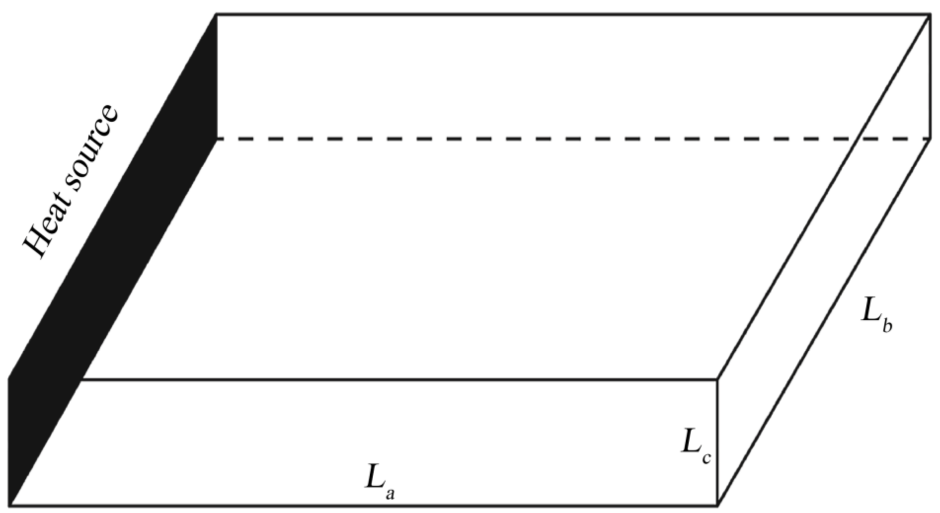
Based on the above a thin-layer material with a heat source at one boundary was taken as an example, as shown in Figure 1. The heat transfer characteristics of materials can be summarized as follows: (1) The experimental material is homogeneous and isotropic and extends infinitely in the x-direction. (2) One boundary of the material is provided with a heat source under the Dirichlet boundary condition, whereas the outer surface of the other boundary is a heat insulation surface. (3) The initial temperature of the material and boundary is T(x,0) = 0, and the temperature field is recorded as T(x,t). (4) The time variation function of the boundary temperature is denoted as φ(t). (5) The heat transfer in the thin layer material is one-dimensional heat conduction, and the temperature field near the boundary is shown in Figure 2.

The above heat conduction problem can be depicted as a mathematical model (I) [49]:

$$(\mathrm{I})\left\{\begin{array}{lll}\frac{\partial T}{\partial t}=a\frac{{\partial }^{2}T}{\partial x^2}\hfill & (0<x<+\infty ,t>0)\hfill & (1)\hfill \\ T(x,t)\left|{}_{t=0}\right.=T(x,0)\hfill & (x>0)\hfill & (2)\hfill \\ T(x,t)\left|{}_{x=0}\right.=T(0,0)+\phi (t)\hfill & (t>0)\hfill & (3)\hfill \\ T(x,t)\left|{}_{x\to \infty }\right.=T(x,0)\hfill & (t>0)\hfill & (4)\hfill \end{array}\right.$$

where t (s) is the time, x (m) is the distance from the calculation point to the boundary, a (m²/s) is the thermal diffusivity or thermal conductivity of the solid material, T(x,t) (°C) is the temperature, and φ(t) is a boundary function.

Model (I) is the basic model. In porous media seepage mechanics, T(x,t) is generally denoted as H(x,t) to represent the water level and a (m²/d) is the permeability coefficient of the porous media [12,13,14]. In environmental hydraulics, T(x,t) is generally denoted as C(x,t) to represent the water quality concentration, wherein parameter a is mostly written as D (m²/d), which is the hydrodynamic diffusion coefficient [50].

In model (I), the boundary condition (3) is x = 0: T(x,t) = T(0,0) + φ(t). So that the converted model does not rely on the initial time value of the model, the following Fourier transform is applied. Set u(x,t) = T(x,t) − T(x,0), and then, in model (II), the boundary condition (7) is converted to u(x,t) = φ(x,0). Model (II) is as follows [7]:

$$(\mathrm{II})\left\{\begin{array}{lll}\frac{\partial u}{\partial t}=a\frac{{\partial }^{2}u}{\partial x^2}\hfill & (0<x<+\infty ,t>0)\hfill & (5)\\ u(x,t)\left|{}_{t=0}\right.=0\hfill & (x>0)\hfill & (6)\\ u(x,t)\left|{}_{x=0}\right.=\phi (t)\hfill & (t>0)\hfill & (7)\\ u(x,t)\left|{}_{x\to \infty }\right.=0\hfill & (t>0)\hfill & (8)\end{array}\right.$$

where u(x,t) is the temperature relative to the initial temperature field.

When a definite function of φ(t) exists such that ∆T₀ is constant in the classical model, model (II) can be solved via Fourier transform and Laplace transform.

For the above problem, in particular, the PDE is linear and a simple mathematical model. There is a very hot field in mathematics and physics that has been studying nonlinear PDE for a long time. For example, Md and Cemil examined the modified (G′/G)-expansion process for generating closed-form wave answers of the conformable fractional ZK equation, including power law nonlinearity [51]. So, in the future research, the related nonlinear PDE equations could be studied further.

3. General Theoretical Solution

The heat conduction equation can be solved using methods such as analytical, approximate analytical, and numerical methods. Numerical methods are usually used to deal with this kind of heat conduction problem. Calculation tools and analysis techniques are fairly advanced, and numerical methods have become the main means for solving the complex heat conduction problems [52]. However, strict analytical solutions can only be obtained under certain specific conditions. In most cases, especially under transient conditions, the strict solution is either too cumbersome or does not exist at all. In existing research, the heat-conduction model and its analytical solution for a ground source heat-pump system are given, and the heat conduction outside a borehole can be generalized as an infinite or a finite length linear heat source releasing heat to the surrounding soil [53,54]. The problem can also be regarded as an unsteady heat-conduction process from the column heat source to the surrounding infinite area [55]. A Kelvin line or infinite line heat source analytical model is established based on Fourier heat conduction law. The theory usually assumes that a borehole is an infinite linear heat source, and the Earth is an infinite homogeneous medium with a specific initial temperature [53,56,57]. Moreover, the column heat source model is based on the Fourier heat conduction law. Assuming that the heat transfer rate is a constant value, Carslaw and Jaeger established the transient heat conduction control equation under the given boundary conditions and initial conditions [7]. Eskilson assumed that a borehole is a limited linear heat source and considered the heat flux along the borehole axis; thus, their model is suitable for the long-term operation of the ground source heat-pump system [58]. Based on the Eskilson theory, Zeng et al. considered the influence of finite borehole length with the surface as the boundary, and they derived the analytical solution of a transient finite-line heat source mode [54]. To solve complex mathematical problems, analytical models usually have some restrictive assumptions and simplifications, and the accuracy of analytical results is reduced [59]. However, analytical models have high calculation efficiency and require low calculation times.

According to the above research, using Fourier transform to solve the analytical solution in the heat-conduction mode is feasible. In terms of the properties of the transformation of φ(t), the general theoretical solution of this kind of model is given separately. The process does not depend on the transformation of φ(t).

For model (II), the variation range of x is 0–+∞. Thus, the Fourier sinusoidal transformation of x can be solved. According to the characteristics and properties of Fourier transform, the following calculation process is obtained [60]:

$$F[u(x,t)]={\displaystyle {\int }_0^{\infty }u(x,t)\sin \omega xdx=}\overline{u}(\omega ,t)$$

(9)

$$F\left[\frac{\partial u}{\partial t}\right]=\frac{d\overline{u}}{dt}$$

(10)

$$F\left[\frac{{\partial }^{2}u}{\partial x^2}\right]={\displaystyle {\int }_0^{\infty }\frac{{\partial }^{2}u}{\partial x^2}\sin \omega xdx=}{\left.\omega u\right|}_{x=0}-{\omega }^2\overline{u}$$

(11)

where $\overline{u}$ is the Fourier transform of u for x, ω is the Fourier transform operator, and F is the transform operator.

From Equation (5) with the boundary condition (7), the results are as follows:

$$\frac{d\overline{u}}{dt}=a[\omega {\left.u\right|}_{x=0}-{\omega }^2\overline{u}]=a[\omega \phi (t)-{\omega }^2\overline{u}]$$

(12)

The upper equation is a first-order inhomogeneous linear differential equation, and its general solution is

$$\overline{u}(\omega ,t)=e^{-{\omega }^{2}at}\left[{\displaystyle {\int }_0^{t}a\omega }{\left.u\right|}_{x=0}{e}^{{\omega }^{2}a\xi }d\xi +C\right]$$

(13)

where C is the pending constant.

When solving the special solution of the model (II), the pending constant C must first be determined according to the fixed solution condition Equation (6). Thus, when u(x,t) = 0, $\overline{u}(\omega ,t)$ = 0.

$$C=-\left({\displaystyle {\int }_0^{t}a\omega }{\left.u\right|}_{x=0}{e}^{{\omega }^{2}a\xi }d\xi \right)\left|{}_{t=0}\right.=0$$

(14)

After the pending constant C is determined, then by Equations (13) and (14),

$$\overline{u}(\omega ,t)=e^{-{\omega }^{2}at}{\displaystyle {\int }_0^{t}a\omega }{\left.u\right|}_{x=0}{e}^{{\omega }^{2}a\xi }d\xi$$

(15)

Substitute the boundary condition Equation (7) of the model (II) into Equation (14), and the particular solution of the model (II) is

$$\overline{u}(\omega ,t)=e^{-{\omega }^{2}at}{\displaystyle {\int }_0^{t}a\omega }\phi (\xi )e^{{\omega }^{2}a\xi }d\xi$$

(16)

For Equation (16), the inverse sine transform is obtained; then,

$$\begin{array}{cc}\hfill u(x,t)& =F^{-1}\left[\overline{u}(\omega ,t)\right]=\frac{2}{\pi }{\int }_0^{\infty }\overline{u}(\omega ,t)sin\omega xd\omega =\frac{2}{\pi }{\int }_0^{\infty }\left[e^{-{\omega }^{2}at}{\int }_0^{t}a\omega \phi \left(\xi \right)e^{{\omega }^{2}a\xi }d\xi \right]sin\omega xd\omega \hfill \\ & =\frac{2a}{\pi }{\int }_0^t\phi \left(\xi \right)\left[{\int }_0^{\infty }\omega e^{-{\omega }^{2}a(t-\xi )}sin\omega xd\omega \right]d\xi \hfill \\ & =\frac{2a}{\pi }{\int }_0^t\phi \left(\xi \right)\left\{{\left[\frac{1}{-2a(t-\xi )}{e}^{-{\omega }^{2}a(t-\xi )}\right]}_0^{\infty }+\frac{1}{2a(t-\xi )}{\int }_0^{\infty }{e}^{-{\omega }^{2}a(t-\xi )}xcos\omega xd\omega \right\}d\xi \hfill \\ & =\frac{x}{\pi }{\int }_0^t\frac{\phi \left(\xi \right)}{t-\xi }\left[{\int }_0^{\infty }{e}^{-{\omega }^{2}a(t-\xi )}cos\omega xd\omega \right]d\xi \hfill \end{array}$$

(17)

where F⁻¹ is the inverse conversion operator.

To solve the above equation, the relation between inverse sine and cosine transform is applied, and the order of integral exchange is focused on.

According to the known integral Equation (18) [60],

$${\displaystyle {\int }_0^{\infty }{e}^{-b{\omega }^2}}cos\omega xd\omega =\left[\sqrt{\pi }/\left(2\sqrt{b}\right)\right]e^{-x^2/4b}$$

(18)

where b is the intermediate variable, b = a (t − ξ).

Combining with Equation (17), u(x,t) can be written as

$$u(x,t)=\frac{x}{2\sqrt{\pi a}}{\displaystyle {\int }_0^t\left[\frac{\phi (\xi )}{{(t-\xi )}^{3/2}}\exp \left(-\frac{x^2}{4a(t-\xi )}\right)\right]}d\xi$$

(19)

where ξ is the integral variable in time.

Equation (19) is the solution of a one-dimensional heat-conduction model in semi-infinite domain when the boundary condition is φ(t).

φ(t) is not directly engaged in the transformation throughout the calculating procedure. Thus, a solution method for the model is provided when φ(t) is complex and difficult to directly solve using Fourier transform.

According to the definition of convolution and the properties of Fourier transform, the commonly used solution can be obtained in the form of the probability density function. Thus, Equation (19) can be written as

$$u(x,t)=\phi (\xi )\ast \left[\frac{x}{2t\sqrt{\pi at}}\exp \left(-\frac{x^2}{4at}\right)\right]=\phi (\xi )\ast \frac{d}{dt}\left[\frac{2}{\sqrt{\pi }}{\displaystyle {\int }_{\frac{x}{2\sqrt{at}}}^{+\infty }{e}^{-{\tau }^2}d\tau }\right]=\phi (\xi )\ast \frac{d}{dt}\left[erfc\left(\frac{x}{2\sqrt{at}}\right)\right]$$

(20)

where the asterisk is the convolution operator in Equation (19).

According to the differential properties of convolution

$$\phi (t)\ast \frac{d}{dt}\left[erfc\left(\frac{x}{2\sqrt{at}}\right)\right]+{\left.erfc\left(\frac{x}{2\sqrt{at}}\right)\right|}_{t=0}\cdot \phi (t)=erfc\left(\frac{x}{2\sqrt{at}}\right)\ast \frac{d\left[\phi (t)\right]}{dt}+{\left.\phi (t)\right|}_{t=0}\cdot erfc\left(\frac{x}{2\sqrt{at}}\right)$$

(21)

Note the equivalence between the third line of Equation (20) and the first item at the left side of Equation (21). When ${\left.erfc\left[x/\left(2\sqrt{at}\right)\right]\right|}_{t=0}=0$, Equation (21) can be rearranged as follows:

$$u(x,t)=\phi (t)\ast \frac{d}{dt}\left[erfc\left(\frac{x}{2\sqrt{at}}\right)\right]={\left.\phi (t)\right|}_{t=0}\cdot erfc\left(\frac{x}{2\sqrt{at}}\right)+erfc\left(\frac{x}{2\sqrt{at}}\right)\ast \frac{d[\phi (t)]}{dt}$$

(22)

Using the commutative law of convolution, the above formula can be written in integral form as

$$T(x,t)=T(x,0){\left.+\phi (t)\right|}_{t=0}\cdot erfc\left(\frac{x}{2\sqrt{at}}\right)+{\displaystyle {\int }_0^t\frac{d[\phi (\zeta )]}{d\zeta }\cdot erfc\left(\frac{x}{2\sqrt{a(t-\zeta )}}\right)}d\zeta$$

(23)

Equation (23) is the model solution obtained without direct transformation of the boundary condition φ(t), that is, the solution is valid for all boundary conditions of φ(t). Therefore, Equation (23) is the general theoretical solution of this kind of model. When the function form of φ(t) is determined, the solution can be obtained by substituting φ(t) into Equation (23).

In the transformation process, φ(t) is operated in the form of the operator; thus, it should meet the requirements of Fourier transform. Moreover, φ(t) is integrable on any interval under the Dirichlet condition [50]. Additionally, it meets the above requirements when φ(t) is the exponential decay function.

For a one-dimensional heat-conduction model under the first boundary condition of homogeneous medium in a semi-infinite domain, the general theoretical solution was obtained under the complex form of the boundary condition function. Furthermore, the process applied to the general theoretical solution can provide a reference for solving similar problems in other fields, such as the contamination migration problem under the natural decay boundary conditions of source concentration in the subsoil.

4. Solutions to the Newton’s Law of Cooling Boundary

To investigate the analytical solution of a one-dimensional unsteady temperature field near the Newton’s law cooling boundary, the general theoretical solution of this kind of model is given based on Fourier transform. The integration transformation and the inverse transformation processes do not depend on the expression or function form of φ(t) = ∆T₀ e^−λt, where λ is the coefficient of cooling ratio, and the corresponding physical significance of λ is an indicator of the speed of temperature change under the Newton’s law of cooling boundary.

The general solution gives the form of the solution, including all solutions that satisfy the differential equation. When the initial conditions of the differential equation are given, specific values of the parameter can be determined and a unique special solution can be obtained. According to the actual situation, the special solutions under three kinds of boundary conditions are as follows: (1) λ > 0, Newton’s law of cooling boundary condition, that is, the solution of the nonlinear variation problem. (2) λ = 0, the boundary temperature remains unchanged after instantaneous change. (3) The boundary temperature changes linearly after the instantaneous change.

4.1. The Newton’s Law of Cooling Boundary

When λ > 0, after the boundary temperature instantaneously increases by ∆T₀ and then cools naturally according to Newton’s law of cooling, the boundary temperature is φ(t) = ∆T₀e^−λt, which is substituted into Equation (23):

$$T(x,t)=T(x,0)+\mathsf{\Delta }{T}_0\cdot erfc\left(\frac{x}{2\sqrt{at}}\right)-\lambda \cdot \mathsf{\Delta }{T}_0{\displaystyle {\int }_0^t{e}^{-\lambda \zeta }\cdot erfc\left[\frac{x}{2\sqrt{a(t-\zeta })}\right]}d\zeta$$

(24)

By simply replacing the boundary conditions into the general theoretical solution, the model solution is produced under the Newtonian cooling boundary. This solution procedure can be used for models whose boundary conditions are other forms of function, circumventing the complicated transformation process.

4.2. The Fixed Boundary Condition

When λ = 0, for the convenience of discussion, e^−λt is expanded using a power exponential form:

$$e^{-\lambda t}=1+{\displaystyle \sum _{n=1}^{\infty }\frac{{(-\lambda t)}^n}{n!}}$$

(25)

φ(t) = ∆T₀ under the condition of λ = 0. The corresponding physical meaning is that when the boundary temperature remains unchanged after the instantaneous change of ∆T₀, this is the general boundary condition in the classical model.

Here, the second term on the right side of Equation (25) is zero, and Equation (24) is transformed into the solution of the classical model, that is, the solution of the classical problem is a special case of Equation (23).

4.3. The Linear Boundary Condition

When λ ≠ 0∩φ(t) = ∆T₀(1 − λt), the boundary temperature changes linearly after the instantaneous change. Equation (25) is an alternating series term, for example, the first two terms of the series are taken in the process. φ(t) = ∆T₀(1 − λt), which means that after the temperature instantaneously increases by ∆T₀, the boundary temperature starts to slowly decrease with a slope of λ∆T₀. Then, from Equation (24),

$$T(x,t)=\mathsf{\Delta }{T}_0\left[erfc\left(\frac{x}{2\sqrt{at}}\right)-\lambda {\displaystyle {\int }_0^{t}erfc\left(\frac{x}{2\sqrt{a\zeta }}\right)}d\zeta \right]$$

(26)

At this time, the temperature at the boundary linearly decrease with time, and the speed of temperature change can be calculated using Equation (26). Then, the analytical solution of the model can be obtained. The boundary condition solution is relatively simple and is not described.

5. Discussion

5.1. Numerical Verification

To confirm the viability of the suggested analytical approach, parameter response regularity was examined using analytical and numerical methods. Additionally, the suggested approach was used to study the response law of the model parameters. Because of the absence of experimental data, a numerical solution was employed for comparison with the analytical solution. The explicit scheme was used for the numerical solution of Equation (1) [49] and it can be used for linear as well as nonlinear equations. The analytical and numerical solutions could be used to validate each other, and the numerical solution of the nonlinear Equation (1) can be used to show the effectiveness of the proposed method.

To derive the finite difference scheme for the nonlinear problem, the form of the explicit scheme is as follows [49]:

$$T_n^{i+1}=\frac{a\mathsf{\Delta }t}{\mathsf{\Delta }{x}^2}\left(T_{n+1}^i+T_{n-1}^i\right)+\left(1-2\frac{a\mathsf{\Delta }t}{\mathsf{\Delta }{x}^2}\right)T_n^i$$

(27)

where Δt is the time step, Δx is the space step length, (n,i) represents the position of a node in the time-space region and the corresponding temperature, recorded as T_nⁱ, T_nⁱ⁺¹ represents the temperature value of the point at x = n at time i + 1; T_nⁱ, T_n+1ⁱ and T_n−1ⁱ represent the temperature values at times i, x = n, x = n + 1 and x = n − 1, respectively.

Equation (27) constitutes the explicit computational scheme for the nonlinear Equation (1), which by mathematical experimentation is found to be stable if

$$F{o}_{\mathsf{\Delta }}=\frac{a\mathsf{\Delta }t}{\mathsf{\Delta }{x}^2}\le \frac{1}{2}$$

(28)

where Fo_Δ is the grid Fourier number.

To elucidate the analytical result, hypothetically generated data were taken and demonstrated with the help of graphs. Some hypothetical parameters were used to demonstrate the temperature behavior. Common parameters, a = 6 × 10⁻⁷ (m²/s) and λ = 0.1 (h⁻¹), were used for uniform and varying source temperature. The length of the material domain was taken as 0 ≤ x (m) ≤ 3. Figure 3a,b and Figure 4a,b were drawn for varying input parameters.

The solid curves in Figure 3a,b represent the analytical solution results for various thermal diffusivity values, 0.2a, 0.5a, a, 1.5a, and 2a, with constant λ, and the dotted curve depicts the numerical solution. The figures show that the temperature was higher for higher thermal diffusivity values. The difference value of temperature was positively related to the thermal diffusivity a, and the calculation error caused by the difference formula increased with the increase of a. The solid curves in Figure 4a,b represent the analytical solution results for various cooling ratio coefficients, 0.2λ, 0.5λ, λ, 1.5λ, and 2λ, with constant a, and the dotted curve represents the numerical solution. The figure shows that the temperature value was higher for lower cooling ratio coefficients.

In Figure 3a and Figure 4a, the comparison of temperature results is at particular time, t = 11 h. At a particular position, the temperature profile for a fixed cooling ratio coefficient increased with the thermal diffusivity. The influence of thermal diffusivity plays a significant role on temperature profile in the domain, and the influence range increased with the thermal diffusivity in Figure 3a. The cooling ratio coefficient plays a significant role in the temperature profile under the Newton’s law of cooling boundary, and the temperature variation range was between about 20 °C and 33 °C. The case results show that the boundary temperature clearly influenced the formation of the influence range in the calculation domain. Comparison of Figure 3a and Figure 4a shows that the influence range of the temperature boundary increased with a but was not affected by λ. Therefore, the temperature field study controlled by the Newtonian cooling boundary can provide a basis for the layout range and layout density of temperature sensors in space.

In Figure 3b and Figure 4b, the temperature profiles at various times are illustrated for x = 0.2 m. The figure shows that temperature was higher for lower cooling ratio coefficients. In the presence of a temperature source, the temperature in the region increased to the maximum value and then decreased with increasing time at a particular position. Comparison of Figure 3b and Figure 4b shows that the time required for the temperature to achieve stability at any spatial point in the study area decreased with increasing λ, i.e., the larger the λ, the shorter the time required for achieving stability, but it was not affected by a. Thus, the test frequency of a temperature sensor can be appropriately decreased after the temperature becomes stable. Therefore, the temperature field study controlled by the Newtonian cooling boundary can provide a basis for designing the monitoring period and frequency of the temperature sensor.

Additionally, Figure 4a clearly shows that the temperature was higher for lower λ on the boundary. In Figure 4b, in the presence of a temperature source, the temperature level initially increased but then decreases with time. On the other hand, the temperature trends had a peak inflection point, and the main contribution stems from λ.

T(x,t) is directly proportional to a and inversely proportional to x and λ, according to the calculation findings from Figure 3 and Figure 4. The highest relative error under the conditions of 2a and λ was around 4%, as determined by the relative error between the numerical and analytical solutions. This demonstrates that, compared with other factors, the analytical solution is more sensitive to thermal diffusivity. Additionally, T(x,t) grew nonlinearly if the material’s thermal diffusivity rose or the cooling ratio coefficient fell.

5.2. Sensitivity Analysis

Sensitivity analysis research varies from field to field. It is a tool for evaluating the influence of input parameters on the model output. As a result, it not only aids in the construction and validation of models but also lessens uncertainty. This study adopted the improved Morris screening method [61] and sensitivity was expressed by a dimensionless index, which was calculated as the ratio of the relative change of the model output to that of the parameters. Another approach to defining parameter changes was taken into consideration in order to increase the sensitivity of the discrimination parameters. In this approach, the change in the parameters was defined as a fixed percentage of the effective parameter range rather than a fixed percentage of the initial value [62,63].

The sensitivity discriminant factor is calculated as follows:

$$S=\frac{1}{n-1}{\displaystyle \sum _{i=1}^{n-1}\frac{\left(Y_{i+1}-Y_i\right)/Y_a}{\left(P_{i+1}-P_i\right)/P_a}}$$

(29)

where Y_i+1 and Y_i are the model outputs determined using the inputted parameter values P_i+1 and P_i, respectively; S is the discriminant coefficient of variable sensitivity; Y_a represents the average of Y_i+1 and Y_i; P_a represents the average of P_i+1 and P_i and n represents the Morris model’s running time.

The sensitivity of the parameters was categorized into four classes according to the S value of the variable, as shown in

Table 1. Sensitivity classes.

Class	Index	Sensitivity
I	0.00 ≤ |S| < 0.05	Low
II	0.05 ≤ |S| < 0.20	Medium
III	0.20 ≤ |S| < 1.00	High
IV	|S| ≥ 1.00	Higher

. The sensitivity of a parameter increased with the S value.

Four parameters (x, t, a, and λ) were chosen for the sensitivity analysis in accordance with the experimental settings; the beginning values for each parameter are displayed in

Table 2. Initial value of each parameter chosen for sensitivity studies.

Parameter	x (m)	t (h)	a (m2/s)	λ (h−1)	u(x,t) (°C)
Value	0.2	11	6×10−7	0.1	3.86

. The parameters also had a wide range of fluctuation. The set of parameter values used for the sensitivity studies is shown in

Table 3. Values of the parameters chosen for sensitivity analysis.

Parameter	x (m)	t (h)	a (m2/s)	λ	u(x,t) (°C)
x	0.5x	t	a	λ	5.60
	1.0x	t	a	λ	3.86
	1.5x	t	a	λ	2.08
	2.0x	t	a	λ	0.90
	2.5x	t	a	λ	0.31
t	x	0.5t	a	λ	2.61
	x	0.7t	a	λ	3.60
	x	1.0t	a	λ	3.86
	x	1.5t	a	λ	3.56
	x	1.7t	a	λ	3.23
a	x	t	0.2a	λ	0.56
	x	t	0.5a	λ	2.35
	x	t	1.0a	λ	3.86
	x	t	1.5a	λ	4.56
	x	t	2.0a	λ	4.96
λ	x	t	a	0.2λ	5.79
	x	t	a	0.5λ	4.95
	x	t	a	1.0λ	3.86
	x	t	a	1.5λ	3.06
	x	t	a	2.0λ	2.48

.

Figure 5 depicts the differences in the relative temperature u(x,t) caused by changes in the values of other parameters based on the sensitivity assessments carried out for each set of parameter values.

Table 4. Sensitivity of t_j in relation to other parameters.

Parameter	|S|	Grade
x	2.29	IV
t	0.03	I
a	0.72	III
λ	0.47	III

also displays the relative sensitivity to changes in other parameters.

As shown in Figure 5, u(x,t) was directly proportional to a and inversely proportional to λ and x. Moreover, the temperature trends had a peak inflection point with time. The following sequence determines how sensitive u(x,t) is to other parameters: x > a > λ > t. The sensitivities to a and λ shared the same sensitivity grade of III, whereas the sensitivity to x was the greatest, with a sensitivity grade of IV. The findings indicate that while producing thermal conductive materials, the four aforementioned characteristics must be taken into account.

5.3. The Application of Solutions

5.3.1. Parameters Calculation

The variable dynamic monitoring data were used to calculate the model parameters, which was also an important objective of this study. In this study, the fitting curve method was utilized to calculate the model parameters based on the dynamic monitoring data. According to a previous research method [12,13,14], the rate of temperature change ψ(x,t) = ∂T(x,t)/∂t at a distance x from the boundary was obtained using Equation (24):

$$\psi (x,t)=\frac{\mathsf{\Delta }{T}_0}{2\sqrt{\pi a}}{t}^{-\frac{3}{2}}\cdot \exp \left(-\frac{x^2}{4at}\right)+\lambda \mathsf{\Delta }{T}_{0}erfc\left(\frac{x}{2\sqrt{at}}\right)$$

(30)

In the experiment, ∆T₀ and λ could be determined according to the change process of the boundary temperature. For the temperature measuring point whose distance boundary is x, ψ_L(x,t) was calculated at different times using Equation (30). Thus, the theoretical curve series ψ_L(x,t) − t was composed corresponding to different a values. Moreover, the measured curve series ψ_S(x,t) − t was composed corresponding to the measured temperature change rate of the measuring point ψ_S(x,t).

When the value of a in the theoretical curve series ψ_S(x,t) − t is equal to that in the measured curve series ψ_L(x,t) − t, the two curves should be identical and coincide completely. According to this principle, the a value of the experimental material can be determined by fitting the measured curve series with the theoretical curve series.

5.3.2. The Case Study

The thermal diffusivity of concrete is an important thermodynamic parameter for the safety control of concrete dams [64]. To ascertain the quality of concrete, the thermal diffusivity of specimens was tested. The dimensions of the concrete blocks were L_a = 3.0 m, L_b = 1.5 m, and L_c = 0.3 m (Figure 1). A steel pipe with an outer diameter of 0.25 m was present at one end of the L_b side. The steel pipe and concrete specimen were heat insulated within 360°. Moreover, the temperature-measuring optical fibers were set at 0.5 and 0.8 m away from the steel pipe, and the temperature was continuously monitored.

The initial temperature of the concrete specimen and the indoor air temperature were both 18 °C in the continuous 8 h experiment. Water with a temperature of 36 °C was quickly injected into the steel pipe at the beginning of the experiment, and then, the water was left to cool naturally. After 8 h, the water temperature was 22 °C. In the experiment, the steel pipe filled with hot water formed the boundary of the concrete specimen, and the natural cooling of the water conformed to Newton’s cooling law.

(1)

Calculation of the thermal diffusivity

Measurement point 1 was located at x = 0.5 m from the heating device, the temperature response was below measuring sensitivity for 2 h at the beginning of the experiment, and the temperature measurement results after 2 h are shown in

Table 5. Temperature measurements at x = 0.5 m.

t/h	2	3	4	5	6	7	8
T(x,t)/(°C)	18.04	18.23	18.61	19.17	19.86	20.66	21.53
ΨS(x,t)/(°C/h)	0.02	0.19	0.38	0.56	0.69	0.80	0.87

.

The measured series curves ψ_S(x,t) − t were fitted to the theoretical series curves ψ_L(x,t) − t (Figure 6).

Figure 6 shows that the measured data ψ_S(x,t) − t were between the theoretical curves ψ_L(x,t) − t corresponding to a values of 0.0047 and 0.0049 m²/h; thus, the a value should be taken as 0.0048 m²/h, which is within the range value of a of 0.004478–0.00564 m²/h [64].

(2)

Experimental verification of the thermal diffusivity

The temperature-change process of the other measuring points can be calculated when a = 0.0048 m²/h is substituted into Equation (30). Then, the reliability of the parameter value and the experimental process was verified in comparison with the measured data.

Measurement point 2 was located at x = 0.8 m from the heating device, the temperature response was below measuring sensitivity for 4 h at the beginning of the experiment, and the temperature measurement results after 4 h are shown in

Table 6. Comparison chart of the measured and theoretical curves of ψ(x,t) at x = 0.8 m.

t/h	4	5	6	7	8
T(x,t)/(°C)	18.00	18.01	18.03	18.07	18.13
ΨS(x,t)/(°C/h)	0.00	0.01	0.02	0.04	0.06
ΨL(x,t)/(°C/h)	0.002	0.009	0.022	0.041	0.063
relative error/%	-	7.8	10.9	1.7	5.6

.

The measured series curves ψ_S(x,t) – t were fitted to the theoretical series curves ψ_L(x,t) − t (Figure 7)

Table 6 and Figure 7 show that the relative errors of ψ_S(x,t) − t and ψ_L(x,t) − t were small at x = 0.8 m and the fitting curve was also better than that at x = 0.5 m. This shows that the value of the thermal diffusivity calculated from the above fitting curve method is reliable and the proposed method is reliable.

6. Conclusions

Based on the working of a one-dimensional heat-conduction model in the semi-infinite domain under the Newton’s law of cooling boundary, the following conclusions can be drawn:

(1)

Although the one-dimensional heat-conduction model has been widely and deeply studied, some problems still exist for which existing methods cannot afford solutions, such as the semi-infinite domain one-dimensional heat-conduction model with the exponential decay function ∆T₀ e^−λt as the boundary condition.

(2)

The Fourier transform property can be applied to establish the generic theoretical solution of the model, and then, the solution of the practical problem is obtained by substituting the boundary conditions, providing a relatively simple solution for such problems that omits the complicated transformation process.

(3)

Comparison of the analytical and numerical solutions demonstrates that the relative calculation error is manageable and the calculation approach is practical. Alternatively put, the approach and its resolution are workable. Sensitivity analysis was conducted, and the sensitivity of u(x,t) to other parameters decreased in the order of x > a > λ > t. Additionally, a and λ play important roles in the heat conduction process.

(4)

According to the heat exchange relationship between the temperature sensor and the surrounding environment, the sampling frequency and the position of the temperature measurement point all have a certain impact on the calculation results of the heat-conduction problem, which needs to be comprehensively studied in future works.

(5)

Compared to the existing model, the relative error afforded by the proposed model is acceptable. However, for the application scope and solutions of the proposed model, a more in-depth comparative analysis of the existing models needs to be conducted and the error size in future applications needs to be determined.

(6)

For the above problem, in particular, the PDE is linear and a simple mathematical model. There is a very hot field in mathematics and physics that has been studying nonlinear PDE for a long time. So, in the future research, the related nonlinear PDE equations could be studied further.

References

1. Fourier, J.B.J. The Analytical Theory of Heat; Wuhan Publishing Press: Wuhan, China, 1993. [Google Scholar]
2. Elik, C.; Duman, M. Crank–Nicolson method for the fractional diffusion equation with the Riesz fractional derivative. J. Comput. Phys. 2012, 231, 1743–1750. [Google Scholar]
3. Fayz-Al-Asad, M.; Alam, M.N.; Tun, C.; Sarker, M. Heat Transport Exploration of Free Convection Flow inside Enclosure Having Vertical Wavy Walls. J. Appl. Comput. Mech. 2021, 7, 520–527. [Google Scholar]
4. Tao, Y.; Mei, Y. Development Process and Tendency of the Hydrodynamics of Groundwater. J. Jilin Univ. 2007, 37, 221–230. [Google Scholar]
5. Tang, Z.H.; Qian, G.H.; Qian, W.Q. Estimation of temperature-dependent function of thermal conductivity for a material. Chin. J. Comput. Mech. 2011, 28, 377–382. [Google Scholar]
6. Chen, H.; Liu, Z. Solving the inverse heat conduction problem based on data driven model. Chin. J. Comput. Mech. 2021, 38, 272–279. [Google Scholar]
7. Carslaw, H.S.; Jaeger, J.C. Conduction of Heat in Solids; Oxford University Press: Oxford, UK, 1986. [Google Scholar]
8. Gu, C.H.; Li, D.Q.; Chen, Y.X. Mathematical Physics Equations, 3rd ed.; Higher Education Press: Beijing, China, 2012. [Google Scholar]
9. Zhang, Y.L. Integral Transformation, 4th ed.; Higher Education Press: Beijing, China, 2012. [Google Scholar]
10. Aggarwal, S.; Gupta, A.R. Dualities between Some Useful Integral Transforms and Sawi Transform. Int. J. Recent Technol. Eng. 2019, 8, 5978–5982. [Google Scholar] [CrossRef]
11. Tan, J.; Xia, J.; Gu, M.; Li, L. Research on Heat Conduction Model of Special Equipment Based on Difference Equation. J. Phys. Conf. Ser. 2020, 1670, 12035. [Google Scholar] [CrossRef]
12. Wu, D.; Tao, Y.Z.; Lin, F. Solution of the Transient Stream-Groundwater Model with Linearly Varying Stream Water Levels. Appl. Math. Mech. 2018, 39, 1043–1050. [Google Scholar]
13. Tao, Y.; Yao, M.; Zhang, B. Solution and its application of transient stream/groundwater model subjected to time-dependent vertical seepage. Appl. Math. Mech. 2007, 28, 1047–1053. [Google Scholar] [CrossRef]
14. Wu, D.; Tao, Y.; Lin, F. Application of unsteady phreatic flow model and its solution under the boundary control of complicated function. J. Hydraul. Eng. 2018, 49, 725–731. [Google Scholar]
15. Gasilov, N.A.; Amrahov, E.; Fatullayev, A.G. On a solution of the fuzzy Dirichlet problem for the heat equation. Int. J. Therm. Sci. 2016, 103, 67–76. [Google Scholar] [CrossRef]
16. Dell’Oro, F.; Goubet, O.; Mammeri, Y.; Pata, V. A semidiscrete scheme for evolution equations with memory. Discret. Contin. Dyn. Syst. 2019, 39, 5637–5658. [Google Scholar] [CrossRef] [Green Version]
17. Groulx, D. Analytical solution to the unsteady one-dimensional conduction problem with two time-varying boundary conditions: Duhamel’s theorem and separation of variables. Heat Mass Transf. 2010, 46, 707–716. [Google Scholar] [CrossRef]
18. Tadeu, A.; Chen, C.S.; António, J.; Simões, N. A Boundary Meshless Method for Solving Heat Transfer Problems Using the Fourier Transform. Adv. Appl. Math. Mech. 2011, 3, 572–585. [Google Scholar] [CrossRef]
19. Weigand, B. Analytical Methods for Heat Transfer and Fluid Flow Problems; Springer: Berlin/Heidelberg, Germany, 2004. [Google Scholar]
20. Burggraf, O.R. An exact solution of the inverse problem in heat conduction theory and applications. J. Heat Transf. 1964, 86, 373–380. [Google Scholar] [CrossRef]
21. Zhan, S.C. The available range of Newton’s law of cooling. Coll. Phys. 2000, 19, 36–37. [Google Scholar]
22. Ma, Y.; Ding, H.; Mou, H.; Chen, H. Liquid cooling strategy of power battery based on fuzzy PID algorithm. Control Theory Appl. 2021, 38, 549–560. [Google Scholar]
23. Rosales, J.J. Newton’s Law of Cooling with Generalized Conformable Derivatives. Symmetry 2021, 13, 1093. [Google Scholar]
24. Melo, R.; Grosso, M.; Pereira, G.R.; Riffel, D.B.; Silva, W. Active Thermography Data-Processing Algorithm for Nondestructive Testing of Materials. IEEE Access 2020, 8, 175054–175062. [Google Scholar]
25. Konovalenko, I.; Ludwig, A.; Leopold, H. Real-time temperature prediction in a cold supply chain based on Newton’s law of cooling. Decis. Support Syst. 2020, 141, 113451. [Google Scholar] [CrossRef]
26. Calvo-Schwarzwlder, M. Non-local effects and size-dependent properties in Stefan problems with Newton cooling. Appl. Math. Model. 2019, 76, 513–525. [Google Scholar] [CrossRef]
27. Herrera-Sánchez, G.; Moran-Bravo, L.; Silva-Juárez, A.; Gallardo-Navarro, J.L. Application of Newton’s law of cooling in production line. J. Ind. Organ. 2019, 3, 1–7. [Google Scholar] [CrossRef]
28. Mullenix, N.; Povitsky, A. Exploration of pulse timing for multiple laser hits within a combined heat transfer, phase change, and gas dynamics model for laser ablation. Appl. Surf. Sci. 2007, 253, 6366–6370. [Google Scholar] [CrossRef]
29. Selimefendigil, F.; Polifke, W. Nonlinear, Proper-Orthogonal-Decomposition-Based Model of Forced Convection Heat Transfer in Pulsating Flow. AIAA J. 2014, 52, 131–145. [Google Scholar] [CrossRef]
30. Peng, D.; Zhang, X. An analytical model for coupled heat and mass transfer processes in solar collector/regenerator using liquid desiccant. Appl. Energy 2011, 88, 2436–2444. [Google Scholar] [CrossRef]
31. Smart, J.L. Estimation of Time of Death With a Fourier Series Unsteady-State Heat Transfer Model. J. Forensic Sci. 2010, 55, 1481–1487. [Google Scholar] [CrossRef]
32. Lewis, R.W.; Han, Z.Q.; Gethin, D.T. Three-dimensional finite element model for metal displacement and heat transfer in squeeze casting processes. Comptes Rendus Mécanique 2007, 335, 287–294. [Google Scholar] [CrossRef]
33. Michel, A.; Kugi, A. Model based control of compact heat exchangers independent of the heat transfer behavior. J. Process Control 2014, 24, 286–298. [Google Scholar] [CrossRef]
34. Oliveira, V.B.; Falcao, D.S.; Rangel, C.M.; Pinto, A. Heat and mass transfer effects in a direct methanol fuel cell: A 1D model. Int. J. Hydrog. Energy 2008, 33, 3818–3828. [Google Scholar] [CrossRef] [Green Version]
35. Shamsi, M.; Ajmani, S.K. Three Dimensional Turbulent Fluid Flow and Heat Transfer Mathematical Model for the Analysis of a Continuous Slab Caster. ISIJ Int. 2007, 47, 433–442. [Google Scholar] [CrossRef] [Green Version]
36. Li, Z.; Chao, C.; Luo, H.; Ye, Z.; Xue, Y. All-glass vacuum tube collector heat transfer model used in forced-circulation solar water heating system. Sol. Energy 2010, 84, 1413–1421. [Google Scholar] [CrossRef]
37. Han, S.; Zheng, L.; Li, C.; Zhang, X. Coupled flow and heat transfer in viscoelastic fluid with Cattaneo–Christov heat flux model. Appl. Math. Lett. 2014, 38, 87–93. [Google Scholar] [CrossRef]
38. Jamshed, W.; Nisar, K.S.; Gowda, R.; Kumar, R.N.; Prasannakumara, B.C. Radiative heat transfer of second grade nanofluid flow past a porous flat surface: A single-phase mathematical model. Phys. Scr. 2021, 96, 64006. [Google Scholar] [CrossRef]
39. Zhou, R.; Wang, Q. Analytical model for heat transfer in a discrete parallel fracture-rock matrix system. Groundwater 2023. [Google Scholar] [CrossRef]
40. Cai, J.; Xiu-Lan, H. A Lattice Boltzmann Model for Fluid-Solid Coupling Heat Transfer in Fractal Porous Media. Chin. Phys. Lett. 2009, 26, 176–179. [Google Scholar]
41. Qi, B.J.; Zhang, L.; Xu, H.; Zhu, D.L.; Sun, Y. Heat transfer model of thermosyphon condenser based on dropwise and film co-existing condensation theory. Chem. Eng. 2010, 38, 13–17. [Google Scholar]
42. Rassoulinejad-Mousavi, S.M.; Seyf, H.R.; Abbasbandy, S. Heat transfer through a porous saturated channel with permeable walls using two-equation energy model. J. Porous Media 2013, 16, 241–254. [Google Scholar] [CrossRef]
43. Greif, R.; Landram, C.S. Semi-isotropic model for radiation heat transfer. AIAA J. 2015, 5, 1971–1975. [Google Scholar]
44. Maslovski, S.I.; Simovski, C.R.; Tretyakov, S.A. Equivalent circuit model of radiative heat transfer. Phys. Rev. B 2012, 87, 155124. [Google Scholar] [CrossRef] [Green Version]
45. Ma, J.; Xie, Z.; Jia, G. Applying of Real-time Heat Transfer and Solidification Model on the Dynamic Control System of Billet Continuous Casting. ISIJ Int. 2008, 48, 1722–1727. [Google Scholar] [CrossRef] [Green Version]
46. Sheikholeslami, M.; Ganji, D.D.; Gorji-Bandpy, M.; Soleimani, S. Magnetic field effect on nanofluid flow and heat transfer using KKL model. J. Taiwan Inst. Chem. Eng. 2014, 45, 795–807. [Google Scholar] [CrossRef]
47. Silva, S. Newton’s cooling law in generalised statistical mechanics. Phys. A Stat. Mech. Its Appl. 2021, 565, 125539. [Google Scholar] [CrossRef]
48. Yan, X.Y.; Liang, Y.; Cheng, G.D. Discrete Variable Topology Optimization for Simplified Convective Heat Transfer via Sequential Approximate Integer Programming with Trust-Region (SAIP-TR). Int. J. Numer. Methods Eng. 2021, 122, 5844–5872. [Google Scholar] [CrossRef]
49. Tao, W.Q. Heat Transfer, 5th ed.; Higher Education Press: Beijing, China, 2007. [Google Scholar]
50. Teng, Y.M. Some Problems in Integeral Transform. Coll. Math. 2015, 31, 105–109. [Google Scholar]
51. Alam, M.N.; Tunç, C. Constructions of the optical solitons and other solitons to the conformable fractional Zakharov–Kuznetsov equation with power law nonlinearity. J. Taibah Univ. Sci. 2020, 14, 94–100. [Google Scholar] [CrossRef]
52. Wang, Y.; Wang, S.; Niu, F.; Zhang, S.; Zhang, J.; Gang, Z. Experimental Research on Heat Transfer of Steel Containment under Different Boundary Conditions. In Proceedings of the 14th National Conference on Reactor Thermal Fluid, Beijing, China, 23–25 September 2015. [Google Scholar]
53. Ingersoll, L.R. Theory of the ground pipe heat source for the heat pump. Heat. Pip. Air Cond. 1948, 20, 119–122. [Google Scholar]
54. Zeng, H.Y.; Diao, N.R.; Fang, Z.H. A finite line-source model for boreholes in geothermal heat exchangers. Heat Transf. 2002, 31, 558–567. [Google Scholar] [CrossRef]
55. Deerman, J.D.; Kavanaugh, S. Simulation of vertical U-tube ground-coupled heat pump systems using the cylindrical heat source solution. ASHRAE Trans. 1991, 97, 287–295. [Google Scholar]
56. Ingersoll, L.R.; Adler, F.T.; Plass, H.J.; Ingersoll, A.C. Theory of Earth Heat Exchangers for the Heat Pump. Heat. Pip. Air Cond. 1950, 22, 113–122. [Google Scholar]
57. Ingersoll, L.R.; Zabel, O.J.; Ingersoll, A.C. Heat Conduction with Engineering, Geological, and Other Applications; University of Wisconsin Press: Madison, WI, USA, 1954. [Google Scholar]
58. Yang, H.; Cui, P.; Fang, Z. Vertical-borehole ground-coupled heat pumps: A review of models and systems. Appl. Energy 2010, 87, 16–27. [Google Scholar] [CrossRef]
59. Cui, P.; Yang, H.; Fang, Z. Numerical analysis and experimental validation of heat transfer in ground heat exchangers in alternative operation modes. Energy Build. 2008, 40, 1060–1066. [Google Scholar] [CrossRef]
60. Jin, Y.M. Practical Integral Table, 2nd ed.; Press of University of Science and Technology of China: Hefei, China, 2019. [Google Scholar]
61. Jin, Y.C.; Choi, C.H. Sensitivity analysis of multilayer perceptron with differentiable activation functions. IEEE Trans. Neural Netw. 1992, 3, 101–107. [Google Scholar]
62. Hamby, D.M. A review of techniques for parameter sensitivity analysis of environmental models. Environ. Monit. Assess. 1994, 32, 135–154. [Google Scholar] [CrossRef]
63. Lin, F.; Ren, H.; Wei, T.; Kang, B.; Li, Y.; Tao, Y. Research on the Contaminant Breakthrough Time Algorithm Based on Thermal Penetration Theory. IEEE Access 2021, 9, 161991–161998. [Google Scholar] [CrossRef]
64. Huang, Y.Y.; Zheng, D.J.; Zhou, J.B. The thermal diffusivity inversion of concrete dam based on the measured temperature during construction period. Adv. Ence Technol. Water Resour. 2013, 33, 6–9. [Google Scholar]
Figure 1. Schematic diagram of the tested material.
Axioms 12 00061 g001
Figure 2. Spatial variation diagram of the temperature field under the boundary condition of Newton’s law of cooling.
Axioms 12 00061 g002
Figure 3. (a) Comparison of temperature in the presence of temperature source for different thermal diffusivity values with fixed coefficient of cooling ratio at t = 11 h. (b) Variation of temperature profiles in the presence of temperature source at x = 0.2 m. The analytical and numerical solutions are shown as solid and dotted lines, respectively.
Axioms 12 00061 g003
Figure 4. (a) Comparison of temperature in the presence of temperature source for different coefficients of the cooling ratio with fixed thermal diffusivity at t = 11 h. (b) Variation of temperature profiles in the presence of temperature source at x = 0.2 m. The analytical and numerical solutions are shown as solid and dotted lines, respectively.
Axioms 12 00061 g004
Figure 5. Variations in the relative temperature u(x,t) with variations in other parameters.
Axioms 12 00061 g005
Figure 6. Curve-fitting for measured and theoretical curves of ψ(x,t) to resolve a at x = 0.5 m.
Axioms 12 00061 g006
Figure 7. Comparison diagram of the measured and theoretical curves of ψ(x,t) at x = 0.8 m.
Axioms 12 00061 g007