Article

A Nonlinear System of Differential Equations in Supercritical Flow Spread Problem and Its Solution Technique

by
Sergej Evtushenko
Department of Information Systems, Technologies and Automation in Construction, Moscow State University of Civil Engineering (MGSU), 129337 Moscow, Russia
Axioms 2023, 12(1), 11; https://doi.org/10.3390/axioms12010011
Submission received: 25 October 2022 / Revised: 5 December 2022 / Accepted: 6 December 2022 / Published: 22 December 2022

Abstract

:
A nonlinear system of differential equations in the problem of free flowing of supercritical flow is considered and a method of its solution is proposed. The analytical method is based on the introduction of the velocity hodograph plane and the obtaining of analytical solutions for the system of partial differential equations. It is pointed out that apart from being purely analytical, the potential flow model has a great practical demand due to its use as a base for the further research of the flow resistance forces. The proposed model can be developed by taking into account flow resistance and gradient, the bottom of the diverting channel flow. The theoretical results are complemented by numerical experiments and compared with experimental data.

1. Introduction

In road structures for the water flow from the head sections to the downstream sections under motorways and railways, due to the high kinetic flow, the structure must be supported. To protect structures from erosion and failure of the bed, the installation of the culvert in the vicinity of the outlet of the flow is carried out as a concrete slab with side walls, a safety tooth, or installed dampers of excess kinetic energy of the water flow [1].
The water flow accelerates as it enters the expansion and its velocities can often exceed the limits of the unstraightened bed entrainment. The flow is of the free-flow type, following the non-pressure outlets into a wide diversion channel. The same type of flow occurs behind distribution header outlets at reservoirs, when water flows behind safety and catastrophic spillways. The water flows through the structure and forms an integral part of it. On the other hand, the design of the diversion channel also controls the flow of the water. Furthermore, when uniform and nonuniform flows are combined, it is necessary to use the results of high-velocity free-flow problem solving. For the design of hydraulic structures, flow and bed can be considered as a whole, it is necessary to calculate the in-channel flow characteristics and hence the impact of the flow on the outlet channel. The designers then select and design the required anchoring elements and design the structures using flow parameter calculation methods [2]. Possible ways to use existing calculation methods for free-flowing water parameters have been widely described in the technical literature on open-flow hydraulics [3]. The use of modern computers can successfully solve the analytical problem, choose a solution which is most suitable for the real flow rate, and transfer this solution to design organizations for the design of hydraulic structures (HS).
Bernadsky N.M. [4] was one of the first to formulate initial preconditions of the problem for two-dimensional planned open flows and to obtain an approximate method for calculating its parameters. In fundamental works of Yemtsev B.T. [5] and Vysotsky L.I. [6] give initial assumptions of two-dimensional water streams model and solution of separate problems. Study of such flows is much easier than spatial flows by virtue of reducing the dimensionality of 3-dimensional space to 2-dimensional. The solution of similar problems for the flow of plane potential flows are given in works of Loitzyansky L.G. [7]. However, calculation methods of flow parameters have been developing with time in the direction of increasing the adequacy of flow models to the real process, and as the publications show, this fact has been neglected in studies [3,4,5,6,7]. Therefore, flow parameter calculations are necessary in the case of the installation of surplus kinetic energy annihilators in structures. The practical value of this paper lies in the description of the problem and methods of its solution. It should be noted that to date the accuracy of the calculation of the water flow parameters in its free flow leaves much to be desired [1,2].
This is justified by the fact that a more accurate mathematical model is a nonlinear system of equations. The solution of a nonlinear system is a more complex mathematical problem, the solution of which has two options. The first variant is based on a specific change of variables leading in particular cases to solvability in quadratures. The second option is associated with an analytical approximate solution method successfully implemented in [8,9,10,11] for a number of nonlinear differential equations.
The search for ways to solve the problem is urgent and perspective due to new facts which have appeared recently:
  • the development of up-to-date application software packages making it easier to use mathematical methods when solving practical tasks in hydraulics of open water flows;
  • new approaches in finding the solution of hydraulic structure calculation problems;
  • the introduction of new normative indices, requiring detailing of practical HS calculations at large Froude numbers.
Thus, the abovementioned actualizes the presented research and the novelty of the obtained results in the task of calculation of free flowing of water in hydraulic structures.

2. Research Methods

2.1. System of Equations of Motion for Two-Dimensional in Plan Supercriticals Potential, Stationary, Streams Open Water

First, we consider a system of equations for the simplest two-dimensional flow model.
In the particular case of a flat horizontal channel bottom without taking into account flow resistance forces, the system of differential equations of motion for a stationary flow is as follows [5]:
V x V x x + V y V x y + g h x = 0 ; V x V y x + V y V y y + g h y = 0 ; V x h x + V y h y = 0 ,
where X Y is a Cartesian rectangular coordinate system; V x , V y are local velocity vector projections on the axes O X , O Y ; h defines local flow depth; g defines gravity acceleration; x, y are independent variables.
The first two equations of the system (1) are the equations following from Newton’s second law as applied to fluid motion, the third equation is the continuity equation for two-dimensional fluid flow [4,5,6].
The system of Equation (1) is a closed system of differential equations in derivatives with respect to functions V x = V x x , y ;   V y = V y x , y ; h = h x , y . This is a system of essentially non-linear differential equations [12] in which x , y are independent variables.
For potential flows from the condition of no vortex (vortex-free motion) [7,13,14]:
Ω = V x y V y x = 0 ,
where it follows that there is a potential function φ x , y and
V x = φ x , V y = φ y ,
and it also follows that the so-called integral of D. Bernoulli [7] for two-dimensional fluid flows in plan has the form:
V 2 2 g + h = H 0 ,
where V is the modulus of the local flow velocity vector; H 0 is a constant for the entire flow, determined by the depth values of the flow velocity at some characteristic point.
For supercritical flow the Froude number is greater than unity, i.e.,
F r 2 = V 2 g h > 1 .
From system (1) under condition (2) it follows that there is a current function and a potential function so that the system of equations of motion in natural coordinates is valid [15,16]:
V x = φ x = u ; V y = φ y = v ; h h 0 V x = ψ y ; h h 0 V y = ψ x ; V 2 2 g + h = H 0 ; V 2 = φ x 2 + φ y 2 ,
where h 0 defines flow depth at the outlet of the pipe
By simplifying the system (3), we obtain the differentials d φ , d ψ :
d φ = u d x + v d y ; h h 0 d ψ = v d x + u d y .
By multiplying the second equation by the imaginary unit i and adding it to the first equation, we obtain the canonical differential equation:
d φ + i h h 0 d ψ = u d x + v d y + i u d y i v d x ,
where i is a complex unit.
Introducing the designation z = x + i y , the equality (4) is rewritten to:
d z = d φ + i h h 0 d ψ · e i θ V ,
here, V = u 2 + v 2 is the local velocity modulus of the liquid flow particle (see the system of Equation (3)).
Introducing the variables τ = V 2 2 g H 0 , θ the so-called in-plane variables G τ , θ , Equation (5) at φ = φ τ , θ , ψ = ψ τ , θ is the coupling equation between the flow plan Φ x , y and the hodograph velocity plane.
Based on the Equation (5), let us move to the velocity hodograph plane G τ , θ ; we obtain the following system of differential equations in the velocity hodograph plane [17], similar to the method proposed by Chaplygin for the gas case [13,18,19]:
φ τ = h 0 2 H 0 · 3 τ 1 τ 1 τ 2 · ψ θ ; φ θ = 2 h 0 H 0 · τ 1 τ · ψ τ .
For supercritical flows
τ = V 2 2 g H 0 ; 1 3 < τ 1 .
It follows from D. Bernoulli’s integral:
V = τ 1 / 2 2 g H 0 ; h = H 0 1 τ .
The parameter τ is related to the Froude number by the formula:
F r = 2 τ 1 τ .
From a comparison of the system (1) and the system (6) it is clear that the system (6) is linear with respect to the derivatives φ τ ; φ θ ; ψ θ ; ψ τ and admits analytical solutions, which greatly facilitate the solution of boundary flow problems for two-dimensional in plan stationary potential flows.
Velocity hodograph plane G τ , θ is characterized by the independent coordinates θ , τ :
where τ is the parameter which depends on the speed value; θ is the angle of slope of the local velocity vector to the longitudinal axis of flow symmetry.
In [18,20], the separation of variables method for finding analytical solutions of the system (6) for integer values of the separation parameter is described. In [21], it is described for any positive values of the separation parameter.

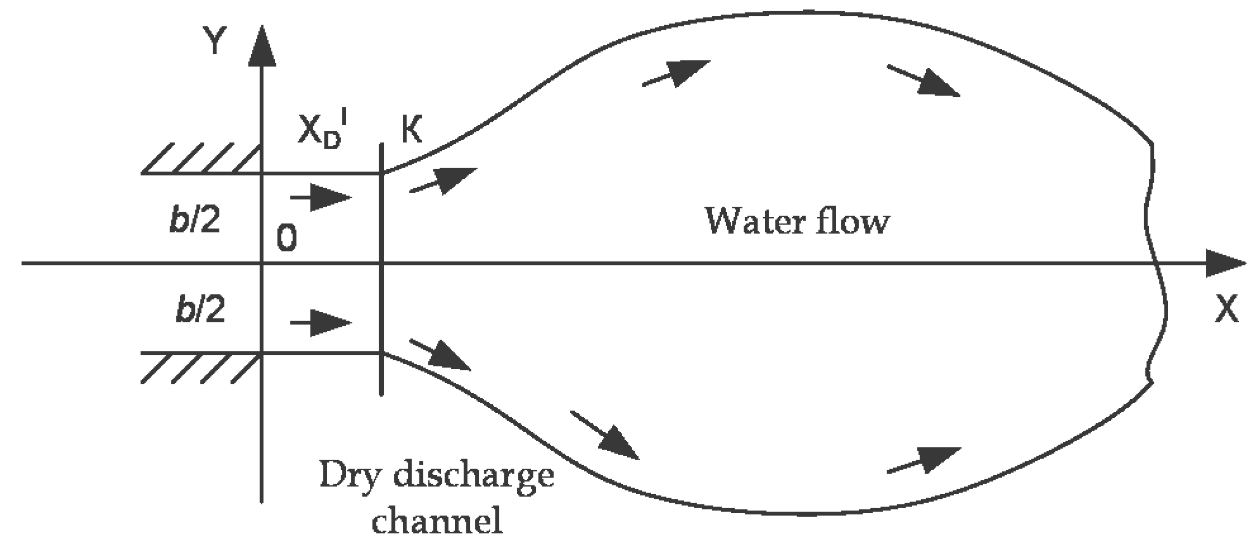
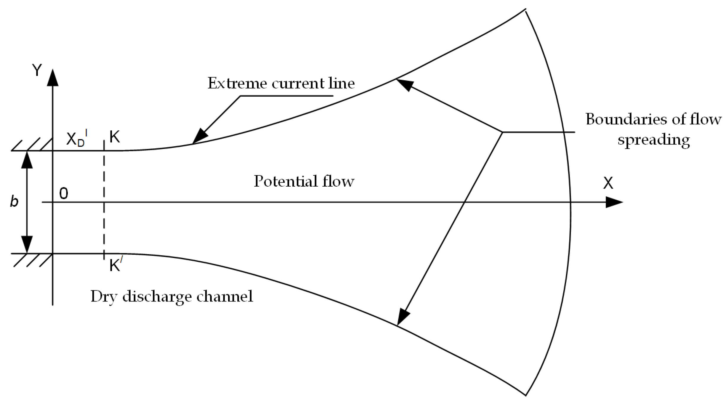
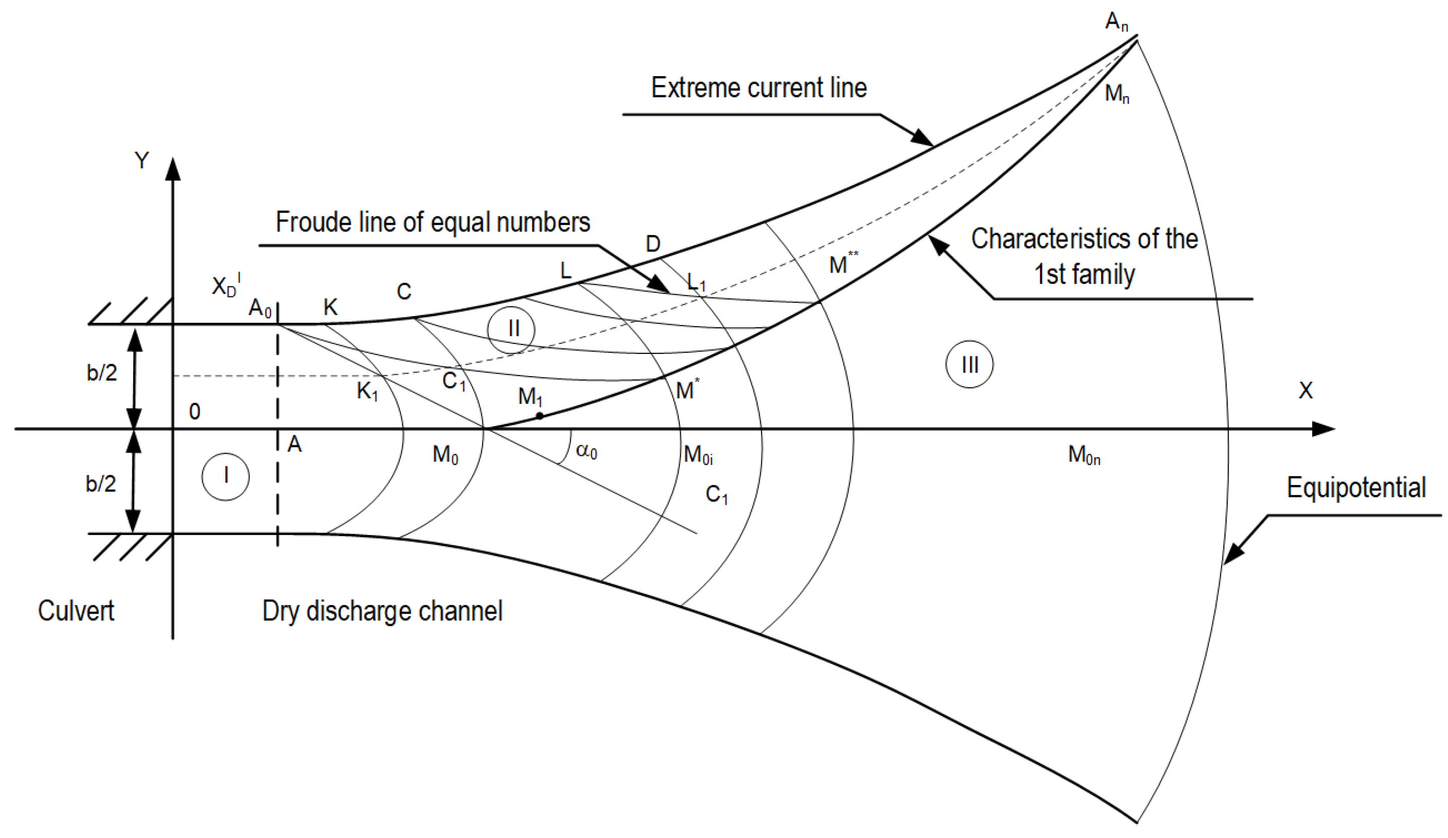
2.2. On the Boundary Problem of the Free Supercritical Flow behind an Unpressurised Culvert When It Spreads into a Wide Discharge Channel

The flow diagram of a real water flow (Figure 1), including drag forces, can be found in the reference manuals [1,2,22,23].
Scheme description. Water flows at high velocity from an unpressurised outlet into a wide diverting channel. Resistance forces to flow have the form [1]:
F r = K h α ,
where K, α depend on the selected flow resistance law and the roughness of the discharge channel bottom.
According to (7) the flow resistance forces increase as the depth of the flow decreases. Therefore, as a result of combined effect of gravity, inertia and flow resistance forces, the water flow becomes lobe shaped (confirmed by experiments).
From the experiments, field observations and published papers on supercritical flow [17,24,25,26,27,28], it can be argued that at the discharge of the flow from the pipe, there is a section of the flow, where the drag forces are small. As the flow resistance forces increase, the section turns into a still flow through a hydraulic jump and narrows in accordance with the general flow conditions of supercritical and calm flows [5,15].
The solution of determining the geometry of the flow distribution petal and the flow parameters within it will be shown in a later paper [17,29,30]. In this paper, we are going to study the flow spreading model in a simple case of the potential flow, as the base case, on which the real flow spreading model will be built.
Scheme of free flowing of potential supercritical flow behind unpressurized pipe in wide plain horizontal channel is shown in Figure 2.
At the discharge from the pipe, the flow parameters are as follows V 0 , h 0 , b: V 0 is a speed modulus; h 0 defines flow depth at the outlet of the pipe; b is pipe width; θ = 0 is the angle characterizing the flow velocity vector at its exit from the pipe;
F 0 2 = V 0 2 g h 0 > 1 —the flow is supercritical, i.e., high velocity.
There is a sharp curvature of the extreme current line in its small vicinity at point K, so from now on we will assume that at this point there is a discontinuity of the flow in its parameters.
We start solving the problem by solving it in the velocity hodograph plane. The authors in [13,26] found that the solution of the system (6) can be chosen as:
A sin θ τ 1 / 2 = ψ τ , θ ; A h 0 H 0 · cos θ τ 1 / 2 1 τ = φ τ , θ ;
1 3 < τ 0 τ 1 ,
where A is constant for the entire flow.
The version (8) may be applied to the problem, since for the extreme current line it follows from (8):
A sin θ τ 1 / 2 = V 0 b 2 ,
as the outermost current line detaches 50% of the total flow rate from the flow symmetry axis.
From (9) it follows that:
A = V 0 b 2 sin θ max ,
where θ max is an inclination angle of the velocity vector to the O X axis at τ = 1 [16].
Given (10), the equation for the outermost current line is converted to:
sin θ τ 1 / 2 = sin θ max .
Since it is known that supercritical flow, on entering expansion, widens, the angle θ must be a monotonically increasing function τ , and since the function τ 1 / 2 is also monotonically increasing, the ratio sin θ τ 1 / 2 can be made constant along the outermost line of the current. However, precisely at the point this design does not meet the boundary conditions τ = τ 0 , θ = 0 . Consequently, at the point · we assume flow discontinuity in its parameters (not continuity).
Proceeding from the continuity equation (Figure 3), separating elementary flow stream before and after it, taking into account Bernoulli integral, we obtain:
cos θ κ = τ κ 1 / 2 1 τ κ τ 0 1 / 2 1 τ 0
or
cos θ κ τ κ 1 / 2 1 τ κ = 1 τ 0 1 / 2 1 τ 0 .
Flow rate at the pipe outlet Δ Q 0 = b 0 · V 0 · h 0 .
Behind the pipe along the extreme current line Δ Q κ = b κ · V κ · h κ .
Given that V = τ 1 / 2 2 g H 0 , h = H 0 1 τ , we derive the Equation (11) from the condition Δ Q 0 = Δ Q κ .
Thus, Equation (11) indirectly confirms the validity of choosing the solution of the problem in the form (8).
The constant A is determined from the condition θ = θ max at τ = 1 , i.e., from the boundary condition, proceeding to the right (at infinity, meaning by infinity F r , τ 1).

2.3. Description of the Method for Solving the Problem in the Velocity Hodograph Plane

To solve (close) the problem in the velocity hodograph plane, it is necessary to determine the flow parameters at the point ·: τ = τ κ , θ = θ κ .
For this purpose, we first assume that a simple wave [5] is immediately adjacent to the area of uniform flow and the following equilibrium flow scheme is valid (8).
In the diagram in Figure 4, from point A 0 at an angle α 0 , a linear relationship of the 2nd family A 0 M 0 is drawn; M 0 M n is a linear relationship of the 1st family. The diagram is a pairing of a uniform flow I with a section of basic flow (unperturbed) or a general form III, of which II is a section of basic flow with flow discontinuity perturbations at point A.
If there were no discontinuities in the flow parameters, then the conjugate points on the characteristic of the 1st family M 0 M n , which passes through the entire flow via the points M 0 τ 0 , 0 and M n 1 , θ max with corresponding points on the outermost current line A 0 A n would pass through a simple wave.
In a simple wave, the characteristics of the 2nd family would be straight lines which would pass through the points on the characteristic of the 1st family.
The calculation by [31] showed that there was a satisfactory agreement with the experimental data for the first two steps, and then the discrepancy increased exponentially. To improve the accuracy the new mathematical model discussed in this paper is assumed which takes into account that only A 0 M 0 is a straight line, the remaining perturbation lines degenerate into the lines of equal Froude numbers. Section II is therefore a section with perturbation lines—lines of equal Froude numbers A M * , L M * * , etc.). The subsequent calculation according to the corrected program [32] confirmed the correctness of this assumption and good convergence of the calculated and experimental data.
In the velocity hodograph plane, this section has the parameters:
τ = τ 0 = V 0 2 2 g H 0 ; θ = θ 0 = 0 ;
The characteristics of the 1st family M 0 M n passes through the points M 0 with parameters τ 0 , θ = 0 and M n with parameters τ = 1 , θ = θ max .

2.3.1. Solving the Problem in the Uniform Flow Area (Section I)

In section I, the solution to this problem consists of determining the geometry and parameters of the flow and consists of several steps.
  • Since at M 0 the flow velocity and the parameter τ 0 , then the lines angle α 0 is also determined at this point:
    α 0 = arcsin 1 τ 0 2 τ 0 ,
    and consequently, the direction of the rectilinear characteristic of the 2nd family— A 0 M 0 .
  • Knowing the length of the inertial front [33,34,35,36,37], the geometry of the uniform flow section can be determined.
    X D I = t r u n c F 0 1 sin θ max F 0 + 2 h 0 + 1 c m ,
    X D I —front length of the inertial section along the flow symmetry axis O X .
    The geometry of section I is determined by the parameters X D I , α 0 = arcsin 1 τ 0 2 τ 0 , and pipe width b.
    Since the flow in area I is uniform, then τ = τ 0 , θ = 0 , V = V 0 , h = h 0 .
  • Let us determine parameter values τ , θ on the characteristic of the 1st family. From the characteristic equation of the 1st family [20,38], the angle θ can be determined at the known τ τ 0 , 1
    θ ( τ ) = 3 · a r c t g 3 τ 1 3 1 τ a r c t g 3 τ 1 1 τ + C 1 ,
    where
    C 1 = a r c t g 3 τ 0 1 1 τ 0 3 · a r c t g 3 τ 0 1 3 1 τ 0 .
    Setting the spacing Δ τ = 1 τ 0 N , we get:
    τ i = τ 0 + i Δ τ
    θ i is determined from (12) at a fixed N.
    The angle θ max is also determined from the system of Equation (12).
  • Let us determine the flow coefficients at the intersection points i of the current line with the characteristic of the 1st family. From the equation equitable along the current line
    sin θ τ 1 / 2 = K sin θ max
    subject to certain parameters θ i , τ i from (12) the flow coefficient K i between this current line and the longitudinal axis of flux symmetry OX is determined.
    K i = sin θ i τ 1 / 2 sin θ max .
Wave angle at the point θ i , τ i can be determined by a well-known formula [5]:
α i = a r c t g 1 τ i 2 τ i .

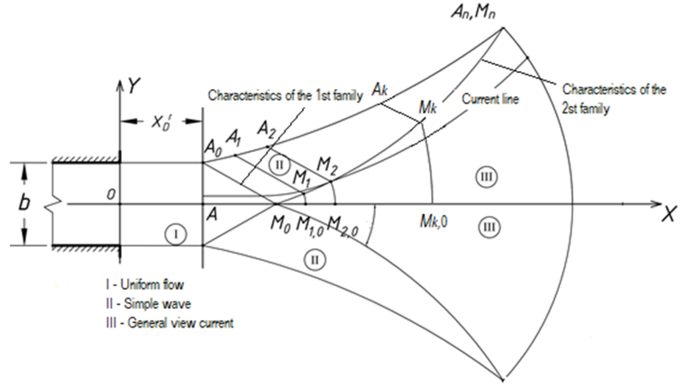
2.3.2. Problem Solving in the General Flow Area (Section III)
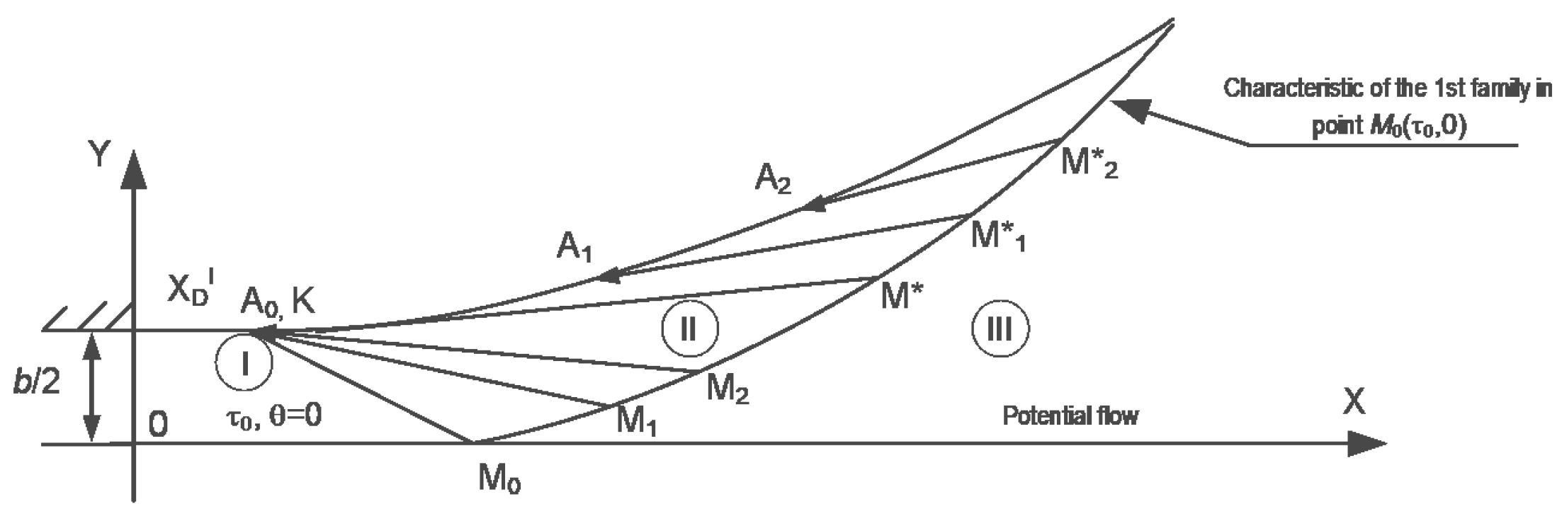
  • Let us define the parameters τ , θ in the flow area of section III. The base flow is given by the equations in the velocity hodograph plane (Figure 5):
    ψ = A sin θ τ 1 / 2 ; φ = A h 0 H 0 · cos θ τ 1 / 2 1 τ .
    This section is bounded by the 1st family characteristic and the flow symmetry axis O X . The characteristic runs through a point M 0 with parameters τ = τ 0 ; θ = 0 . This is the main flow characteristic that runs through the entire flow. It has the form [20]:
    θ = 3 · a r c t g 3 τ 1 3 1 τ a r c t g 3 τ 1 1 τ + C 1 ,
    where
    C 1 = a r c t g 3 τ 0 1 1 τ 0 3 · a r c t g 3 τ 0 1 3 1 τ 0 .
  • Setting the parameters θ i , τ i at the points of intersection of the characteristics of the 1st family and the corresponding current line, it is possible to determine the parameters of the intersection points i of the current line and j of the equipotentiality from the system
    sin θ i j τ i j 1 / 2 = K i sin θ max ; cos θ i j τ i j 1 / 2 1 τ i j = cos θ i τ i 1 / 2 1 τ i .
    Herewith
    τ 0 τ i j 1 ; θ θ i j θ max .
  • Coordinates of the points x i j , y i j in region III of the flow is determined from the differential relation (5).
    If moving along the corresponding current line, Equation (5) by virtue of the condition d φ = 0 is recomposed after separating the variables in the form of:
    d x = d φ cos θ τ 1 / 2 2 g H 0 ; d y = d φ sin θ τ 1 / 2 2 g H 0 .
    Expressing the differential d φ and the angle θ by τ , using the links along the current line and integrating Equation (13), the coordinates of the points with the parameters θ i j , τ i j and this was described in the monographs [18,20].
  • Determination of parameters at points C 1 , L 1 . Let us draw the equipotential through the point C. Then the equation of the equipotential passing through the point C:
    cos θ C τ C 1 / 2 1 τ C = cos θ C 1 τ C 1 1 / 2 1 τ C 1 .
    At point C 1 we assume τ C 1 = τ * . Consequently,
    cos θ C 1 = cos θ C · τ C 1 1 / 2 1 τ C 1 τ C 1 / 2 1 τ C .
    θ C 1 = arccos θ C 1 .
    Alternatively,
    sin θ C 1 = 1 cos 2 θ C 1 ; θ C 1 = arcsin 1 cos 2 θ C 1 .
    Similarly, we determine the parameters at the point L 1 .
  • Determining the coordinates of the points C 1 , L 1 . Parameters at a point C 1 are τ C 1 , θ C 1 .
    The equation of the current line passing through the point C 1 :
    sin θ C 1 τ C 1 / 2 = K sin θ max .

2.3.3. Determination of Flow Parameters in the Simple Wave Region (Section II)

A simple current wave in section II, bounded by the uppermost current line and the characteristic of the first family, passing through the point M 0 .
  • We determine t g θ + α as an angular coefficient of slope of the tangent to the 1st family characteristic t g θ + α = f * τ and a section of its uniformity. Since t g θ + α is a monotonically increasing function of the argument τ , then we determine the monotonicity areas of the function:
    f τ = θ + α = θ τ + α τ ,
    where
    θ τ = 3 · a r c t g 3 τ 1 3 1 τ a r c t g 3 τ 1 1 τ + C 1 ; α τ = arcsin 1 τ 2 τ .
    To do this, we solve the equation
    f τ = θ τ + α τ = 0 .
    Root of the Equation (14) τ = τ * defines areas of uniformity of the function f τ , and consequently the functions f * τ :
    τ 0 , τ * , τ * , 1 .
    At the site τ 0 , τ * the function f * τ monotonically decreases, and in the area τ * , 1 monotonically increases.
  • Similarly, to section II with simple waves, we connect the Froude line points M * and A of equal numbers A M * , the line on which is τ = τ * , and the angle θ is determined from the solution to the problem.
    Equal Froude number lines convey perturbations in the presence of discontinuities in the flow parameters.
  • From the equation of the extreme current line determine the angle
    θ A * = arcsin τ * 1 / 2 sin θ max .
    As t g θ increases ultimately along the extreme current line A C L A n , the points A and M * can be connected by Froude’s equal number perturbation waves.
    Perturbations by equal Froude number lines are more generic disturbances than a simple wave. In a simple wave
    θ = c o n s t A , τ = c o n s t A .
    In a wave of Froude equal numbers line τ = c o n s t .
    Point M * should necessarily be connected to point A, as the minimum possible value at point A must be τ = τ * and further increase downstream.
  • Further conducting an equipotential M 0 C , let us determine the flow parameters at point C by solving the system:
    cos θ C τ C 1 / 2 1 τ C = 1 τ 0 1 / 2 1 τ 0 ; sin θ C τ C 1 / 2 = sin θ max .
    Similarly, we determine the flow parameters at the point L:
    sin θ L τ L 1 / 2 = sin θ max ,
    assuming (15) τ L = τ * * , where τ * * is a parameter at a characteristic point M * * , for which the following equation is true:
    θ τ * * = τ * * .
  • Choice of steps in sections: Step selection Δ τ 1 on a characteristic M 0 M n between the points M 0 and M * :
    Δ τ 1 = τ * τ 0 N 1 .
    Then,
    τ i = τ 0 + Δ τ 1 · i ; i = 0 , 1 , 2 , , N 1 .
    Selecting the sampling step Δ τ 2 between the points M * and M * * :
    Δ τ 2 = τ * * τ * N 2 .
    Then,
    τ j = τ * + Δ τ 2 · j ; j = 0 , 1 , 2 , , N 2 .
    Selecting the sampling step Δ τ 3 between the points M * * and M n ( τ ) :
    Δ τ 3 = 1 τ * * N 3 .
    Then,
    τ k = τ * * + Δ τ 3 · k ; k = 0 , 1 , 2 , , N 3 .
  • The right lines A 0 M 0 , A 1 M 1 in a simple wave are determined from the condition that the characteristic of the 2nd family passes through the point A i and has an angular coefficient t g θ i α i [5]. Extreme current line points A i are determined by the distance ρ i on the corresponding line M i A i :
    ρ i = b 1 K i τ 0 1 τ 0 2 τ i 1 τ i sin α i ,
    the flow rate between the outermost current line and the longitudinal axis of flow symmetry is maintained. It is equal to half of the total flow rate.
Based on the proposed theory, an algorithm and a PC software has been developed which gives adequate results.

2.3.4. Improvement of the Proposed Algorithm

The presented theory and algorithm can be somewhat improved in the following way.
Based on the calculation results, it is found that the function θ i + α i of τ i is not uniformly monotonous at τ 0 τ i 1 , and it defines a tangent t g θ i + α i to the characteristic of the 1st family and the values θ i , τ i along a simple wave connecting the points A i and M i .
It has been found that the function θ i + α i decreases monotonically to τ = τ * and further increases monotonically τ = τ * which corresponds to the point M * .
It has also been revealed that the bundle of centered lines exits from a point A 0 at the points M 1 , M 2 , , M * .
It is also revealed that due to the hydraulic jump at the point A 0 by the parameters τ , θ the characteristic of the 1st family and the upper-most line of the current cascade cannot be matched by simple waves. The right lines A i M i degenerate into lines of equal Frood numbers:
τ = c o n s t .
Thus, the concept of a <<simple wave>> can be extended to the concept of a <<Froude equal numbers wave>>. Apparently, along the line F r = c o n s t , τ = c o n s t , V = c o n s t , h = c o n s t follow.
If the condition is added to the Froude equal numbers line θ = c o n s t , then it transforms into a simple wave. The <<simple wave>> lines are converted to <<equal Froude number lines>> when there are hydraulic jumps in the flow, as described in this paper.
As a consequence of this, the schematic in Figure 4 can be replaced by the following schematic (Figure 6).
The flow parameters in this scheme vary uniformly downstream from point A 0 along the extreme current line (confirmed by experiments), and the disturbance lines are the lines of equal Froude numbers. These connect the corresponding points between the uppermost current line and the first family characteristic.
According to this scheme the section:
I—zone of uniform flow;
III—zone of basic flow;
II—perturbation transmission area via equal Froude number lines: A i M i * .
The algorithm for calculating the parameters of the upper-most current line in this case is as follows:
– the point on the characteristic of the 1st family M * in which the functions f τ = θ + α take a minimum is numerically determined. Let us denote it by τ * , the corresponding value θ by θ * .
Then the equation for the extreme current line will be true for τ * τ 1 , θ A θ θ max .
The equation in the velocity hodograph plane for the extreme upper current line:
sin θ τ 1 / 2 = sin θ max .
counts at the point A 0 τ = τ * . Then
θ A = arcsin τ * 1 / 2 sin θ max .
Thus, going further to the physical plane of flow, using the complex relationship between the planes Φ x , y = G τ , θ by the method described in the article and monographs [18,20], we determine the coordinates of the outermost current line and the velocity and depth values along it.

3. The Discussion of the Results

Let us consider a flow with the following parameters:
  • initial flow velocity V 0 [cm/s];
  • initial depth of the flow relative to the bottom h 0 [cm];
  • gravity acceleration g = 981 [cm/s 2 ];
  • pipe width b [cm].
Flow coordinates are obtained from the field experiment
X E = 0 4 24 44 64 71 T ; Y E = b / 2 9.5 38 59 76 80 T .

3.1. Solving the Problem in the Uniform Flow Area (Section I)

Using the algorithm above, we find:
  • Froude number F 0 = 2.4 ;
  • initial flow velocity V 0 = Q h 0 b = 147.654 cm/s;
  • hydrodynamic head H 0 = 20.382 cm;
  • initial flow kinetics (block 1, item 4) τ 0 = 0.545 ;
  • wave angle at the point where the flow exits the pipe α 0 = 0.702 p or α 0 = 40 23 ;
  • angle of the velocity vector of the liquid flow to the OX axis at infinity θ max = 0.981 p or θ max = 56 23 ;
  • length of inertial front X D I = 3 cm;
  • distance from the end of the inertial section to the point along the flow symmetry axis M 0 A M 0 = 9.457 cm;
  • the length of the straight-line segment of the 2nd family characteristic between the points A 0 and M 0
    A 0 M 0 = 12.387 cm.
Let us break down the kinetic flow parameter from τ 0 to 1 for 10 spacings. Step length Δ τ = 0.051 .
Table 1 shows calculated values for flow abscissa, flow velocity and depth.
The equipotential can be highlighted by a specific parameter value τ on the flow symmetry axis. By setting the parameter τ 0 to the point M 0 on the flow symmetry axis it can be possible to determine the parameters θ τ C , C followed by the coordinates x C y C of—point on the outermost current line. Then by changing the kinetic parameter (e.g., with a constant step) we obtain a set of extreme current line points. The numerical experiment was to calculate the values of kinetics parameter, angle of slope of flow velocity vector to symmetry axis and coordinates of points on the extreme line of current with abscissa on symmetry axis. Calculation results are summarized in Table 2.
The calculation results for the last column of Table 2 show good convergence of the algorithm with the experimental data, Given in the dissertation work of Kokhanenko V.N. [17].

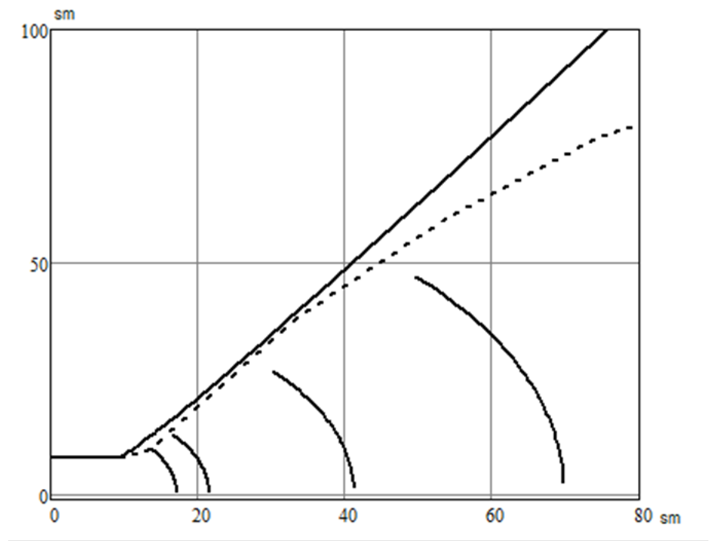
3.2. Problem Solution in the General Flow Area (Section III) and in the Simple Wave Area (Section II)

Kinetics parameter at point A 0 on the outermost current line τ * = 0.6667 . The found value τ * is constant on the line A 0 M * the line of constant Froude numbers.
Angle of inclination of the flow velocity vector at the point A can be θ A = 0.746 p or θ A = 42 74.
Parameters in the velocity hodograph plane of point C of the intersection of equipotentialism with the current ruler and passing through the point M 0 : τ C = 0.719 , θ C = 0.782 p or θ C = 44 82.
Let us set 35 points on the characteristic M 0 M n between points M 0 and M * . Then the step is equal to Δ τ 1 = 9.7·10 3 . The kinetic parameter, the inclination angle of the liquid velocity vector to the OX axis and the flow coefficients at these points are given in Table 3.
The parameter grid in area III can now be constructed. The current line is given by the flow coefficients and the equipotential by the kinetic parameter. Next, the coordinates of the points in the general view area and at the far end of the current line are determined using the parameters obtained. Figure 7 shows a diagram of the outermost current line and some equipotentials. For comparison, the same figure shows a plot of the extreme current line obtained experimentally.

4. Conclusions

In this paper, a new method of calculating parameters of free-flow supercritical potential flow behind rectangular non-pressure outlets has been proposed.
It has been proved theoretically and practically by means of calculation results that pairing of uniform flow with the flow of general form (12) should be carried out by means of perturbation lines in the form of Froude equal number lines.
To solve the nonlinear system of differential equations in the new calculation method, an auxiliary virtual plane of the velocity hodograph and its coupling equations to the main characteristic of the 1st family in the physical plane are used.
Transition to the physical plane is implemented at the point M* of change of the monotonicity sign, which allowed us to obtain an analytic solution of the overall problem in terms of the current line, equipotential and the virtual plane of the velocity hodograph.
Further development of the method will make it possible to obtain a series of graphs for various Froude numbers at the pipe outlet and to improve the universal graph by I.A. Sherenkov [28].

Funding

This research received no external funding.

Data Availability Statement

The data presented in the article do not require copyright. They are freely available and are listed at the reference address in the bibliography.

Acknowledgments

The authors express their gratitude to the reviewers for valuable comments, who allowed us to improve the content of the article, and to the editors of the journal for their positive attitude towards our work.

Conflicts of Interest

The author declares no conflict of interest.

References

  1. Bolshakov, V.A. Hydraulics, 2nd ed.; Higher School: Kiev, Ukraine, 1984. [Google Scholar]
  2. Shterenlicht, D.V. Hydraulics, 3rd ed.; Kolos: Moscow, Russia, 2005. [Google Scholar]
  3. Volchenkova, G.Y. Manual for Hydraulic Calculations of Small Culverts; All-Russian Research Institute of Transport Construction, Main Directorate for Design and Capital Construction of the USSR Ministry of Transport: Moscow, Russia, 1992. [Google Scholar]
  4. Bernadsky, N.M. The theory of supercritical flow and its application to the construction of the plan of currents in open water bodies. In Materials on Hydrology, Hydrography and Water Forces of the USSR; Gosenergoizdat: Moscow-Leningrad, Russia, 1993; p. 20. [Google Scholar]
  5. Yemtsev, B.T. Two-Dimensional Stormy Flow; Energy: Moscow, Russia, 1967. [Google Scholar]
  6. Vysotsky, L.I. Management of Stormy Flows at Spillways; Energy: Moscow, Russia, 1990. [Google Scholar]
  7. Loytsyansky, L.G. Mechanics of Liquid and Gas, 5th ed.; Nauka: Moscow, Russia, 1978. [Google Scholar]
  8. Orlov, V.; Gasanov, M. Exact Criteria for the Existence of a Moving Singular Point in a Complex Domain for a Nonlinear Differential Third-Degree Equation with a Polynomial Seventh-Degree Right-Hand Side. Axioms 2022, 11, 222. [Google Scholar] [CrossRef]
  9. Orlov, V.; Gasanov, M. Existence and Uniqueness Theorem for a Solution to a Class of a Third-Order Nonlinear Differential Equation in the Domain of Analyticity. Axioms 2022, 11, 203. [Google Scholar] [CrossRef]
  10. Orlov, V.; Gasanov, M. Analytic Approximate Solution in the Neighborhood of a Moving Singular Point of a Class of Nonlinear Equations. Axioms 2022, 11, 637. [Google Scholar] [CrossRef]
  11. Orlov, V.; Gasanov, M. Technology for Obtaining the Approximate Value of Moving Singular Points for a Class of Nonlinear Differential Equations in a Complex Domain. Mathematics 2022, 10, 3984. [Google Scholar] [CrossRef]
  12. Korn, G. Mathematics for Scientists and Engineers; Nauka: Moscow, Russia, 1970. [Google Scholar]
  13. Aleksandrova, M.S. Method of Analogies between Hydraulics of Two-Dimensional Water Flows and Gas Dynamics. Constr. Archit. 2020, 2, 49–52. [Google Scholar] [CrossRef]
  14. Popov, D.N.; Panaiotti, S.S.; Ryabinin, M.V. Hydromechanics; Bauman Moscow State Technical University: Moscow, Russia, 2002. [Google Scholar]
  15. Esin, A.I. Problems of Technical Fluid Mechanics in Natural Coordinates; Saratov SAU: Saratov, Russia, 2003. [Google Scholar]
  16. Bolshakov, V.A.; Galetskiy, V.I.; Denisenko, I.D. Water accounting for automated regulation of water supply to canals. Melior. Water Manag. 1983, 3, 18–24. [Google Scholar]
  17. Kokhanenko, V.N. Two-Dimensional in Plan Stormy Stationary Flows behind the Culverts in Conditions of Free Spreading, Autor’s Abstract. Ph.D. Thesis, Diss. Doct. Tech. Science.. Moscow State University of Civil Engineering, Moscow, Russia, 17 June 1997. [Google Scholar]
  18. Kokhanenko, V.N. Modeling of One-Dimensional and Two-Dimensional Open Water Flows; Publishing House of the Southern Federal University: Rostov-on-Don, Russia, 2007. [Google Scholar]
  19. Chaplygin, S.A. Mechanics of liquid and gas. In Maths. General Mechanics: Selected Works; Nauka: Moscow, Russia, 1976. [Google Scholar]
  20. Kohanenko, V.N.; Volosukhin, Y.V. Modeling of Stormy Two-Dimensional in Terms of Water Flows; Publishing House of the Southern Federal University: Rostov on Don, Russia, 2013. [Google Scholar]
  21. Kohanenko, V. Derivation of the main system of motion equations for a two-dimensional flow in the velocity hodograph plane and the search for its particular solutions. The manuscript was deposited with the All-Russian Institute of Scientific and Technical Information of the Russian Academy of Sciences (VINITI). Russia, 1996; Volume 96, 98. [Google Scholar]
  22. Kajishima, T.; Taira, K. Computational Fluid Dynamics—Incompressible Turbulent Flows; Springer: Berlin/Heidelberg, Germany, 2016. [Google Scholar]
  23. William, E.B.; Richard, C.D.; Douglas, B.M. Elementary Differential Equations and Boundary Value Problems; John Wiley & Sons: Hoboken, NJ, USA, 2021. [Google Scholar]
  24. Sherenkov, I.A. The spreading of a stormy flow behind the outlet heads of culverts under railway embankments. Proc. Kharkov Inst. Railw. Eng. Named After S. M. Kirov 1957, 30. [Google Scholar]
  25. Sherenkov, I.A. On the planned problem of spreading a jet of a turbulent flow of an incompressible liquid. News Acad. Sci. USSR 1958, 1, 72–78. [Google Scholar]
  26. Sherenkov, I. Experimental study of the supercritical flow spreading behind the outlet heads of culverts. In Proceedings of the Joint Seminar on Hydraulic Engineering and Water Management Construction, Kharkov, Ukraine; 1958; Volume 1. [Google Scholar]
  27. Sherenkov, I.A. On the Role of Normal Supercritical Stresses in the Currents Plan Formation Hydraulics and Hydraulic Engineering; Technics: Kiev, Ukraine, 1973; Volume 17. [Google Scholar]
  28. Sherenkov, I.A. Applied Planning Tasks of Gravity Flows Hydraulics; Energy: Moscow, Russia, 1978. [Google Scholar]
  29. Kokhanenko, V.N. On the planned problem of spreading a supercritical flow of incompressible liquid. Sci. J. Bull. High. Educ. Institutions North Cauc. Reg. Tech. Sci. 2012, 6, 82–88. [Google Scholar]
  30. Duvanskaya, E.V. Calculation of the Potential Movement of Two-Dimensional Stationary, Quiet Flows. Ph.D. Thesis, Diss. Cand. Tech. Sciences.. Novocherkassk State Reclamation Academy, Novocherkassk, Russia, 25 September 2003. [Google Scholar]
  31. Kokhanenko, V.N. Determination of Parameters of a Freely Spreading Flow. Certificate of Registration of Computer Programs, Federal Institute of Industrial Property (FIPS) No. RU 2022618552. 2022. Available online: https://www1.fips.ru/ofpstorage/Doc/PrEVM/RUNWPR/000/002/022/618/552/2022618552-00001/ (accessed on 1 July 2022).
  32. Kokhanenko, V.N.; Kelekhsaev, D.B. The problem solution of determining the extreme streamline equation and parameters along it, taking into account the XD section. In Research Results—2019: Materials of the IV National Conference for Teaching Staff and Scientific Workers; SRSPU (NPI): Novocherkassk, Russia, 2019; pp. 113–117. [Google Scholar]
  33. Kokhanenko, V.N.; Kelekhsaev, D.B.; Kondratenko, A.I.; Evtushenko, S.I. Two-dimensional motion equations in water flow zone. IOP Conf. Ser. Mater. Sci. Eng. 2019, 698, 066026. [Google Scholar] [CrossRef]
  34. Kokhanenko, V.N.; Kelekhsaev, D.; Kondratenko, A.; Evtushenko, S. A System of Equations for Potential Two-Dimensional In-Plane Water Courses and Widening the Spectrum of Its Analytical Solutions. AIP Conf. Proc. 2019, 2188, 050017. [Google Scholar] [CrossRef]
  35. Kokhanenko, V.N.; Kelekhsaev, D.B.; Kondratenko, A.I.; Evtushenko, S.I. Solution of equation of extreme streamline with free flowing of a torrential flow behind rectangular pipe. IOP Conf. Ser. Mater. Sci. Eng. 2020, 775, 012134. [Google Scholar] [CrossRef]
  36. Kokhanenko, V.N.; Kelekhsaev, D.B.; Kondratenko, A.I.; Evtushenko, S.I. Solution of Equations of Motion of Two-Dimensional Water Flow. Constr. Archit. 2019, 7, 5–12. [Google Scholar] [CrossRef]
  37. Kokhanenko, V.N.; Burtseva, O.A.; Evtushenko, S.I.; Kondratenko, A.I.; Kelekhsaev, D.B. Two-Dimensional in Plan Radial Flow (NonPressure Potential Source). Constr. Archit. 2019, 7, 25. [Google Scholar] [CrossRef]
  38. Vysotsky, L.I. Hydraulic Calculation of Scattering Trampolines by the Method of Longitudinal Approximations; MCEU Named after V. V. Kuibyshev: Moscow, Russia, 1960. [Google Scholar]
Figure 1. Schematic of a real flow spread.
Axioms 12 00011 g001
Figure 2. Schematic of a potential supercritical flow behind an unpressurised pipe into a wide, plain horizontal channel.
Axioms 12 00011 g002
Figure 3. Elementary flow before and after exiting the pipe.
Axioms 12 00011 g003
Figure 4. Flow spread diagram.
Axioms 12 00011 g004
Figure 5. Flow spread diagram to the new mathematical model.
Axioms 12 00011 g005
Figure 6. Schematic for calculating the flow parameters.
Axioms 12 00011 g006
Figure 7. Plots of extreme current line and some equipotentials (solid) obtained from numerical calculations and extreme current line obtained from in situ experiments (dashed).
Axioms 12 00011 g007
Table 1. Kinetics values τ i , flow abscissa X i 0 , its velocity V i 0 and depth h i 0 at the symmetry axis points.
τ i 0.5450.5960.6460.6970.7470.7980.8480.8990.9491
X i 0 6.2997.2698.54710.25912.64216.16921.94233.24466.3363233
V i 0 147.654154.345160.759166.926172.873178.622184.192189.599194.855199.963
h i 0 9.2748.2347.2156.1765.1574.1173.0982.0591.0390
Table 2. Calculation of extreme line flow point ordinates and comparison with experimental data.
Point No.Abscissa on the Symmetry Axis at X 0 i Parameter of Kinetics, τ C i Angle of Inclination of the Flow Velocity Vector to the Axis of SymmetryFlow Ordinates on the Extreme LineExperimental Data at Some PointsRelative Algorithm Error, %
100.5450.661880
240.7670.81510.442115.073
380.8660.88413.637
4120.9080.91418.687
5160.9310.9323.973
6200.9450.9429.402
7240.9540.94734.926388.090
8280.9610.95240.519
9320.9660.95646.162
10360.970.95951.846
11400.9730.96157.56
12440.9750.96363.3597.288
13480.9780.96569.06
14520.9790.96674.84732.458
Table 3. Kinetics, slope angle of the fluid velocity vector to the OX axis and flow coefficients at the points on the characteristic M 0 M n (area III).
Step No.KineticsAngle of Inclination of Velocity VectorFluid Flow Coefficient
10.54520.1450.212
20.57560.1570.229
30.60590.170.246
40.63630.1840.263
50.66670.1970.28
60.67650.2110.297
70.68620.2240.314
310.92080.6970.788
320.93060.7340.819
330.94040.7780.853
340.95010.8340.896
350.95990.9370.97
Disclaimer/Publisher’s Note: The statements, opinions and data contained in all publications are solely those of the individual author(s) and contributor(s) and not of MDPI and/or the editor(s). MDPI and/or the editor(s) disclaim responsibility for any injury to people or property resulting from any ideas, methods, instructions or products referred to in the content.

