Efficient Modified Meta-Heuristic Technique for Unconstrained Optimization Problems

Abstract

In this paper, a new Modified Meta-Heuristic algorithm is proposed. This method contains some modifications to improve the performance of the simulated-annealing algorithm (SA). Most authors who deal with improving the SA algorithm presented some improvements and modifications to one or more of the five standard features of the SA algorithm. In this paper, we improve the SA algorithm by presenting some suggestions and modifications to all five standard features of the SA algorithm. Through these suggestions and modifications, we obtained a new algorithm that finds the approximate solution to the global minimum of a non-convex function. The new algorithm contains novel parameters, which are updated at each iteration. Therefore, the variety and alternatives in choosing these parameters demonstrated a noticeable impact on the performance of the proposed algorithm. Furthermore, it has multiple formulas by which the candidate solutions are generated. Diversity in these formulas helped the proposed algorithm to escape a local point while finding the global minimizer of a non-convex function. The efficiency of the proposed algorithm is reported through extensive numerical experiments on some well-known test problems. The performance profiles are used to evaluate and compare the performance of our proposed algorithm against the other five meta-heuristic algorithms. The comparison results between the performance of our suggested algorithm and the other five algorithms indicate that the proposed algorithm is competitive with, and in all cases superior to, the five algorithms in terms of the efficiency, reliability, and effectiveness for finding the global minimizers of non-convex functions. This superiority of the new proposed algorithm is due to those five modified standard features.

1. Introduction

The main aim of this paper is to find the global minimizer of the objective function of an unconstrained problem that is defined by:

$$\underset{x\in R^n}{min}f\left(x\right),$$

(1)

where the function f is assumed to be continuous.

Several practical applications of global optimization problems arise in different fields, such as technical sciences, industrial engineering, economics, operations research, networks, chemical engineering, etc. See, for example, [1,2,3,4,5,6,7,8,9,10,11].

Therefore, many new problems are being generated continuously. These problems need to be solved. A mathematical modeling process is an important tool that is used to formulate them as mathematical problems. The result is that these problems are formulated as unconstrained, constrained and multi-objective optimization problems.

The unconstrained optimization problems grow immediately in several practical applications [12]. Therefore, these problems have attracted the attention and concerns of many researchers for suggesting many algorithms that solve these problems, see, for example, [13,14,15,16,17].

Finding the global minimum of the function f is far more difficult—analytical methods are frequently not applicable, and the use of numerical solution algorithms often leads to challenges.

Therefore, there has been a great development in optimization algorithms that are designed to deal with these problems. The ideas of those proposed methods depend on the principle of meta-heuristic strategies (stochastic methods). There are different classifications for meta-heuristic methods [18].

Mohamed et al. [7] presented a brief description of these classifications, such as nature-inspired against non-nature-inspired, single-point search versus population-based, static objective function against dynamic objective function, different neighborhoods against one single neighborhood and memory usage versus memory fewer methods. In stochastic methods, the minimization process depends partly on probability.

In contrast, in the deterministic methods, no probabilistic information is used [19].

The numerical global optimization algorithms are capable of approximating the optimal solutions to these problems. The main feature of the global optimization methods is to prevent convergence to local optima and increase the probability of finding the global optimum [19].

Therefore, for finding the global minimum of the unconstrained problem by using deterministic methods, it needs an exhaustive search over the feasible region of the function f and additional assumptions on the function f. On the antithesis of that, to approximate the global minimum of the unconstrained problems using stochastic methods, the asymptotic convergence probability can be proved, i.e., these methods are asymptotically effective with a probability of 1; see, for example, [20,21,22].

Hence, the computational results of the stochastic methods are better than those of the deterministic methods [23].

Therefore, a meta-heuristics strategy (stochastic method) is used to guide the search process [23]. Thus, the meta-heuristic is a technique designed for solving a problem more quickly when classic methods are too slow, or for finding an approximate solution when classic methods fail to find any exact or near-exact solution. This is achieved by trading optimality, completeness, accuracy or precision for speed [18,24,25].

The simulated-annealing algorithm (SA) is considered one of the most successful meta-heuristic strategies and has been developed to be capable of dealing with many problems in different fields. However, the process of developing and improving the SA algorithm is still open in order to gain the advantages of this method and overcome its drawback. Indeed, the numerical results demonstrate that the simulated-annealing technique (SA) is very efficient and effective for finding the global minimizer. See, for example, [3,9,26,27,28,29].

The SA has a major advantage of being able to avoid getting trapped at a local minimum [30,31].

In the rest of this section, we present a historical survey of some developments on the simulated-annealing algorithm, which is proposed by many authors.

Metropolis et al. [32] suggested an algorithm to numerically find equilibrium distribution, which is known as the Metropolis Algorithm (MA). SA is a sequence of MA. They applied the algorithm to simulate the behavior of physical systems in the presence of a heat bath, for finding the equilibrium configuration of a collection of atoms at a given temperature. Since that date, various developments and suggestions were presented by many authors. Kirkpatrick et al. [33] linked the simulated-annealing algorithm (SA) of solids with combinatorial discrete minimization problems. Vanderbilt and Louie [34] and Bohachevsky et al. [35] modified the simulated-annealing method for continuous variable problems. Anily and Federgruen [36] provided probabilistic analysis of different designs of simulated-annealing algorithms to prove a convergence for the simulated-annealing algorithm with general acceptance probability functions. Corona et al. [30] proposed an adaptive method of the simulated annealing for continuous optimization problems. Dekkers and Aarts [31] presented a stochastic approach to address global optimization based on the simulated-annealing algorithm, which is similar to the formulation of the simulated annealing applied to discrete optimization problems. They also proved asymptotic convergence to the set of global minimizers. Ingber [37] introduced a study about the advantages and disadvantages of the simulated-annealing method. Bertsimas et al. [38] described the simulated-annealing algorithm, its convergence and its behavior in an application. Goffe et al. [39] presented some improvements to the simulated-annealing algorithm as an extension to Corana’s algorithm. Tsallis and Stariolo [40] presented a generalized simulated-annealing algorithm for finding the global minimum of a continuous function. Siarry et al. [41] introduced some suggestions for the simulated-annealing algorithm to solve highly multimodal functions of 2 to 100 variables. Nouraniy and Andresenz [42] presented a comparison of the cooling strategies for the simulated-annealing algorithms. In the study, the authors compared different proposed cooling schedules in order to find the best cooling strategy.

A self-learning simulated-annealing algorithm is presented by [43]. It is developed by combining the characteristics of the simulated annealing and the domain elimination methods. Ali et al. [44] proposed various simulated-annealing algorithms for optimization involving continuous variables. Bouleimen and Lecocq [45] presented simulated annealing adaptations for the resource-constrained project scheduling problem (RCPSP) and its multi-mode version. Ali and Gabere [46] presented a simulated annealing driven multi-start algorithm for continuous global optimization. They also studied the convergence properties of their algorithm and test its performance on a set of 50 problems.

Wang et al. [47] proposed a new improved meta-heuristic simulated-annealing-based krill herd (SKH) method for global optimization. Rere et al. [48] proposed a simulated annealing to improve the performance of convolution neural network (CNN), as an alternative approach for optimal deep learning (DL) using a modern optimization technique.

Certa et al. [49] proposed a new innovative cooling law for simulated-annealing algorithms. Poorjafari et al. [29] presented a study to compare the genetic algorithms and the simulated annealing for minimizing transfer waiting time in transit systems. Gonzales et al. [28] presented a comparative study of the simulated annealing with different cooling schedules for geometric optimization of a heat transfer problem according to constructed design.

Xu et al. [50] combined the genetic algorithm with the simulated-annealing algorithm to solve optimization problems. Guodong et al. [51] proposed a Gauss perturbation bats optimization algorithm based on the simulated annealing (SAGBA) to solve the optimization problems. Chakraborti and Sanyal [27] proposed an algorithm based on simulated annealing to solve multi-objective optimization problems in the Internet of Things design to come out with a set of solutions which are non-dominated by each other.

In light of the above, the numerical results show that the simulated-annealing is quite effective and efficient for finding the global minimizer.

The five standard features of simulated-annealing algorithms are the generation of a new step, acceptance criteria, cooling schedule, algorithm’s loops and stopping criteria. Please, see the basic SA algorithm in Algorithm 1.

Most authors who deal with improving the SA algorithm presented some improvements and modifications to one or more of these five standard features.

Therefore, the main contributions of this paper are presented as follows.

In this paper, we improve the SA algorithm by presenting some suggestions and modifications to all five standard features. Through these suggestions and modifications to the five standard features, we obtained a new algorithm that includes the five modified standard features that have novel parameters, which are updated at each iteration. These five modified standard features contain multiple formulas to generate the candidate solutions that are capable of helping the proposed algorithm to escape a local point while finding the global minimizer of a non-convex function. These modifications and suggestions gave the new algorithm enough time to visit most research spaces (feasible region). The five modified standard features contain two stopping criteria, which ensure that most of the research domains will be surveyed by the new algorithm. Diversity in choosing the initial values of the parameters T (temperatures) and the (cooling coefficient “reduction coefficient”) are new suggestions regarding the cooling schedule criterion.

Figure 1 and Figure 2 depict the cooling phases of solid material. They show the metastable state of weak bonds and the stable state of stronger bonds in physics. Both cases are similar to a local point and the global point in optimization algorithms respectively.

Algorithm 1 The Basic SA Algorithm

Compute the initial control parameter $T_{{}_0}$ and the initial configuration. while stop criterion not satisfied do     while no convergence do         Generate a move; calculate objective function         if accept then            update state and objective function         end if         Update T     end while end while

Therefore, variety and alternatives in choosing the cooling schedule demonstrated a noticeable impact on the performance of the proposed algorithm.

Consequently, these modifications and suggestions gave the new algorithm enough time to visit most research spaces (feasible region).

The rest of this paper is organized as follows. In the next section, the basic simulated-annealing algorithm is depicted. The proposed method is described in Section 3, as follows.

The five modified standard features are explained and described with their parameters as follows.

The generation of a new step is explained and described in Section 3.1, Section 3.1.1 and Section 3.1.2. Section 3.1.1 and Section 3.1.2, contain the two new approaches by which the candidate solutions are generated.

Therefore, those scenarios are implemented by Formulas (2)–(5). In addition, the two new approaches are summarized by Algorithms 2 and 3, respectively. The acceptance criteria are explained and described in Section 3.2. The cooling schedule is explained and described in Section 3.3. The algorithm’s inner loop and outer loop are explained and described in Section 3.4. The stopping criteria are explained and described in Section 3.5. All parameters of the five modified standard features are set in Section 4.1. All of the mentioned above are summarized in Figure 3 and Algorithm 4, respectively. Our numerical results are given in Section 4. In Section 5, conclusions and further work are presented.

2. Simulated-Annealing Algorithm (SA)

Simulated-annealing algorithm’s roots are in thermodynamics. It is originated from the analogy between the physical annealing process and the problem of finding a minimizer. The analogy between the physical system and the optimization problem is as follows

Table 1. Analogy between simulated annealing and optimization.

Thermodynamic Simulation	Optimization Problem
States of system i	Solutions $x_i$
Energy of a state $E_i$	Cost of a solution $f\left(x_i\right)$
Change of a state	Neighbor of a solution
Temperature T	Control parameter T
Minimum energy E	Minimum cost $f\left(x\right)$
Ground-state energy $E_g$	Global minimizer $x_g$

Note: The information which is listed in Table 1 is taken from [52], with a few modifications and additions.

.

By using the computer simulation method, Metropolis et al. [32] suggested an algorithm to numerically find the equilibrium distribution, which is known as Metropolis Algorithm (MA). SA is a sequence of MA.

In their method, a given state with energy $E_{{}_1}$ is compared against a state that is obtained by moving one of the particles of the state to another position by a small distance. This new state, with energy $E_{{}_2}$, is accepted if $E_{{}_2}-E_{{}_1}\le 0$, i.e., if the move brings the system into a state with lower energy. If $E_{{}_2}-E_{{}_1}>0$, the new state is not rejected, instead, it is accepted with probability $e^{\frac{-(E_{{}_2}-E_{{}_1})}{KT}}$, where K is the Boltzmann constant and T is the temperature of the heat bath. Therefore, a move to a state of higher energy is accepted in a limited manner. By repeating this process for a large enough number of moves, [32] assumed that the Boltzmann distribution is approached at a certain temperature.

2.1. Metropolis Algorithm [32]

Statistical mechanics is the central discipline of condensed matter physics (the field of physics that deals with the macroscopic and microscopic physical properties of matter [53]), where annealing is known as a thermal process for obtaining low energy states of a solid in a heat bath. Simulation algorithm for the annealing process proposed by Metropolis et al. [32] in 1953. Annealing process states of a solid in a heat bath is conducted as follows:

• Increase the temperature of the solid until it melts. In other words, the entropy (entropy is a measure of disorder and chaos in a system [54,55,56]) of the disorder in the system of particles is greater than zero, i.e., $\Delta S>0$, where $\Delta S$ denotes the change in entropy for the system.
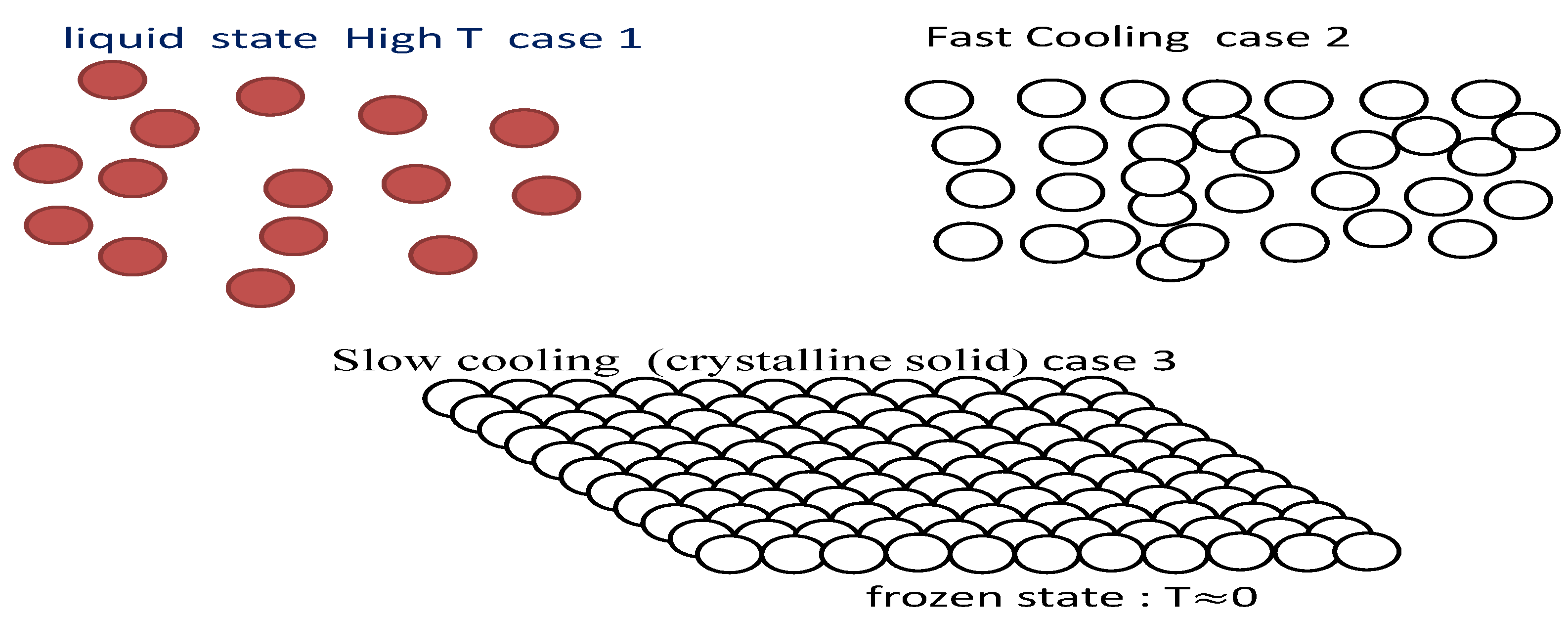
• Decrease carefully the temperature of the solid to reach a ground state (minimal energy state, crystalline structure.

The physical matter in the heat bath has two phases: (1) the solid state at the beginning of the process and (2) the liquid state when the temperature of the heat bath is sufficiently high. In this case, all particles of the solid arrange themselves randomly. In the ground state, the particles are arranged in a highly structured lattice and the energy of the system is minimal. The ground state of the solid is obtained only if the maximum temperature is sufficiently high and the cooling is sufficiently slow. Otherwise, the solid will be frozen into a metastable state rather than into the ground state. We can imagine this physical process (thermodynamic) in Figure 1 and the curve of states in Figure 2. From those phases, we can conclude the following:

∘

In case 1, the matter is in its liquid state, where T is sufficiently high;

∘

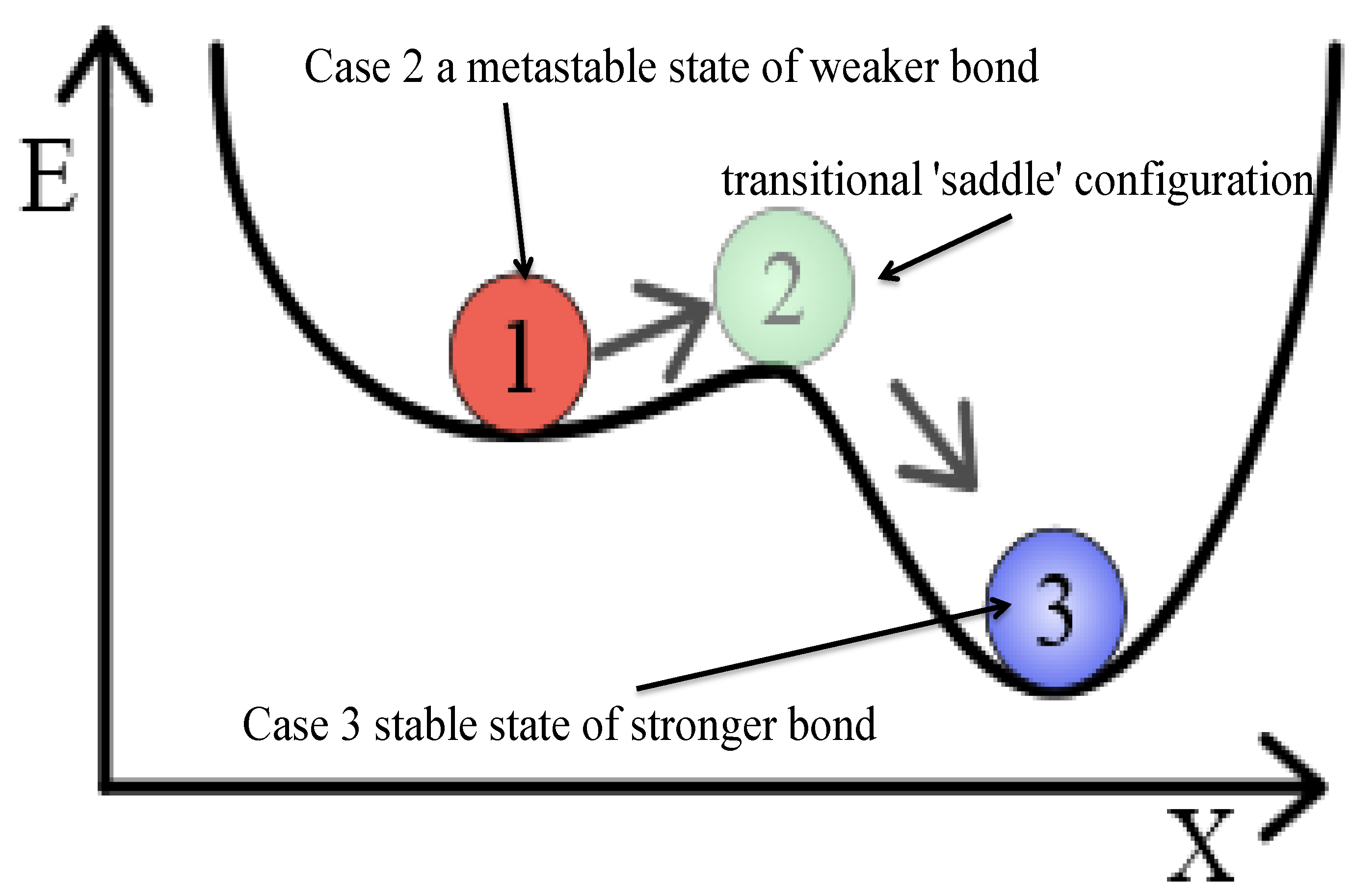
In case 2, the liquid will be frozen into a metastable state (in physics, metastability is a stable state of a dynamical system other than the system’s state of least energy [57]) (converts to a meta-stable state of weaker bond “at fast cooling”);

∘

In case 3, the liquid will be frozen into the ground state (the ground state of a quantum mechanical system is its lowest-energy state; the energy of the ground state is known as the zero-point energy of the system [58]) (at slow cooling).

The detailed description of the simulated-annealing algorithm can be found in [30,38,59].

2.2. Improving the Performance of SA

The simulated annealing algorithm is inspired from the physical annealing. It is also a stochastic method to avoid getting stuck in a local, non-global minima. The simulated annealing is a local search algorithm capable of escaping local optima.

The simulated-annealing algorithm is one of the most successful meta-heuristic computational algorithms, which have been initially designed for discrete optimization especially in the field of combinatorial optimization problems [33]. The SA has also been extended to optimization problems for continuous variables [31]. The fundamental idea of the SA is to allow moves resulting in solutions of worse quality than the current solution (uphill moves) in order to escape from local minima. The probability of such a move is decreased during the search. The basic SA algorithm is listed in Algorithm 1. There are many researchers interested in using the simulated annealing algorithm.

Most authors who deal with improving the SA algorithm considered improving one or more of the following five issues: generation of points, cooling schedule, acceptance criteria, stopping criteria, and inner and outer loops. The authors of [30,31,46] presented various modifications and suggestions to improve the performance of the SA. In this paper, we improve the SA algorithm even farther by considering all of the above five issues. This is the topic of the next section.

3. Proposed Method

As mentioned above, our modifications and suggestions to improve the performance of the simulated annealing algorithm contain five issues. The generation of a candidate solution, acceptance criteria, stopping criterion, and inner loop and outer loop are common points of all algorithms that seek to solve Problem (1). While the cooling schedule is one of the important standards that characterize the simulated annealing algorithms. However, we have made the generation of a candidate solution, acceptance criteria, stopping criterion, and inner loop and outer loop depend on the cooling schedule, as we will see in the next sections, which discuss the five issues.

3.1. Research Direction and a Step Length

The generation of a new point and a best direction are considered as a one of the most important phases of the simulated-annealing algorithm. See [30,31,46] for various suggestions to determine a direction and step length. In the next two subsections, we discuss two approaches to generate a direction and step length along the direction.

In the remaining parts of this section, the notation $x_{ac}$ denotes the best point accepted so far with its value $f_{ac}=f\left(x_{ac}\right)$. At $k=1$, we set $x_{ac}=x_0$, where $x_0$ is the starting point.

3.1.1. First Approach

The first approach is to generate a research direction and step size randomly as follows. They are described in Algorithm 2.

Algorithm 2 First approach for generating a direction and step length

Step 1: Generate a random vector $V\in {[-1,1]}^n.$ Step 2: Set $V_d=\pm 1$, if $V_{{}_i}<0$, $V_d=-1$, otherwise $V_d=1$. Step 3: Generate a random number $p\in (-0.5,0.5).$ Step 4: Compute $g=0.5-p$. Step 5: Compute $dg=g·V_d$. Step 6: Compute $C=\frac{|f_{ac}|}{{\Vert dg\Vert }_2^2}$. Step 7: Compute $d=C·V_d$.

In Step 1 of Algorithm 2, $V\in {[-1,1]}^n$ is a random vector of n dimensions. In Step 2, $V_d=sign\left(V\right)$ is a vector of either 1 or −1. It represents a direction. In Step 3, $p\in (-0.5,0.5)$ is a random number. In Step 5, since g and $V_d$ are both random, then $dg$ is a random vector. In Step 6, we compute C as a step size of $V_d$. In Step 7, d is the step along the direction $V_d$.

We compute a new point by setting:

$$x_1=x_{ac}+d.$$

(2)

After computing $x_1$, we compute $f_1=f\left(x_1\right)$. We now compute $▵f$. If $▵f<0$, then the point $x_1$ is accepted and we set $x_{ac}\leftarrow x_1$, $f_{ac}\leftarrow f_1$. Otherwise, we generate another point by the second approach as in Section 3.1.2 below. We note the following.

Note 1: The above-mentioned processes are repeated at each iteration k, with $k=1,2,\dots ,M$, where M denotes the inner loop maximum number of iterations and its value is set in advance.

Note 2: We set $x_g=x_{ac}$ as the global minimum, when the outer criterion is satisfied as we will see later in Section 3.5.

3.1.2. Second Approach

This approach is similar to the approach suggested in [30,31,46,60], with some major modifications. We specify a step length ${\delta }_i$ and a direction $d{v}_i$ of this step. Let us first state Algorithm 3.

Algorithm 3 Second approach to generate a direction and step length

Step 1: Set $i=0$. Step 2: Compute ${\mu }_i={10}^{(0.1·i)}$ Step 3: Generate a random vector $v_i\in {[-1,1]}^n$. Step 4: Compute $d_i^j=\frac{{(1+{\mu }_i)}^{\mid v_i^j\mid }-1}{{\mu }_i}$, where $j=1,2,\dots ,n$. Step 5: Set $d{v}_i^j=\pm 1$, if $v_i^j<0$, $d{v}_i^j=-1$, otherwise $d{v}_i^j=1$. Step 6: Compute $d{e}_i^j=d_i^j·d{v}_i^j$. Step 7: Compute ${\delta }_i^j=b_j·d{e}_i^j$. Step 8: $i\leftarrow i+1$. Step 9: Repeat steps 2–8 until $i=N$.

In Algorithm 3, N is the maximum number of possible trials and is set in advance. The parameter $v_{{}_i}$ is a random vector having a uniform distribution $U[-1,1]$, b is the upper bound of the domain search and n is the dimension of x. In Step 5, $d{v}_{{}_i}^j$ is the jth component of the vector $d{v}_{{}_i}$. In general, the superscript j denotes the jth component of a vector. Thus, $v_i^j$ is the jth component of the vector $v_{{}_i}$. In Step 7, we multiply $d{e}_{{}_i}$ by b to ensure that the vector ${\delta }_{{}_i}$ does not approach zero quickly in order to obtain the best point.

We compute a new point by using the following equation:

$$x_{2_{{}_i}}=x_{ac}+{\delta }_{{}_i}.$$

(3)

The new point $x_{2_{{}_i}}$ is obtained by adding the point $x_{ac}$ as the best point accepted so far to ${\delta }_i$, at a number of trials i. For example, at $i=1$, the processes in Algorithm 3, give $d{v}_{{}_1}$ as a direction, ${\delta }_{{}_1}$ is a step length, a point $x_{2_{{}_1}}$ is computed as a new point using Equation (3). The value $f_2=f\left(x_{2_{{}_1}}\right)$ is computed. We now compute $▵f=f_2-f_{ac}$. The point $x_{2_{{}_1}}$ is tested for acceptance. Steps 2–8 in Algorithm 3 are repeated until $i=N$. At every iteration i, we obtain a candidate point $x_{2_i}$. The points are either accepted or rejected according to the Metropolis et al. [32] criteria as we will show in Section 3.2 below. In this case, if the point $x_{2_i}$ is rejected, we generate another point randomly as follows.

$$x_{2_{{}_i}}=\{\begin{array}{ll}{x}_{2_{{}_{i-1}}}+{\beta }_i& \mathrm{if} x_{2_{{}_{i-1}}} \mathrm{in} \left(3\right) \mathrm{is} \mathrm{accepted}, \mathrm{i.e.}, i\ge 2\\ {\beta }_i& \mathrm{otherwise}, \mathrm{i.e.}, i\ge 1,\end{array}$$

(4)

where ${\beta }_{{}_i}$ is a random vector ${\beta }_{{}_i}\in {(0,1)}^n$. After N trials, we obtain a succession of candidate points $x_{2_{{}_0}}$, $x_{2_{{}_1}}$,…, $x_{2_{{}_i}}$,…, $x_{2_{{}_N}}$. They are computed by Equations (3) or (4).

Note 1: The point $x_{2_{{}_i}}$ is generated by Equation (4) if the point in Equation (3) is not accepted so far.

Note 2: If the point $x_{2_{{}_i}}$ in Equation (3) is accepted at least once, then the next point is generated either using Equation (3) or Equation (4). As we will see in Section 3.2.

Note 3: The interior-point technique is used when a simple bounded ${[a;b]}^n$ exists in the test problem to ensure that the new point lies inside ${[a;b]}^n$.

3.2. Acceptance of Steps

In our proposed method, we start with any point $x_0$, set $x_{ac}=x_0$ and compute $f_{ac}$. A point $x_1$ is generated using Equation (2). Compute the value $\Delta f=f_1-f_{ac}$, if $\Delta f<0$, then the point $x_1$ is accepted and set $x_{ac}\leftarrow x_1$, $f_{ac}\leftarrow f_1$. Otherwise, we have two cases to generate another point $x_{2_i}$ as follows:

Case 1: We generate a point $x_{2_i}$ using Equation (3) and compute the value $\Delta f=f_{2_{{}_i}}-f_{ac}$ if $\Delta f<0$ or $r<e^{\frac{-▵f}{T}}$, where $r\in (0,1)$ is a random number, then we accept the point $x_{2_{{}_i}}$ and set $x_{a{c}_{{}_i}}\leftarrow x_{2_{{}_i}}$, $f_{a{c}_{{}_i}}\leftarrow f\left(x_{2_{{}_{{}_i}}}\right)$.

Case 2: If the point $x_{2_i}$ in case 1 is rejected, we generate another point $x_{2_{{}_i}}$ by using Formula (4). and directly accept it.

Now, we set $x_{a{c}_{{}_i}}\leftarrow x_{2_i}$, $f_{a{c}_{{}_i}}\leftarrow f\left(x_{2_{{}_i}}\right)$.

As a summary of the above two cases, we obtain a new point denoted by $x_{a{c}_{{}_i}}$, as an accepted point according to the following:

$$x_{{\mathrm{ac}}_{{}_i}}=\{\begin{array}{ll}{x}_{2_{{}_i}}& \mathrm{in}(3); \mathrm{if} ▵f<0 \mathrm{or} r<e^{\frac{-▵f}{T}},\\ x_{2_{{}_i}}& \mathrm{in} (4);\mathrm{if}{x}_{2_{{}_{i-1}}}\mathrm{in} (3) \mathrm{is} \mathrm{accepted}, \mathrm{i.e.}, i\ge 1\\ x_{2_{{}_i}}& \mathrm{in} \left(4\right);\mathrm{otherwise}, \mathrm{i.e.}, i\ge 0,\end{array}$$

(5)

where the first branch of Equation (5) is the acceptance criteria of Metropolis in [32]. The second branch of Equation (5) is applied if a point in Equation (3) is rejected after acceptance. Therefore, we obtained a sequence of accepted points $x_{a{c}_{{}_1}}$, $x_{a{c}_{{}_2}}$,…, $x_{a{c}_{{}_i}}$,…, $x_{a{c}_{{}_N}}$. We pick the best of them, $x_{best}$, as the point that gives the best optimal value of f and set $x_{ac}\leftarrow x_{best}$, $f_{ac}\leftarrow f\left(x_{best}\right)$. This scenario is shown by Figure 3 and Algorithm 4.

Algorithm 4 Efficient Modified Meta-Heuristic Technique “EMST”

Input : $f:{\mathbb{R}}^n\to \mathbb{R}$, $x_0\in {\mathbb{R}}^n$, M, N, T, $T_{f1}$, $T_{f2}$, $\epsilon >0$ Output : $x_{{}_{{}_g}}=x_{{}_{ac}}$ the global minimizer of f, $f(x_{{}_{{}_g}})$, the value of f at $x_{{}_{{}_g}}$. 1: Compute $f\left(x_0\right)$. 2: Set $x_{ac}=x_0$, $f_{ac}=f\left(x_0\right)$, $f_b=f\left(x_0\right)$, and $\lambda =1$.                                  ▹. 3: while $(T>T_{f1}$ and $\lambda >\epsilon )$ or $(T>T_{f2})$ do 4:     for $k=0$ to M do 5:         Compute $x_k=x_{ac}+d$, as in Equation (2). 6:         Compute $f\left(x_k\right)$ and set $▵f=f\left(x_k\right)-f_{ac}$. 7:         if $▵f<0$ then 8:            $x_{ac}\leftarrow x_k$ and $f_{ac}\leftarrow f\left(x_k\right)$. 9:         else 10:            for $i=0$ to N do 11:                Compute $x_{2_{{}_i}}=x_{ac}+{\delta }_i$ as in Equation (3). 12:                Compute $f(x_{2_{{}_i}})$ and $▵f=f(x_{2_{{}_i}})-f_{ac}$. 13:                if $▵f<0$ then 14:                    Accept=True. 15:                else if $r<e^{-\frac{▵f}{T}}$ then 16:                    Accept=True. 17:                else 18:                    Compute $x_{2_i}$, by using Formula (4). 19:                    Compute $f\left(x_{2_i}\right)$. 20:                    Accept=True. 21:                end if 22:                if $Accept==True$ then 23:                    $x_{a{c}_{{}_i}}\leftarrow x_{2_{{}_i}}$ and $f_{a{c}_{{}_i}}\leftarrow f\left(x_{2_{{}_i}}\right)$. 24:                    Store accepted points with their values in the matrix $A_{i\times (n+1)}=[x_{a{c}_{{}_i}}:f_{a{c}_{{}_i}}]$. 25:                end if 26:            end for 27:            Sort $A_{N\times (n+1)}$ with respect to $f_{ac}$ we get the minimum value $f_{best}$ at a point $x_{best}$. 28:            Set $x_{ac}\leftarrow x_{best}$, $f_{ac}\leftarrow f_{best}$. 29:         end if 30:         Store accepted points with their function values in the matrix $B_{k\times (n+1)}=[x_{ac}:f_{ac}]$. 31:     end for 32:     Sort $B_{M\times (n+1)}$ with respect to $f_{ac}$ we get the minimum value $f_{best}$ at a point $x_{best}$. 33:     Set $x_{ac}\leftarrow x_{best}$, $f_{ac}\leftarrow f_{best}$. 34:     Set $f_a\leftarrow f_{ac}$. 35:     Compute $\lambda =|f_b-f_a|$. 36:     $f_b\leftarrow f_a$. 37:     Decrease temperature $T=r_T\ast T$. 38: end while 39: Set $x_g\leftarrow x_{ac}$, $f_g\leftarrow f_{ac}$. 40: return $x_g$ the global minimizer and the value of function at $x_g$, $f\left(x_g\right)$.

3.3. Cooling Schedule

The choice of a cooling scheduling has an important impact on the performance of the simulated-annealing algorithm. The cooling schedule includes two terms: the initial value of the temperature T and the cooling coefficient $r_T$, which is used to reduce T. Many suggestions have been proposed in the literature for determining the initial value of the temperature T and the cooling coefficient $r_T$, see, for example, [30,31,46,49].

In general, it is a unanimous fact that the initial temperature T must be sufficiently high and $r_T\in (0.1,1)$. In this section, we suggest that the initial value of T be related to the number of variables and the value of $f\left(x\right)$ at the starting point $x_0$. See Section 4.1. The cooling coefficient is taken to be $r_T\in [0.8,1)$ to decrease the temperature T slowly.

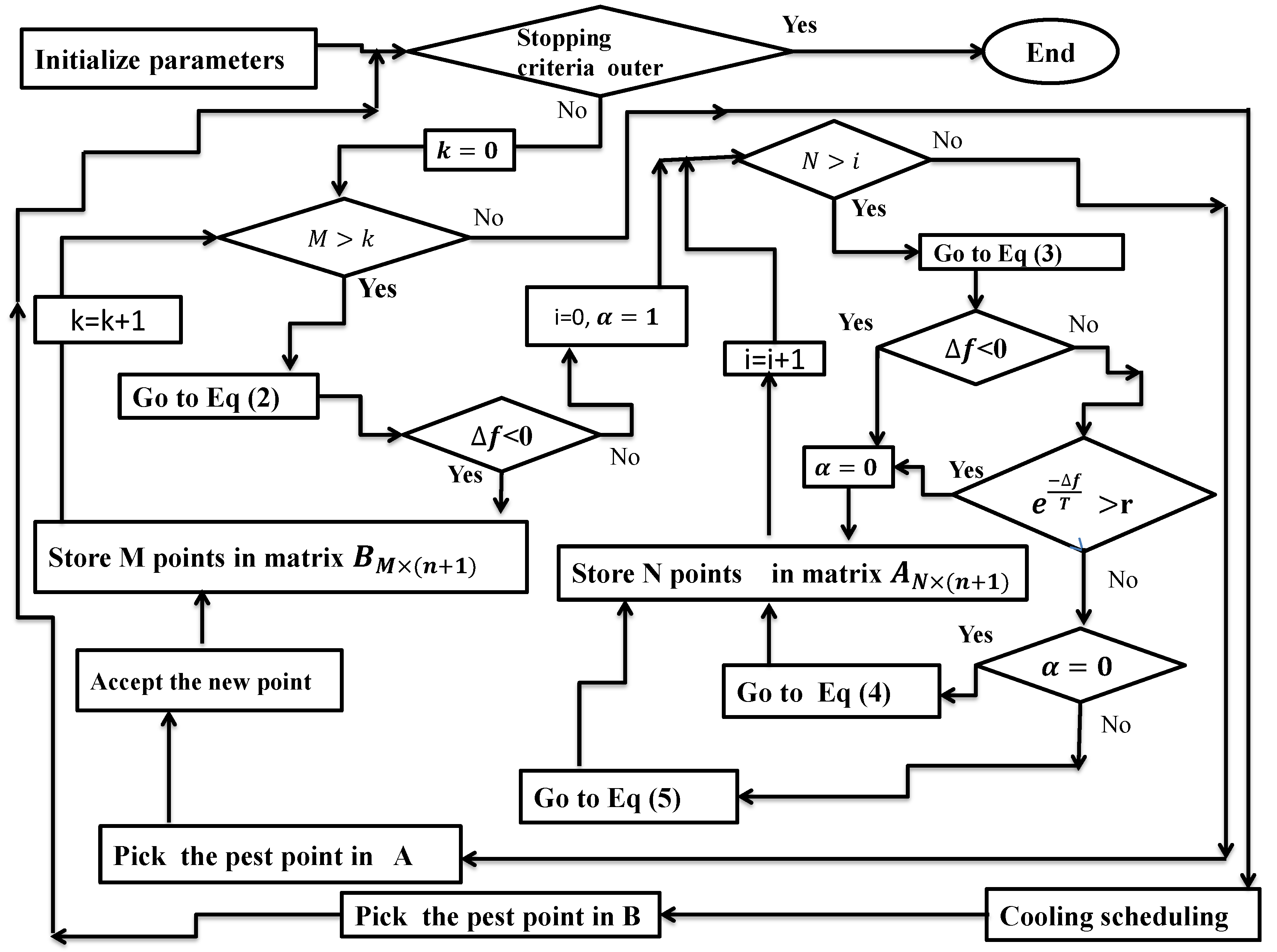
3.4. Algorithm’s Loops

The loop iterations is presented in different formats in the literature, see, for example, [30,31,41,44,46].

In this section, we suggest three loop iterations for the whole process of the proposed method. They are as follows.

• The outer loop, which reduces the temperature T.
• The inner loop, which has a finite number of iterations. Particularly from 1 to M, where M is a preconceived maximum number of iterations.
• In the second approach, we generate N trials to obtain N points at each iteration k.

3.5. Stopping Criteria

To terminate the simulated-annealing algorithm, several stopping rules are given in the literature. See, for example, [30,31,46]. Almost all stopping criteria presented in the literature are based on the idea that the algorithm should be terminated, when the system freezes (i.e., $T\to 0$) and no further changes occur.

In this proposed algorithm, the stopping criteria considered are as follows:

• Outer loop stopping criterion: the algorithm will be terminated if one of the following is satisfied: Either $(T<T_{f1}$ and $\lambda =0)$ or $(T<T_{f2})$, where $\lambda =|f_b-f_a|$, $f_a$ denotes a value of function at a best point after “M” iterations as inner loop iterations, $f_b$ denotes a value of function at the starting point. The value of $\lambda$ is computed, we set $f_b\leftarrow f_a$, $T_{f2}$ and $T_{f1}$ are sufficiently small with ($T_{f2}<T_{f1}$).
• Inner loop stopping criterion: this loop continues until it reaches a pre-specified maximum number of inner iterations denoted by M.

The overall algorithm is presented below. It contains all suggestions and modifications that are presented in Section 3.1–Section 3.5 to obtain the new proposed algorithm. We call it “Efficient Modified Meta-heuristic Technique”, abbreviated by “EMST”.

4. Numerical Experiments

To test the efficiency of the proposed Algorithm “EMST”, we solved thirty-one test problems. The functions in the test problems have different convexity shapes. The results show that the new algorithm is promising.

4.1. Setting Parameters

The parameters $T_{f1}$ and $T_{f2}$, are introduced in Section 3.5. In our numerical testing, we set the follows values for $T_{f1}$.

$$T_{f1}=\left\{\begin{array}{cc}{10}^{-4}\hfill & \mathrm{if}n<4\hfill \\ {10}^{-10}\hfill & \mathrm{if}n<10\mathrm{and} |f_0|<100n\hfill \\ {10}^{-6}\hfill & \mathrm{otherwise},\hfill \end{array}\right.$$

where $|f_0|$ denotes the absolute value of the function at the starting point $x_0$, and n is the number of variables. The parameter $T_{f2}$ takes the values:

$$T_{f2}=\left\{\begin{array}{cc}{10}^{-6}\hfill & \mathrm{if}n<4\hfill \\ {10}^{-15}\hfill & \mathrm{if}n<10\mathrm{and} |f_0|<100n\hfill \\ {10}^{-10}\hfill & \mathrm{otherwise}.\hfill \end{array}\right.$$

The parameter M in the inner loop is taken to be:

$$M=\left\{\begin{array}{cc}3n\hfill & \mathrm{if}n<4\hfill \\ 2n\hfill & \mathrm{if}4\le n\le 10\hfill \\ 10n\hfill & \mathrm{otherwise}.\hfill \end{array}\right.$$

For the parameter T, we take $T=100n+|f_0|$ as a starting value for the temperature.

The parameter $r_T$ is the cooling coefficient. It is taken to be:

$$r_T=\left\{\begin{array}{cc}0.8\hfill & \mathrm{if}T>200n\hfill \\ 0.95\hfill & \mathrm{if}{T}_{new}>10n\hfill \\ 0.8\hfill & \mathrm{otherwise}.\hfill \end{array}\right.$$

For all test problems with parameter T, that satisfies $T>200n$, the parameter $r_T$ will be 0.8 for each iteration k (until the outer criteria are satisfied). Otherwise, the parameter $r_T$ will be 0.95, until the condition $T_{new}<10n$ is satisfied. After that, $r_T$ will be 0.8, until the outer criteria are satisfied.

We update the temperature by using $T_{new}=T_{new}\ast r_T$. However, at the beginning, we take $T_{new}=T$. The parameter N denotes the maximum number of iterations needed by Algorithm 3 to generate a new step, see Section 3.1.2. We let N take the values:

$$N=\left\{\begin{array}{cc}80\hfill & \mathrm{if}n<10\mathrm{and} |f_0|<100n\hfill \\ 40n\hfill & \mathrm{if}n\le 10\mathrm{and} |f_0|>100n\hfill \\ 400\hfill & \mathrm{otherwise}.\hfill \end{array}\right.$$

Note: the parameters proposed above have different values due to the difficultly of some problems. Some problems of high dimension require many iterations to reach the optimality.

4.2. Testing Efficiency of Algorithm

We use the same criteria used by the authors of [41,61,62] because we compare the results of our algorithm against the results obtained by the algorithms given in [41,61,62]. The criteria are as follows.

(1)

The rate of success “RS”, which represents the rate of success for trials leading to the global minimum of a problem.

(2)

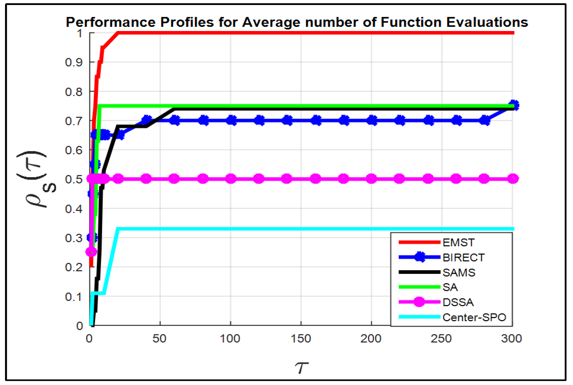
The average number of function evaluations “AFE”.

(3)

The quality of the final result (average error) “AE”.

We use the definition of average error as given in [41,61,62]. It is defined to be:

$$|f\left(x^{*}\right)-f_g|\le {\epsilon }_{{}_1}\left|f\left(x^{*}\right)\right|+{\epsilon }_{{}_2},$$

(6)

where $f\left(x^{*}\right)$ is the exact global minimum and $f_g$ is the best function value obtained by the methods.

A run is considered successful if Inequality (6) is met, where ${\epsilon }_{{}_1}={10}^{-8}$ and ${\epsilon }_{{}_1}={10}^{-6}$.

4.3. Results

All experiments were run on a PC with Intel(R) Core(TM) i5-3230M CPU@2.60 GHz 2.60 GHz with RAM 4.00GB of memory on Windows 10 operating system, all six algorithms are programmed using MATLAB version 8.5.0.197613 (R2015a) and the machine epsilon is about ${10}^{-16}$.

In

Table 2. Listing of different algorithms used in the comparisons.

$\mathit{No}$	Algorithm Name	Algorithm	Reference
1	Global Optimization and Simulated Annealing	“SA”	[31]
2	Direct Search Simulated Annealing	DSSA	[15]
3	Enhancing PSO Methods for Global Optimization	“Center-PSO”	[63]
4	Simulated Annealing Driven multi-Start	“SAMS”	[46]
5	A new DIRECT type Algorithm	BIRECT	[64]
6	Efficient Modified Stochastic Technique	“EMST”	This work

, we present the algorithms that will be used in the comparisons. Column 2 presents the name of the algorithms, Column 3 gives the abbreviated names.

In

Table 3. Listing of test problems and their exact solutions.

f	n	$\mathit{f}\left({\mathit{x}}^{*}\right)$	Reference	f	n	$\mathit{f}\left({\mathit{x}}^{*}\right)$	Reference
$BR$	2	0.397887	[31,63]	$P22$	2	24776.51	[31]
$ES$	2	−1	[61,62,63,65]	$RA$	10	0	[65]
$GP$	2	3	[31,41,61,62,65]	$P8$	3	0	[31]
$Ras$	2	−2	[63]	$CB$	2	−1.0316285	[63,65]
$SH$	2	−186.7309	[31,61,62,65]	$CV$	4	0	[65]
$H3$	3	−3.86278	[31,41,61,62,63,65]	$DJ$	3	0	[61,62]
$S5$	4	−10.1532	[31,41,61,62,63,65,66]	$Bh1$	2	0	[65]
$S7$	4	−10.4029	[31,41,61,62,63,65,66]	$P16$	5	0	[31]
$S10$	4	−10.5364	[31,41,61,62,63,65,66]	$GW$	6,10	0	[65]
$H6$	6	−3.32237	[31,41,61,62,63,65]	$Bh2$	2	0	[65]
$DX10$	10	0	[65]	$PWQ$	4	0	[65]
$R_n$	2–10	0	[61,62,65]	$Tr10$	10	0	[65]
$CM$	4	0.4	[65]	$MGP$	2	1.29695	[65]
$Ack$	10	0	[65]

, we present the test problems used to test the performance of our algorithm. Columns 1, 2 and 3 give the data of the problems. Column 1 represents the name of the function f, Column 2 gives the number of variables n, Column 3 gives the exact global solution of the problem $f\left(x^{*}\right)$ and Column 4 gives the reference in which it appears. Columns 1–4 are repeated in Columns 5–8.

Note: The mathematical expressions of the corresponding test functions can be found in References given in Table 3.

The final results which are obtained by Algorithm 4 are listed in

Table 4. Results of the proposed “EMST” Algorithm.

f	$\mathit{AE}$	$\mathit{AFE}$	f	$\mathit{AE}$	$\mathit{AFE}$	f	$\mathit{AE}$	$\mathit{AFE}$
$BR$	3.6 $\times {10}^{-7}$	456	$P22$	7.3 $\times {10}^{-12}$	541	$ES$	1.1 $\times {10}^{-16}$	501
$GP$	1.1 $\times {10}^{-14}$	456	$RA10$	0	13,232	$Ras$	0	506
$CB$	4.6 $\times {10}^{-8}$	456	$SH$	6.8 $\times {10}^{-6}$	506	$DJ$	2.5 $\times {10}^{-14}$	736
$P8$	6.9 $\times {10}^{-14}$	729	$H3$	2.1 $\times {10}^{-6}$	722	$CV$	4 $\times {10}^{-9}$	6700
$S5$	1.4 $\times {10}^{-6}$	1486	$S7$	3.9 $\times {10}^{-5}$	1486	$S10$	9.6 $\times {10}^{-6}$	1486
$P16$	1.3 $\times {10}^{-9}$	1838	$H6$	1.68 $\times {10}^{-5}$	2172	$GW$	0	13,636
$DX10$	4.1 $\times {10}^{-23}$	11,100	$R_2$	1.21 $\times {10}^{-7}$	456	$R_4$	2.26 $\times {10}^{-5}$	6288
$R_5$	2.56 $\times {10}^{-5}$	8133	$R_8$	9.48 $\times {10}^{-7}$	13,771	$R_{10}$	1.0 $\times {10}^{-6}$	16,756
$Bh1$	1.36 $\times {10}^{-12}$	426	$Bh2$	7.7 $\times {10}^{-13}$	430	$Tr10$	2.53 $\times {10}^{-12}$	10,976
$PWQ4$	2.86 $\times {10}^{-9}$	5609	$Ack$	2.58 $\times {10}^{-14}$	13,030	$CM$	2.4 $\times {10}^{-10}$	1495
$MGP$	4.05 $\times {10}^{-6}$	501

. Column 1 of Table 4 gives the name of the function which is denoted by f. Column 2 of Table 4 gives the average of the error (the accuracy of the solution) that is denoted by $AE$. Column 3 of Table 4 gives the average of the number of the function evaluation that is denoted by $AFE$. Columns 4–9 are as Columns 1–3.

In the following section, the performance profiles of the six algorithms are presented.

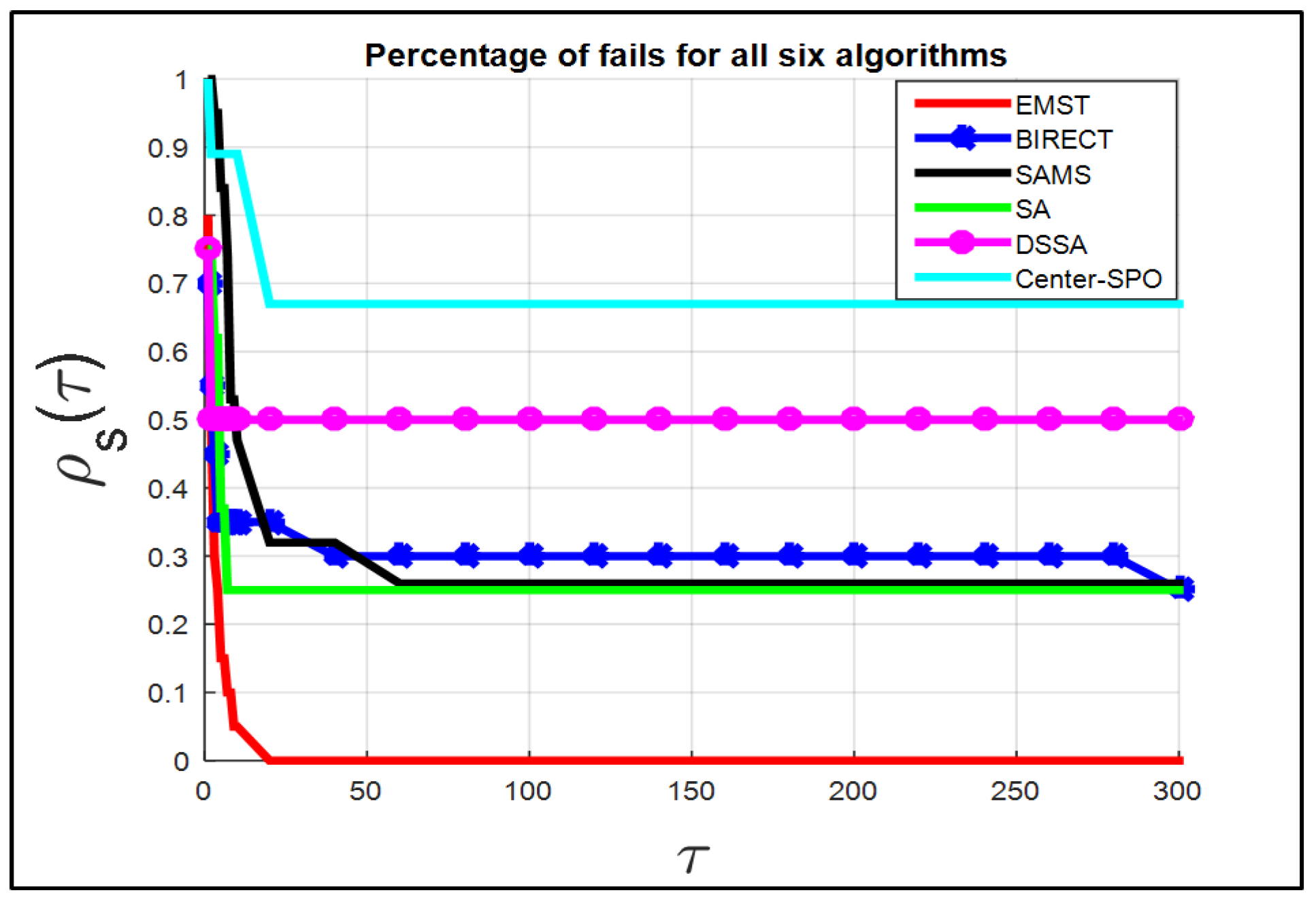
4.4. Performance Profiles

Performance profiles are an important tool used to evaluate and compare the performance of optimization algorithms [67,68,69,70].

Barbosa et al. [67] apply performance profiles to analyze the results of the 2006 CEC constrained optimization competition.

A fair comparison among different solvers should be based on the number of function evaluations, instead of based on the number of iterations or on the CPU time. The number of iterations is not a reliable measure because the amount of work in each iteration is completely different among solvers since some are population-based and other are single-point-based since the quality of the solution is also an important measure of performance [69,70].

In this paper, therefore, the average of function emulations is used to compare the performance of the six algorithms. Hence, we present the numerical results in the form of performance profiles, as described in [68]. This procedure was developed for benchmark optimization software, i.e., to compare different solvers on several test problems.

One advantage of the performance profiles is that they can be presented in one figure, by plotting for the different solvers a cumulative distribution function ${\rho }_{{}_s}\left(\tau \right)$.

The performance ratio is defined by first setting $r_{p,s}=\frac{t_{p,s}}{min\{t_{p,s}:s\in S\}}$, where $p\in P$, P is a set of test problems, S is the set of solvers and $t_{p,s}$ is the value obtained by solver s on test problem p.

Then, define ${\rho }_{{}_s}\left(\tau \right)=\frac{1}{\left|P\right|}\mathrm{size}\{p\in P:r_{p,s}\le \tau \}$, where $\left|P\right|$ is the number of test problems.

In the following, we show how the performance profiles are used to compare the performance of the six algorithms $S=\{EMST,BIRECT,SAMS,Center-spo,DSSA,SA\}$, according to the average function emulations, which is denoted by AEFs.

Therefore, the term $t_{p,s}$ denotes the ${\mathrm{AFE}}_{p,s}$, $\left|P\right|$ is the number of test problems. For each problem p and solver s, the performance ratio is defined as:

$$r_{p,s}=\left\{\begin{array}{cc}\frac{{\mathrm{fit}}_{p,s}}{min\{{\mathrm{AFE}}_{p,s}:s\in S\}}\hfill & \mathrm{if}\mathrm{convergence}\mathrm{test}\mathrm{passed},\hfill \\ \infty \hfill & \mathrm{otherwise},\hfill \end{array}\right.$$

(7)

where ${\mathrm{AFE}}_{p,s}$ represents the function evaluations for the test problem p, which is obtained by the solver s.

Note: Formula (7) means that if the final result $f\left(x^{*}\right)$, obtained by a solver $s\in S$ satisfies Inequality (6), then the first branch of (7) is computed, otherwise, we set $r_{p,s}=\infty$.

The performance profile of a solver s is defined as follows:

$$\delta (r_{p,s},\tau )=\left\{\begin{array}{cc}1\hfill & \mathrm{if}{r}_{p,s}\le \tau ,\hfill \\ 0\hfill & \mathrm{otherwise}.\hfill \end{array}\right.$$

(8)

Therefore, the performance profile for solver s is then given by the following function:

$${\displaystyle {\rho }_{{}_s}\left(\tau \right)=\frac{1}{\left|P\right|}\left\{\sum _{p\in P}\delta (r_{p,s},\tau )\right\},\tau \ge 1.}$$

(9)

By definition of ${\mathrm{AFE}}_{p,s}$, ${\rho }_{{}_s}\left(1\right)$ denotes the fraction of test problems for which solver s performs the best, ${\rho }_{{}_s}\left(2\right)$ gives the fraction of problems for which the solver’s performance is within a factor of two of the best, and that for $\tau$ sufficiently large, ${\rho }_{{}_s}\left(\tau \right)$ is the fraction of problems solved by s. In general, ${\rho }_{{}_s}\left(\tau \right)$ can be interpreted as the probability for solver $s\in S$ that the performance ratio $r_{p,s}$ is within a factor $\tau$ of the best possible ratio. Therefore, ${\rho }_{{}_s}\left(1\right)$ measures the efficiency of the solver, while its robustness (high probability of success on the set P) is measured in terms of ${\rho }_{{}_s}(\infty )$. Hence, if we are only interested in determining which solver is the best, i.e., wins the most, we compare the values of ${\rho }_{{}_s}\left(1\right)$ for all solvers.

A core feature of performance profiles is that they give information on the relative performance of many solvers [68,69].

In the following, the results of the six algorithms are annualized by showing the performance profiles for each algorithm.

Performance Analysis of Algorithms Using Performance Files

Figure 4 shows the performance profiles of the set solvers (algorithms) S regarding the average of function evaluations. The performance of each algorithm depends on the value of parameter $\tau$, we can distinguish the following cases of the values of the $\tau$ to find out how superior each algorithm is.

Case 1:$\tau \in [1,20]$, EMST solves 20–95% of test problems, BIRECT solves 30–65% of test problems, SA solves 25–75% of test problems, SAMS solves 0–68% of test problems, DSSA solves 25–50% of test problems and Center-spo solves 0–11% of test problems. In this case, the three algorithms EMST, BIRECT and SA are the best. However, the proposed algorithm EMST is slightly superior to the BIRECT and SA algorithms.

Case 2:$\tau \in [21,40]$, EMST solves all test problems, BIRECT solves $70\%$ of test problems, SA solves $75\%$ of test problems, SAMS solves 68–74% of problems, DSSA solves $50\%$ of test problems and Center-spo solves $33\%$ of problems. In this case, the three algorithms EMST, SA and SAMS are the best algorithms. However, the proposed algorithm EMST is capable of solving all test problems.

In general, for any value of the parameter $\tau >40$, the EMST algorithm can solve all test problems with less cost compared to other algorithms. Figure 5 shows the percentage of fails of all six algorithms according to the function evaluations.

5. Concluding Remark

We have presented an efficient modified stochastic technique. The computational experiments show the efficiency of the proposed algorithm, for finding the global minima. The suggested “EMST” Algorithm finds the global minimum at each run for all test problems, even though some of the proposed methods in the literature were unable to find the global minima of some test problems at each run.

Combining this suggested stochastic technique “EMST” with classical optimization methods, such as direct search methods, indirect search methods or even with other meta-heuristics methods will improve the performance of the “EMST” algorithm on many problems.

In other words, it is possible to minimize the number of function evaluations by combining (in a hybrid way) the proposed “EMST” algorithm with another inexpensive traditional method. This is a research topic that should be considered.

We think it is possible to extend the proposed method to deal with constrained optimization problems. This is the topic of our future work. Convergence analysis of the “EMST” algorithm will be considered in future work by using homogeneous or inhomogeneous Markov chain theory.

In principle, all meta-heuristic strategies depend on the stochastic search for the next solution. Consequently, the current version of the simulated-annealing algorithm is distinguished from the other algorithms mentioned in this study by the following: the five modified and proposed standard features have granted the new suggested algorithm consecutive opportunities to escape from a local point at each run during finding the global minimizer of the non-convex function. Therefore, this novelty in the proposed algorithm makes it capable of finding the global minimizer of the non-convex function at each run compared to the algorithms that are listed in this study.

References

1. Abdel-Baset, M.; Hezam, I. A Hybrid Flower Pollination Algorithm for Engineering Optimization Problems. Int. J. Comput. Appl. 2016, 140, 10–23. [Google Scholar] [CrossRef]
2. Agrawal, P.; Ganesh, T.; Mohamed, A.W. A novel binary gaining–sharing knowledge-based optimization algorithm for feature selection. Neural Comput. Appl. 2021, 33, 5989–6008. [Google Scholar] [CrossRef]
3. Ayumi, V.; Rere, L.; Fanany, M.I.; Arymurthy, A.M. Optimization of Convolutional Neural Network using Microcanonical Annealing Algorithm. arXiv 2016, arXiv:1610.02306. [Google Scholar]
4. Lobato, F.S.; Steffen, V., Jr. Fish swarm optimization algorithm applied to engineering system design. Lat. Am. J. Solids Struct. 2014, 11, 143–156. [Google Scholar] [CrossRef]
5. Mazhoud, I.; Hadj-Hamou, K.; Bigeon, J.; Joyeux, P. Particle swarm optimization for solving engineering problems: A new constraint-handling mechanism. Eng. Appl. Artif. Intell. 2013, 26, 1263–1273. [Google Scholar] [CrossRef]
6. Mohamed, A.W.; Sabry, H.Z. Constrained optimization based on modified differential evolution algorithm. Inf. Sci. 2012, 194, 171–208. [Google Scholar] [CrossRef]
7. Mohamed, A.W.; Hadi, A.A.; Mohamed, A.K. Gaining-sharing knowledge based algorithm for solving optimization problems: A novel nature-inspired algorithm. Int. J. Mach. Learn. Cybern. 2020, 11, 1501–1529. [Google Scholar] [CrossRef]
8. Rere, L.; Fanany, M.I.; Arymurthy, A.M. Metaheuristic Algorithms for Convolution Neural Network. Comput. Intell. Neurosci. 2016, 2016. [Google Scholar] [CrossRef]
9. Samora, I.; Franca, M.J.; Schleiss, A.J.; Ramos, H.M. Simulated annealing in optimization of energy production in a water supply network. WAter Resour. Manag. 2016, 30, 1533–1547. [Google Scholar] [CrossRef]
10. Shao, Y. Dynamics of an Impulsive Stochastic Predator–Prey System with the Beddington–DeAngelis Functional Response. Axioms 2021, 10, 323. [Google Scholar] [CrossRef]
11. Vallepuga-Espinosa, J.; Cifuentes-Rodríguez, J.; Gutiérrez-Posada, V.; Ubero-Martínez, I. Thermomechanical Optimization of Three-Dimensional Low Heat Generation Microelectronic Packaging Using the Boundary Element Method. Mathematics 2022, 10, 1913. [Google Scholar] [CrossRef]
12. Dennis, J.E., Jr.; Schnabel, R.B. Numerical Methods for Unconstrained Optimization and Nonlinear Equations; Society for Industrial and Applied Mathematics: Philadelphia, PA, USA, 1996; Volume 16. [Google Scholar]
13. Andrei, N. An unconstrained optimization test functions collection. Adv. Model. Optim 2008, 10, 147–161. [Google Scholar]
14. Fan, S.K.S.; Zahara, E. A hybrid simplex search and particle swarm optimization for unconstrained optimization. Eur. J. Oper. Res. 2007, 181, 527–548. [Google Scholar] [CrossRef]
15. Hedar, A.R.; Fukushima, M. Hybrid simulated annealing and direct search method for nonlinear unconstrained global optimization. Optim. Methods Softw. 2002, 17, 891–912. [Google Scholar] [CrossRef]
16. Parouha, R.P.; Verma, P. An innovative hybrid algorithm for bound-unconstrained optimization problems and applications. J. Intell. Manuf. 2022, 33, 1273–1336. [Google Scholar] [CrossRef]
17. Wu, J.Y. Solving unconstrained global optimization problems via hybrid swarm intelligence approaches. Math. Probl. Eng. 2013, 2013. [Google Scholar] [CrossRef]
18. Blum, C.; Roli, A. Metaheuristics in combinatorial optimization: Overview and conceptual comparison. ACM Comput. Surv. (CSUR) 2003, 35, 268–308. [Google Scholar] [CrossRef]
19. Nocedal, J.; Wright, S. Numerical Optimization; Springer Science & Business Media: Berlin, Germany, 2006. [Google Scholar]
20. Aarts, E.; Korst, J. Simulated Annealing and Boltzmann Machines: A Stochastic Approach to Combinatorial Optimization and Neural Computing; John Wiley & Sons, Inc.: New York, NY, USA, 1989. [Google Scholar]
21. Hillier, F.S.; Price, C.C. International Series in Operations Research &amp; Management Science; Springer: Berlin, Germany, 2001. [Google Scholar]
22. Laarhoven, P.J.V.; Aarts, E.H. Simulated Annealing: Theory and Applications; Springer-Science ++ Business Media, B.V.: Berlin, Germany, 1987. [Google Scholar]
23. Kan, A.R.; Timmer, G. Stochastic methods for global optimization. Am. J. Math. Manag. Sci. 1984, 4, 7–40. [Google Scholar] [CrossRef]
24. Ali, M. Some Modified Stochastic Global Optimization Algorithms with Applications. Ph.D. Thesis, University of the Witwatersrand, Johannesburg, South Africa, 1994. [Google Scholar]
25. Desale, S.; Rasool, A.; Andhale, S.; Rane, P. Heuristic and meta-heuristic algorithms and their relevance to the real world: A survey. Int. J. Comp. Eng. Res. Trends 2015, 2, 296–304. [Google Scholar]
26. Alshamrani, A.M.; Alrasheedi, A.F.; Alnowibet, K.A.; Mahdi, S.; Mohamed, A.W. A Hybrid Stochastic Deterministic Algorithm for Solving Unconstrained Optimization Problems. Mathematics 2022, 10, 3032. [Google Scholar] [CrossRef]
27. Chakraborti, S.; Sanyal, S. An Elitist Simulated Annealing Algorithm for Solving Multi Objective Optimization Problems in Internet of Things Design. Int. J. Adv. Netw. Appl. 2015, 7, 2784. [Google Scholar]
28. Gonzales, G.V.; dos Santos, E.D.; Emmendorfer, L.R.; Isoldi, L.A.; Rocha, L.A.O.; Estrada, E.d.S.D. A Comparative Study of Simulated Annealing with different Cooling Schedules for Geometric Optimization of a Heat Transfer Problem According to Constructal Design. Sci. Plena 2015, 11. [Google Scholar] [CrossRef]
29. Poorjafari, V.; Yue, W.L.; Holyoak, N. A Comparison between Genetic Algorithms and Simulated Annealing for Minimizing Transfer Waiting Time in Transit Systems. Int. J. Eng. Technol. 2016, 8, 216. [Google Scholar] [CrossRef]
30. Corona, A.; Marchesi, M.; Martini, C.; Ridella, S. Minimizing multimodal functions of continuous variables with the simulated annealing algorithm. ACM Trans. Math. Softw. 1987, 13, 262–280. [Google Scholar] [CrossRef]
31. Dekkers, A.; Aarts, E. Global optimization and simulated annealing. Math. Program. 1991, 50, 367–393. [Google Scholar] [CrossRef]
32. Metropolis, N.; Rosenbluth, A.W.; Rosenbluth, M.N.; Teller, A.H.; Teller, E. Equation of state calculations by fast computer machines. J. Chem. Phys 1953, 21, 1087–1092. [Google Scholar] [CrossRef]
33. Kirkpatrick, S.; Gelatt, C.D.; Vecchi, M.P. Optimization by simulated annealing. Science 1983, 220, 671–680. [Google Scholar] [CrossRef]
34. Vanderbilt, D.; Louie, S.G. A Monte Carlo simulated-annealing algorithm approach to optimization over continuous variables. J. Comput. Phys. 1984, 56, 259–271. [Google Scholar] [CrossRef]
35. Bohachevsky, I.O.; Johnson, M.E.; Stein, M.L. Generalized simulated annealing for function optimization. Technometrics 1986, 28, 209–217. [Google Scholar] [CrossRef]
36. Anily, S.; Federgruen, A. Simulated annealing methods with general acceptance probabilities. J. Appl. Probab. 1987, 24, 657–667. [Google Scholar] [CrossRef]
37. Ingber, L. Simulated Annealing: Practice versus Theory. Mathl. Comput. Model. 1993, 18, 29–57. [Google Scholar] [CrossRef]
38. Bertsimas, D.; Tsitsiklis, J. Simulated annealing. Stat. Sci. 1993, 8, 10–15. [Google Scholar] [CrossRef]
39. Goffe, W.L.; Ferrier, G.D.; Rogers, J. Global optimization of statistical functions with simulated-annealing algorithm. J. Econom. 1994, 60, 65–99. [Google Scholar] [CrossRef]
40. Tsallis, C.; Stariolo, D.A. Generalized Simulated Annealing. Physica A 1996, 233, 395–406. [Google Scholar] [CrossRef] [Green Version]
41. Siarry, P.; Berthiau, G.; Durbin, F.; Haussy, J. Enhanced Simulated-Annealing Algorithm for Globally Minimizing Functions of Many Continuous Variables. ACM Trans. Math. Softw. 1997, 23, 209–228. [Google Scholar] [CrossRef]
42. Nouraniy, Y.; Andresenz, B. A comparison of simulated-annealing algorithm cooling strategies. J. Phys. A Math. Gen 1998, 31, 8373–8385. [Google Scholar] [CrossRef]
43. Yang, S.; Machado, J.M.; Ni, G.; Ho, S.L.; Zhou, P. A self-learning simulated-annealing for global optimizations of electromagnetic devices. IEEE Trans. Magn. 2000, 36, 1004–1008. [Google Scholar]
44. Ali, M.M.; Torn, A.; Viitanen, S. A direct search variant of the simulated-annealing for optimization involving continuous variables. Comput. Oper. Res. 2002, 29, 87–102. [Google Scholar] [CrossRef]
45. Bouleimen, K.; Lecocq, H. A new efficient simulated annealing algorithm for the resource-constrained project scheduling problem and its multiple mode version. Eur. J. Oper. Res. 2003, 149, 268–281. [Google Scholar] [CrossRef]
46. Ali, M.M.; Gabere, M. A simulated annealing driven multi-start algorithm for bound constrained global optimization. J. Comput. Appl. Math. 2010, 233, 2661–2674. [Google Scholar] [CrossRef]
47. Wang, G.G.; Guo, L.; Gandomi, A.H.; Alavi, A.H.; Duan, H. Simulated annealing-based krill herd algorithm for global optimization. In Proceedings of the Abstract and Applied Analysis; Hindawi Publishing Corporation, Hindawi: London, UK, 2013; Volume 2013. [Google Scholar]
48. Rere, L.R.; Fanany, M.I.; Arymurthy, A.M. Simulated annealing algorithm for deep learning. Procedia Comput. Sci. 2015, 72, 137–144. [Google Scholar] [CrossRef]
49. Certa, A.; Lupo, T.; Passannanti, G. A New Innovative Cooling Law for Simulated Annealing Algorithms. Am. J. Appl. Sci. 2015, 12, 370. [Google Scholar] [CrossRef]
50. Xu, P.; Sui, S.; Du, Z. Application of Hybrid Genetic Algorithm Based on Simulated Annealing in Function Optimization. World Acad. Sci. Eng. Technol. Int. J. Math. Comput. Phys. Electr. Comput. Eng. 2015, 9, 677–680. [Google Scholar]
51. Guodong, Z.; Ying, Z.; Liya, S. Simulated Annealing Optimization Bat Algorithm in Service Migration Joining the Gauss Perturbation. Int. J. Hybrid Inf. Technol. 2015, 8, 47–62. [Google Scholar] [CrossRef]
52. Sirisumrannukul, S. Network reconfiguration for reliability worth enhancement in distribution system by simulated annealing. In Simulated Annealing, Theory with Applications; InTech Open: London, UK, 2010; pp. 161–180. [Google Scholar] [CrossRef]
53. Fradkin, E. Field Theories of Condensed Matter Physics; Cambridge University Press: Cambridge, UK, 2013. [Google Scholar]
54. Downarowicz, T. Entropy structure. J. d’Analyse Math. 2005, 96, 57–116. [Google Scholar] [CrossRef]
55. Lieb, E.H.; Yngvason, J. The physics and mathematics of the second law of thermodynamics. Phys. Rep. 1999, 310, 1–96. [Google Scholar] [CrossRef]
56. Makarov, I. Dynamical entropy for Markov operators. J. Dyn. Control. Syst. 2000, 6, 1–11. [Google Scholar] [CrossRef]
57. Debenedetti, P.G. Metastable Liquids: Concepts and Principles; Princeton University Press: Princeton, NJ, USA, 1996. [Google Scholar]
58. Contributors, W. Metastability. 2018. [Google Scholar]
59. Boussaïd, I.; Lepagnot, J.; Siarry, P. A survey on optimization metaheuristics. Inf. Sci. 2013, 237, 82–117. [Google Scholar] [CrossRef]
60. Yang, W.Y.; Cao, W.; Chung, T.S.; Morris, J. Applied Numerical Methods Using MATLAB; Wiley: Hoboken, NJ, USA, 2005. [Google Scholar]
61. Bessaou, M.; Siarry, P. A genetic algorithm with real-value coding to optimize multimodal continuous functions. Struct. Multidisc Optim. 2001, 23, 63–74. [Google Scholar] [CrossRef]
62. Chelouah, R.; Siarry, P. Tabu search applied to global optimization. Eur. J. Oper. Res. 2000, 123, 256–270. [Google Scholar] [CrossRef]
63. Tsoulos, I.G.; Stavrakoudis, A. Enhancing PSO methods for global optimization. Appl. Math. Comput. 2010, 216, 2988–3001. [Google Scholar] [CrossRef]
64. Paulavičius, R.; Chiter, L.; Žilinskas, J. Global optimization based on bisection of rectangles, function values at diagonals, and a set of Lipschitz constants. J. Glob. Optim. 2018, 71, 5–20. [Google Scholar] [CrossRef]
65. Ali, M.M.; Khompatraporn, C.; Zabinsky, Z.B. A numerical evaluation of several stochastic algorithms on selected continuous global optimization test problems. J. Glob. Optim. 2005, 31, 635–672. [Google Scholar] [CrossRef]
66. Khalil, A.M.; Fateen, S.E.K.; Bonilla-Petriciolet, A. MAKHA-A New Hybrid Swarm Intelligence Global Optimization Algorithm. Algorithms 2015, 8, 336–365. [Google Scholar] [CrossRef]
67. Barbosa, H.J.; Bernardino, H.S.; Barreto, A.M. Using performance profiles to analyze the results of the 2006 CEC constrained optimization competition. In Proceedings of the IEEE Congress on Evolutionary Computation, Barcelona, Spain, 18–23 July 2010; pp. 1–8. [Google Scholar]
68. Dolan, E.D.; Moré, J.J. Benchmarking optimization software with performance profiles. Math. Program. 2002, 91, 201–213. [Google Scholar] [CrossRef]
69. Moré, J.J.; Wild, S.M. Benchmarking derivative-free optimization algorithms. SIAM J. Optim. 2009, 20, 172–191. [Google Scholar] [CrossRef]
70. Vaz, A.I.F.; Vicente, L.N. A particle swarm pattern search method for bound constrained global optimization. J. Glob. Optim. 2007, 39, 197–219. [Google Scholar] [CrossRef] [Green Version]
Figure 1. The cooling phases of solid material.
Axioms 11 00483 g001
Figure 2. Representation of the ground state and the meta-stable state in Figure 1.
Axioms 11 00483 g002
Figure 3. The framework of the proposed method.
Axioms 11 00483 g003
Figure 4. Performance profiles for an average of function evaluations for six algorithms.
Axioms 11 00483 g004
Figure 5. Performance profile fails for an average of function evaluations for six algorithms.
Axioms 11 00483 g005