
Solving Fractional Volterra–Fredholm Integro-Differential Equations via A** Iteration Method
 , , ,
, , ,
Abstract
:1. Introduction
2. Preliminaries
3. Convergence Analysis
- (1).
- Let and , then we haveHowever,Therefore, does not satisfy condition .
- (2).
- We will now show that is a generalized α-Reich–Suzuki nonexpansive mappings with . We consider the following cases:Case I:Let , thenMoreover,Case II:Let and , we haveAlso,Case III:Let and —we obtainAdditionally,Case IV:Let , we obtain
4. -Stability Result
5. Application to Fractional Volterra–Fredholm Integro-Differential Equations
- (H1)
- Two constants and exist such that for any we haveand
- (H2)
- Two functions exist, the set of all positive functions is continuous on such that
- (H3)
- The functions are continuous.
- (H4)
6. Conclusions
Author Contributions
Funding
Data Availability Statement
Conflicts of Interest
References
- Browder, F.E. Fixed-point theorems for noncompact mappings in Hilbert space. Proc. Natl. Acad. Sci. USA 1965, 53, 1272–1276. [Google Scholar] [CrossRef] [PubMed]
- Browder, F.E. Nonexpansive nonlinear operators in Banach spaces. Proc. Natl. Acad. Sci. USA 1965, 54, 1041–1044. [Google Scholar] [CrossRef] [PubMed]
- Göhde, D. Zum Prinzip def Kontraktiven Abbilding. Math. Nachr. 1965, 30, 251–258. [Google Scholar] [CrossRef]
- Goebel, K.; Kirk, W.A. Iteration processes for nonexpansive mappings. In Topological Methods in Nonlinear Functional Analysis; Singh, S.P., Thomeier, S., Watson, B., Eds.; Contemporary Mathematics; American Mathematical Society: Providence, RI, USA, 1983; Volume 21, pp. 115–123. [Google Scholar]
- Goebel, K.; Kirk, W.A. Topics in Metric Fixed Point Theory; Cambridge University Press: Cambridge, UK, 1990. [Google Scholar]
- Suzuki, T. Fixed point theorems and convergence theorems for some generalized nonexpansive mappings. J. Math. Anal. Appl. 2008, 340, 1088–1095. [Google Scholar] [CrossRef]
- Aoyama, K.; Kohsaka, F. Fixed point theorem for α-nonexpansive mappings in Banach spaces. Nonlinear Anal. 2011, 74, 4387–4391. [Google Scholar] [CrossRef]
- Pant, D.; Shukla, R. Approximating fixed points of generalized α-nonexpansive mappings in Banach spaces. Numer. Funct. Anal. Optim. 2017, 38, 248–266. [Google Scholar] [CrossRef]
- Pant, R.; Pandey, R. Existence and convergence results for a class of non-expansive type mappings in hyperbolic spaces. Appl. Gen. Topol. 2019, 20, 281–295. [Google Scholar] [CrossRef]
- Pandey, R.; Pant, R.; Rakocevic, V.; Shukla, R. Approximating Fixed Points of a General Class of Nonexpansive Mappings in Banach Spaces with Applications. Results Math. 2019, 74, 7. [Google Scholar] [CrossRef]
- Banach, S. Sur les opérations dans les ensembles abstraits et leurs application aux équations intégrales. Fund. Math. 1922, 3, 133–181. [Google Scholar] [CrossRef]
- Hussain, A.; Hussain, N.; Ali, D. Estimation of Newly Established Iterative Scheme for Generalized Nonexpansive Mappings. J. Funct. Space 2021, 2021, 6675979. [Google Scholar] [CrossRef]
- Hussain, A.; Ali, D.; Karapinar, E. Stability data dependency and errors estimation for a general iteration method. Alex. Eng. J. 2021, 60, 703–710. [Google Scholar] [CrossRef]
- Ishikawa, S. Fixed points and iteration of a nonexpansive mapping in a Banach space. Proc. Am. Math. Soc. 1976, 59, 65–71. [Google Scholar] [CrossRef]
- Khan, H.S. A Picard-Man hybrid iterative process. Fixed Point Theory Appl. 2013, 2013, 1–10. [Google Scholar] [CrossRef]
- Noor, M.A. New approximation schemes for general variational inequalities. J. Math. Anal. Appl. 2000, 251, 217–229. [Google Scholar] [CrossRef]
- Ofem, A.E.; Igbokwe, D.I. A new faster four step iterative algorithm for Suzuki generalized nonexpansive mappings with an application. Adv. Theory Nonlinear Anal. Its Appl. 2021, 5, 482–506. [Google Scholar] [CrossRef]
- Ofem, A.E.; Işik, H.; Ali, F.; Ahmad, J. A new iterative approximation scheme for Reich–Suzuki type nonexpansive operators with an application. J. Inequal. Appl. 2022, 2022, 28. [Google Scholar] [CrossRef]
- Ofem, A.E.; Udofia, U.E.; Igbokwe, D.I. A robust iterative approach for solving nonlinear Volterra Delay integro-differential equations. Ural. Math. J. 2021, 7, 59–85. [Google Scholar] [CrossRef]
- Güsoy, F. A Picard-S iterative Scheme for Approximating Fixed Point of Weak-Contraction Mappings. Filomat 2021, 30. [Google Scholar] [CrossRef]
- Mann, W.R. Mean value methods in iteration. Proc. Am. Math. Soc. 1953, 4, 506–510. [Google Scholar] [CrossRef]
- Agarwal, R.P.; O’Regan, D.; Sahu, D.R. Iterative construction of fixed points of nearly asymptotically nonexpansive mappings. J. Nonlinear Convex Anal. 2007, 8, 61–79. [Google Scholar]
- Abbas, M.; Nazir, T. A new faster iteration process applied to constrained minimization and feasibility problems. Mat. Vesnik. 2014, 66, 223–234. [Google Scholar]
- Ullah, K.; Arshad, M. Numerical Reckoning Fixed Points for Suzuki’s Generalized Nonexpansive Mappings via New Iteration Process. Filomat 2018, 32, 187–196. [Google Scholar] [CrossRef] [Green Version]
- Ali, J.; Ali, F. A new iterative scheme to approximating fixed points and the solution of a delay differential equation. J. Nonlinear Convex Anal. 2020, 21, 2151–2163. [Google Scholar]
- Senter, H.F.; Dotson, W.G. Approximating fixed points of nonexpansive mappings. Proc. Am. Math. Soc. 1974, 44, 375–380. [Google Scholar] [CrossRef]
- Schu, J. Weak and strong convergence to fixed points of asymptotically nonexpansive mappings. B. Aust. Math. Soc. 1991, 43, 153–159. [Google Scholar] [CrossRef]
- Berinde, V. On the approximation of fixed points of weak contractive mapping. Carpath. J. Math. 2003, 19, 7–22. [Google Scholar]
- Cardinali, T.; Rubbioni, P. A generalization of the Caristi fixed point theorem in metric spaces. Fixed Point Theory 2010, 11, 3–10. [Google Scholar]
- Timis, I. On the weak stability of Picard iteration for some contractive type mappings. Ann. Univ. Craiova Math. Comput. Sci. Ser. 2010, 37, 106–114. [Google Scholar]
- Marcdanov, M.J.; Sharifov, Y.A.; Aliyev, H.N. Existence and Uniqueness of Solution for Nonlinear Fractional Integro-Differential Equations with Nonlocal Boundary Conditions. Eur. J. Pure Appl. Math. 2022, 15, 726–735. [Google Scholar]
- Ahmad, S.; Ullah, A.; Partohaghighi, M.; Saifullah, S.; Akgul, A.; Jarad, F. Oscillatory and complex behaviour of Caputo-Fabrizio fractional order HIV-1 infection mode. Aims Math. 2022, 7, 4778–4792. [Google Scholar] [CrossRef]
- Rahman, M.; Arfan, M.; Shah, Z.; Alzahran, E. Evolution of fractional mathematical model for drinking under Atangana-Baleanu Caputo derivatives. Phys. Scr. 2021, 96, 115203. [Google Scholar] [CrossRef]
- Rahman, M.; Ahmad, S.; Arfan, M.; Akgul, A.; Jarad, F. Fractional Order Mathematical Model of Serial Killing with Different Choices of Control Strategy. Fractal Fract. 2022, 6, 162. [Google Scholar] [CrossRef]
- Mamoud, A.; Ghadle, K.P.; Isa, M.S.B.; Giniswamy, G. Existence and Uniqueness Theorems for Fractional Volterra-Fredholm Integro-Differential Equations. Int. J. Appl. Math. 2018, 31, 33–348. [Google Scholar]


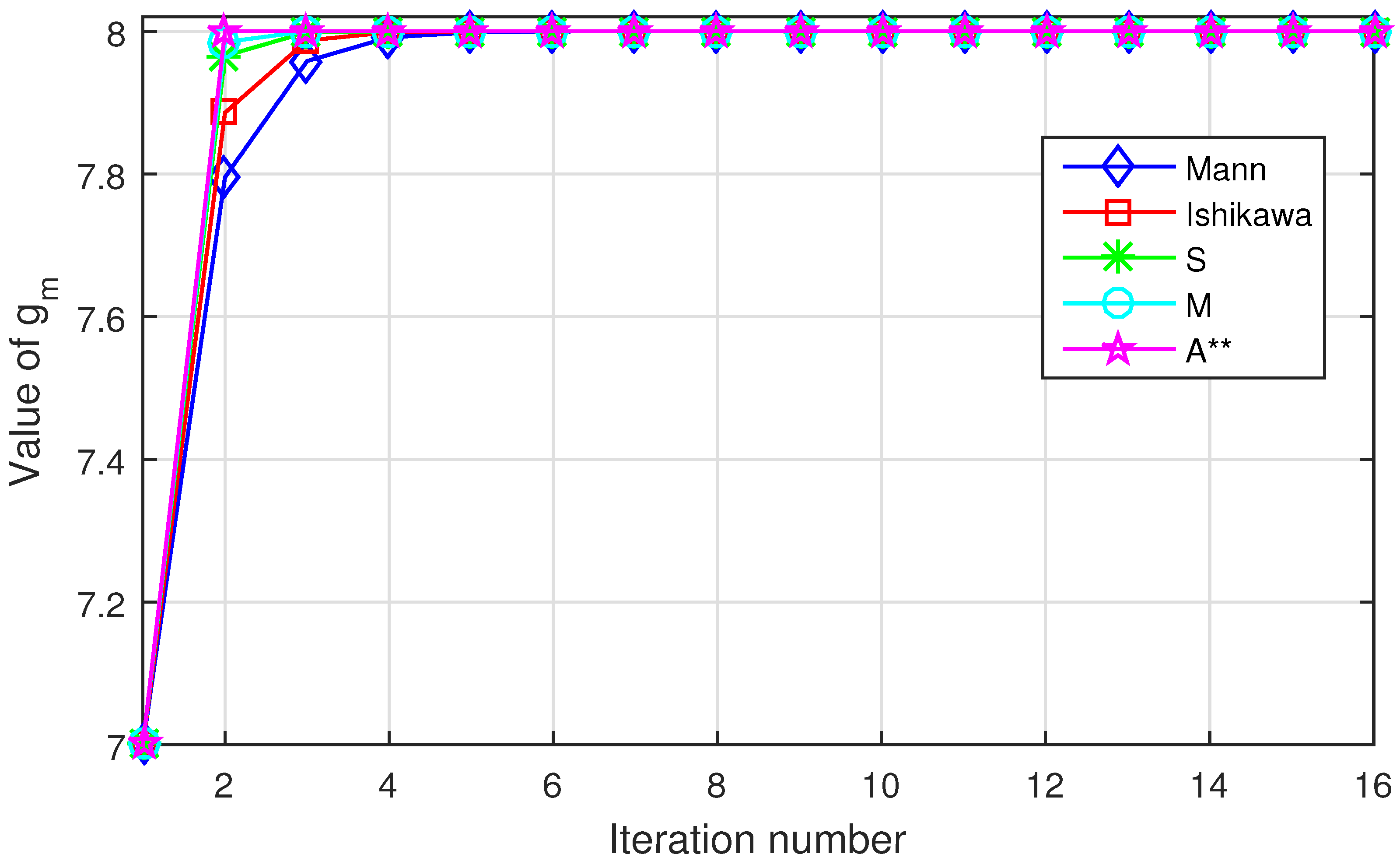
| Mann | Ishikawa | S | M | ||
|---|---|---|---|---|---|
| 7.0000000000 | 7.0000000000 | 7.0000000000 | 7.0000000000 | 7.0000000000 | |
| 7.7954545455 | 7.8858471074 | 7.9653925620 | 7.9968039773 | 7.9999937578 | |
| 7.9581611570 | 7.9869691171 | 7.9988023252 | 7.9999897854 | 8.0000000000 | |
| 7.9914420548 | 7.9985124870 | 7.9999585515 | 7.9999999674 | 8.0000000000 | |
| 7.9982495112 | 7.9998301961 | 7.9999985656 | 7.9999999999 | 8.0000000000 | |
| 7.9996419455 | 7.9999806164 | 7.9999999504 | 8.0000000000 | 8.0000000000 | |
| 7.9999267616 | 7.9999977873 | 7.9999999983 | 8.0000000000 | 8.0000000000 | |
| 7.9999850194 | 7.9999997474 | 7.9999999999 | 8.0000000000 | 8.0000000000 | |
| 7.9999969358 | 7.9999999712 | 8.0000000000 | 8.0000000000 | 8.0000000000 | |
| 7.9999993732 | 7.9999999967 | 8.0000000000 | 8.0000000000 | 8.0000000000 | |
| 7.9999998718 | 7.9999999996 | 8.0000000000 | 8.0000000000 | 8.0000000000 | |
| 7.9999999738 | 8.0000000000 | 8.0000000000 | 8.0000000000 | 8.0000000000 | |
| 7.9999999946 | 8.0000000000 | 8.0000000000 | 8.0000000000 | 8.0000000000 | |
| 7.9999999989 | 8.0000000000 | 8.0000000000 | 8.0000000000 | 8.0000000000 | |
| 7.9999999998 | 8.0000000000 | 8.0000000000 | 8.0000000000 | 8.0000000000 | |
| 8.0000000000 | 8.0000000000 | 8.0000000000 | 8.0000000000 | 8.0000000000 |
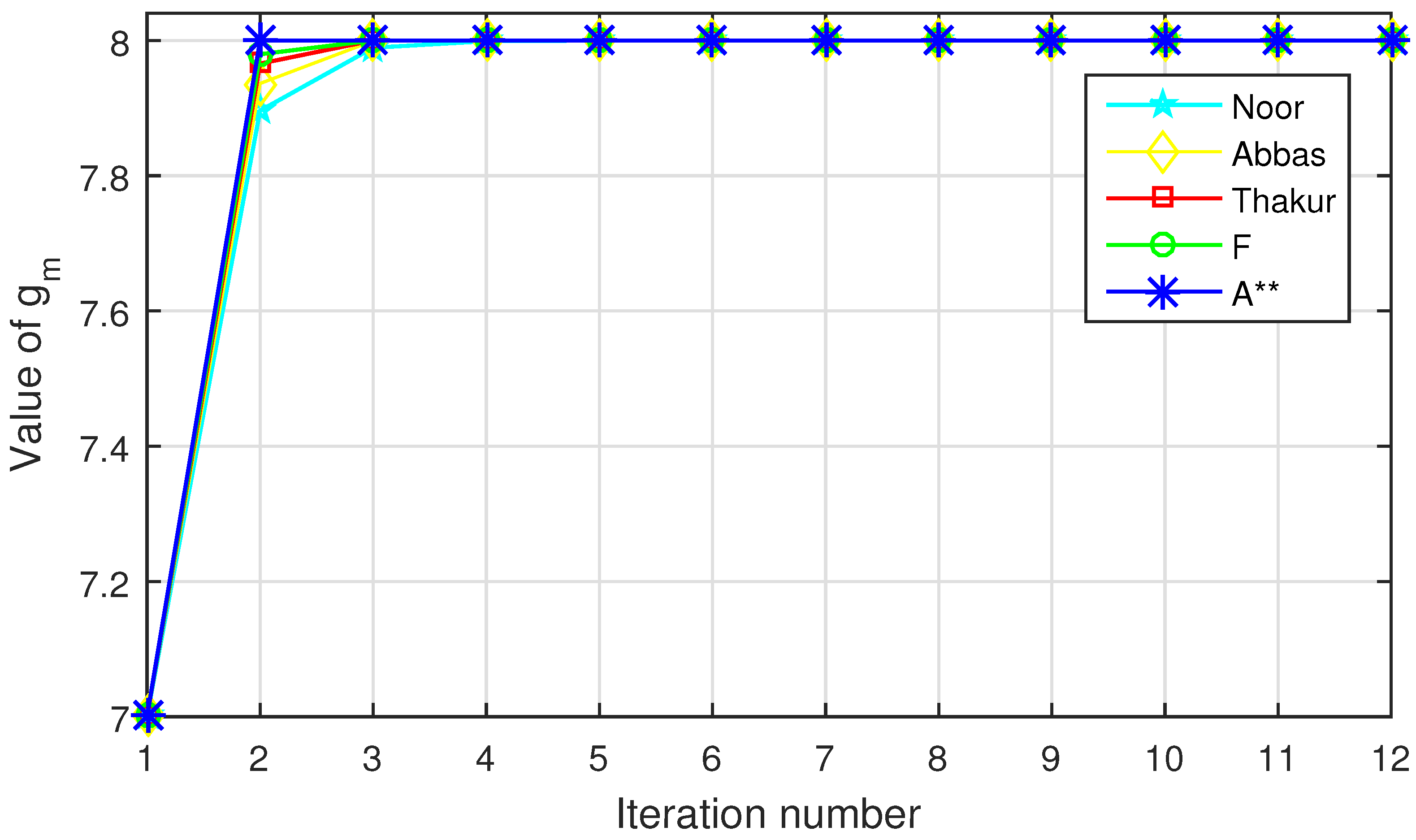
| Noor | Abbas | Thakur | F | ||
|---|---|---|---|---|---|
| 7.0000000000 | 7.0000000000 | 7.0000000000 | 7.0000000000 | 7.0000000000 | |
| 7.8961189895 | 7.9763629320 | 7.9956740702 | 7.9996004972 | 7.9999937578 | |
| 7.9892087357 | 7.9994412890 | 7.9999812863 | 7.9999998404 | 8.0000000000 | |
| 7.9988789926 | 7.9999867937 | 7.9999999190 | 7.9999999999 | 8.0000000000 | |
| 7.9998835486 | 7.9999996878 | 7.9999999996 | 8.0000000000 | 8.0000000000 | |
| 7.9999879029 | 7.9999999926 | 8.0000000000 | 8.0000000000 | 8.0000000000 | |
| 7.9999987433 | 7.9999999998 | 8.0000000000 | 8.0000000000 | 8.0000000000 | |
| 7.9999998695 | 8.0000000000 | 8.0000000000 | 8.0000000000 | 8.0000000000 | |
| 7.9999999864 | 8.0000000000 | 8.0000000000 | 8.0000000000 | 8.0000000000 | |
| 7.9999999986 | 8.0000000000 | 8.0000000000 | 8.0000000000 | 8.0000000000 | |
| 7.9999999999 | 8.0000000000 | 8.0000000000 | 8.0000000000 | 8.0000000000 | |
| 8.0000000000 | 8.0000000000 | 8.0000000000 | 8.0000000000 | 8.0000000000 |
Publisher’s Note: MDPI stays neutral with regard to jurisdictional claims in published maps and institutional affiliations. |
© 2022 by the authors. Licensee MDPI, Basel, Switzerland. This article is an open access article distributed under the terms and conditions of the Creative Commons Attribution (CC BY) license (https://creativecommons.org/licenses/by/4.0/).
Share and Cite
Ofem, A.E.; Hussain, A.; Joseph, O.; Udo, M.O.; Ishtiaq, U.; Al Sulami, H.; Chikwe, C.F. Solving Fractional Volterra–Fredholm Integro-Differential Equations via A** Iteration Method. Axioms 2022, 11, 470. https://doi.org/10.3390/axioms11090470
Ofem AE, Hussain A, Joseph O, Udo MO, Ishtiaq U, Al Sulami H, Chikwe CF. Solving Fractional Volterra–Fredholm Integro-Differential Equations via A** Iteration Method. Axioms. 2022; 11(9):470. https://doi.org/10.3390/axioms11090470
Chicago/Turabian StyleOfem, Austine Efut, Aftab Hussain, Oboyi Joseph, Mfon Okon Udo, Umar Ishtiaq, Hamed Al Sulami, and Chukwuka Fernando Chikwe. 2022. "Solving Fractional Volterra–Fredholm Integro-Differential Equations via A** Iteration Method" Axioms 11, no. 9: 470. https://doi.org/10.3390/axioms11090470