Article

Feature Selection Methods for Extreme Learning Machines

1
School of Automation, Xi’an University of Posts and Telecommunications, Xi’an 710121, China
2
Xi’an Key Laboratory of Advanced Control and Intelligent Process, Xi’an 710121, China
3
School of Computer Science & Technology, Xi’an University of Posts and Telecommunications, Xi’an 710121, China
4
No. 92677 Troops of PLA, Qingdao 266100, China
*
Authors to whom correspondence should be addressed.
Axioms 2022, 11(9), 444; https://doi.org/10.3390/axioms11090444
Submission received: 1 August 2022 / Revised: 14 August 2022 / Accepted: 26 August 2022 / Published: 30 August 2022
(This article belongs to the Special Issue Soft Computing with Applications to Decision Making and Data Mining)

Abstract

:
Extreme learning machines (ELMs) have gained acceptance owing to their high efficiency and outstanding generalization ability. As a key component of data preprocessing, feature selection methods can decrease the noise or irrelevant data for ELMs. However, ELMs still do not have their own practical feature selection method for their special mechanism. In this study, we proposed a feature selection method for the ELM, named FELM. The proposed algorithm achieves highly efficient dimensionality reduction due to the feature ranking strategy. The FELM can simultaneously complete the feature selection and classification processes. In addition, by incorporating a memorization–generalization kernel into the FELM, the nonlinear case of it is issued (called FKELM). The FKELM can achieve high classification accuracy and extensive generalization by applying the property of memorization of training data. According to the experimental results on different artificial and benchmark datasets, the proposed algorithms achieve significantly better classification accuracy and faster training than the other methods.

1. Introduction

Feature selection plays an essential role by removing the irrelevant features and identifying the relevant ones. In 1997, Dash [1] reported on the four parts of a typical feature selection method: generation procedures, evaluation functions, stopping criteria, and verification processes. The feature selection progresses as summarized in the flowchart in Figure 1. First, a subset is extracted from the complete set of features. Then, the feature subset is evaluated by applying an evaluation function. Next, the evaluation result is compared with the stopping criteria. Last, if the evaluation result meets the stopping criteria, the feature selection process stops; otherwise, a new iteration starts by extracting another feature subset. The selected subset of features is generally validated.
Depending on whether they are independent of a learning algorithm, feature selection methods can be divided into four categories: filter [2], hybrid [3], embedded [4], and wrapper methods [5]. Filter methods, such as the fisher [6] and distance [7] scores, are general methods that do not employ any classifier. They can be applied to datasets with a large number of features and require high computing speed. Embedded methods, such as decision tree classification [8], take considerable time interacting with other learning algorithms to complete the feature selection process. Hybrid methods studied in recent years combine the performance of filter and wrapper methods. Wrapper methods are greedy algorithms that depend on classifiers to select or exclude several features based on objective functions [9]. Different classification models can be constructed for different feature subsets, and the merit of these to be considered the best subset is measured by taking the classification performance of selected features as the criterion [10]. Wrapper methods are extensively used in different areas leveraging their high identification accuracy [11].
In 1995, Vapnik proposed an algorithm named support vector machine (SVM), a two-class classifier with maximum interval on the feature space, which can provide the solution to convex quadratic programming problems with good classification performance [12]. A twin support vector machine (TWSVM) comprises two nonparallel hyperplanes four times faster than an SVM [13]. Extreme learning machines (ELMs), first proposed by Huang [14], are learning algorithms for single-hidden-layer feedforward networks (SLFNs) that have attracted significant attention because of their high efficiency and robustness [15]. ELMs randomly generate input bias and weights and obtain outputs by computing the Moore–Penrose generalized inverse matrix H. Nevertheless, according to the results in [16], ELMs have greater generalization ability and higher learning speed than SVMs and TWSVMs.
Various feature selection methods that can accelerate computation and reduce dimensionality have been investigated in many fields. Numerous feature selection methods are based on SVMs and ELMs. These methods have attracted some attention because they can improve the performance of the original classifiers [17]. In 2002, Guyon [18] proposed a wrapper feature selection method based on SVMs, called support vector machine recursive feature elimination, which can reduce the search space and provide a priori knowledge to improve the recognition efficiency and accuracy. Chang [19] achieved good performance by combining linear SVMs with various feature ranking methods. However, these methods are highly complex and can only solve linear problems. Thus, finding an algorithm that is both highly efficient and capable of solving nonlinear problems is crucial. In 2004, Mangasarian presented a new algorithm called the reduced feature support vector machine (RFSVM), which combined a diagonal matrix E with nonlinear SVM classifiers [20]. Similarly, Bai [21] proposed a wrapper feature selection method that added a diagonal matrix E to a TWSVM (FTSVM), effectively identifying the relevant features and improving the performance of the TWSVM. Both used wrapper methods, simultaneously accomplishing the feature selection and classification processes. Man [22] proposed a novel ELM ensemble model that predicts reservoir properties utilizing the nonlinear capability of functional networks to select the optimal input features. In 2014, Adesina formulated an evolutionary wrapper feature selection method using an ELM as the base classifier of a genetic algorithm that explored the space of feature combinations [23]. The feature selection method and the ELM processed the datasets independently. Unlike SVMs, ELMs offer highly accurate and stable classification results at a high learning speed. Therefore, wrapper feature selection methods must be investigated based on ELMs and kernel extreme learning machines (KELMs). Vapnik et al. [24] incorporated a memorization–generalization kernel into an SVM applicable in nonlinear cases. The resulting model exhibited an extensive generalization ability, but it only performed well on datasets with a moderate number of low-dimensional training samples.
This paper makes the following three contributions:
  • A wrapper feature selection method is proposed for the ELM, called FELM. In the FELM, the corresponding objective function and hyperplane are introduced by adding a feature selection matrix, a diagonal matrix with element either 1 or 0 to the objective functions of the ELM. The FELM can effectively reduce the dimensionality of the input space and remove redundant features.
  • The FELM is extended to the nonlinear case (called FKELM) by incorporating a kernel function that combines generalization and memorization radial basis function (RBF) kernels into the FELM. The FKELM can obtain high classification accuracy and extensive generalization by fully applying the property of memorization of training data.
  • A feature ranking strategy is proposed, which can evaluate features based on their contributions to the objective functions of the FELM and FKELM. After obtaining the best matrix E, the resulting methods significantly improve the classification accuracy, generalization performance, and learning speed.
The rest of this study is organized as follows. Section 2 introduces related works, including the ELM and memorization–generalization kernel. In Section 3, the FELM and FKELM are presented. The effectiveness of the proposed algorithms is assessed, and the experimental results, including dimensionality reduction and classification, are dis-cussed in Section 4. Section 5 presents the conclusions of the study and suggests future research directions.

2. Related Works

2.1. ELM

The use of ELMs as SLFNs has gained huge importance in academia and industry [12]. The development of SLFNs has enhanced the generalization performance and speed of ELMs for classification and regression. In ELMs, as long as the hidden layer node of the feedforward nerve is nonlinear phase continuous, the neural network can arbitrarily approach the continuous objective function or classification target without adjusting the hidden layer node. Figure 2 shows the basic structure of ELMs.
In an ELM, for Q random distinct samples x i , t i , x i = x i 1 , x i 2 , , x i m T R m and t i = t i 1 , t i 2 , , t i n T R n , and x i and t i represent the i-th input or actual output vectors, respectively. The relationship between input x i and the expected output f x i is given by:
f x i = j = 1 P β j G ϖ j , b j , x i = j = 1 P β j G ϖ j x i + b j = h x β ,                     i = 1 , 2 , , Q
where ϖ j = ϖ j 1 , ϖ j 2 , , ϖ j n T and b j = b j 1 , b j 2 , , b j n T are the randomly generated learning parameters of the hidden nodes; β j = β j 1 , β j 2 , , β j n T is the vector of weights connecting the hidden layer with the output nodes; h x = h 1 x , , h P x T is the hidden node output for input x R m ; G represents the activation function; and P is the number of hidden nodes. The output function of the ELM can be expressed as:
H β = y
where β = β 1 , β 2 , , β P T is the matrix of output weights and y = y 1 , y 2 , , y Q T is the matrix of targets. The hidden layer output matrix is:
H = G ϖ 1 , b 1 , x 1 G ϖ P , b P , x 1 G ϖ 1 , b 1 , x Q G ϖ P , b P , x Q
When the training error reaches zero, i = 1 N β h x i y i = 0 . The value of the output weights β can be determined by calculating the linear system given by Equation (2):
β = H + y
where H + is the Moore–Penrose generalized inverse matrix [25].
To reduce the possibility of over-fitting the training error should not be equal to zero. When i = 1 N β h x i y i 0 , the objective function of the ELM can be written as:
min       1 2 β 2 + C i = 1 N ξ i s . t .               y i β h x i 1 ξ i   ,       ξ i 0 ,       i = 1 , , N      
where ξ i is the training error of the ith input pattern.

2.2. Memorization–Generalization Kernel

Vapnik et al. [24] proposed a memorization–generalization kernel for SVMs and demonstrated that SVMs using such a kernel could be accomplished with no training errors and display superior performance.
Specifically, the kernel contains both a generalization RBF kernel:
K g x , x ' = exp σ 2 x x ' 2
and a memorization RBF kernel:
K m x , x ' = exp σ 2 x x ' 2
Figure 3a,b show plots of σ σ > 0 , respectively. The memorization–generalization algorithm uses the weighted combination of both kernels, as follows:
K m g x , x ' = 1 τ exp σ 2 x x ' 2 + τ exp σ 2 x x ' 2
where τ (0 ≤ τ ≤ 1) is the weight of the memorization kernel. The combined kernel is shown in Figure 3c. One of these kernels (denoted σ ) is responsible for memorization, while the other one (denoted σ ) is responsible for generalization. When τ = 1 and σ σ > 0 , the kernel only memorizes classification in small areas around the training data point [24].
In this study, we embedded the combined kernel into a feature selection method based on an ELM, significantly improving its classification performance. The resulting FKELM method is described in Section 3 and the experimental results are discussed in Section 4.

3. Proposed Methods

In this section, we describe two novel feature selection algorithms for solving classification problems, namely FELM and FKELM. In addition, the memorization–generalization kernel is first explored within the FELM framework. The weighted kernel combines the benefits of both the generalization and memorization RBF kernels, thereby significantly decreasing the training error of the classifiers and improving the generalization accuracy of the resulting model. The proposed schemes are obtained by solving quadratic programming problems (QPPs). Furthermore, we use a feature ranking method to assess the contributions of the features to the objective functions of ELM and KELM, respectively, achieving a stable performance.

3.1. Mathematical Model

To select features based on an ELM, we introduce a feature selection binary diagonal matrix E and seek one hyperplane:
g x = h x E β = 0
The zeros in the diagonal of E correspond to the suppressed input space features; in contrast, the ones corresponding to the important features effectively utilized in Equation (9), i.e., the feature selection matrix E, defines a subspace spanned by the selected features. The resulting FELM objective function is:
min       1 2 β 2 2 + C e T ξ + ψ e T E e s . t .               h x E β e ξ ,       ξ 0 ,           E = d i a g 0         o r       1
where e is a vector of ones of appropriate dimension, and C > 0 and ψ 0 are parameters used to control the loss ξ = i = 1 N h x i E β y i and the number of selected features (since e T E e = t r a c e E ), respectively. As ψ increases, the penalty on the number of features begins to dominate the objective function.
Before solving Equation (10), we extend it to a nonlinear case, namely FKELM, by seeking a kernel-generated surface corresponding to those in [20] with a feature selection matrix E, as follows:
g x = K m g x E , E x ' β = 0
The modified FKELM objective function is:
min       1 2 K m g x E , E x ' β 2 2 + C e T ξ + ψ e T E e s . t .               K m g x E , E x ' β e ξ ,       ξ 0 ,           E = d i a g 0         o r       1
where C > 0 and ψ 0 are parameters to control the loss ξ = i = 1 N K m g x E , E x ' β y i and number of selected features (since e T E e = t r a c e E ), respectively. As ψ increases, the penalty on the number of features begins to dominate the objective.

3.2. Solutions of FELM and FKELM

Using the feature selection matrix E, the relevant features can be easily determined by solving QPPs. A local solution to Equations (9) and (11) can be obtained by first fixing E and finding the corresponding output weights β , and then fixing the output weights β and going through the components of E, successively updating only those whose modification decreases the objective function.
The Lagrangian functions are as follows:
L β , ξ , ψ , α , λ = 1 2 β 2 2 + C e T ξ + ψ e T E e α T h x E β + ξ e λ T ξ
L β , ξ , ψ , α , λ = 1 2 K m g x E , E x ' β 2 2 + C e T ξ + ψ e T E e α T K m g x E , E x ' β + ξ e λ T ξ
where α = α 1 , α 2 , , α Q T and λ = λ 1 , λ 2 , , λ Q T are the vectors of Lagrange multipliers.
The Karush–Kuhn–Tucker (KKT) conditions for β , ξ , α   and λ in FELM are given by:
β L = β h x E α = 0
ξ L = C e α λ = 0
α T h x E β + ξ e = 0
λ T ξ = 0
α 0 , λ 0
According to Equation (16), 0 λ C is obtained. Therefore, the output weight of FELM is β = h x E α .
Similarly, the KKT conditions for β , ξ , α   and λ in FKELM are given by:
β L = K m g x E , E x ' T K m g x E , E x ' β K m g x E , E x ' α = 0
ξ L = C e α λ = 0
α T K m g x E , E x ' β + ξ e = 0
λ T ξ = 0
α 0 , λ 0
According to Equation (21), 0 λ C is obtained. Thus, the output weight of FKELM is β = K m g x E , E x ' T K m g x E , E x ' - 1 K m g x E , E x ' α .
Before solving the above equations, the feature selection matrix E should be initialized. The strategy of actively initializing E, instead of just assigning random values as in RFSVM and FTSVM, makes the algorithm significantly more stable. Thus, the value of each feature is computed after solving the FELM and FKELM, as follows:
V a l u e F E L M i =   1 2   β 2 2 + C e T e h x β +
V a l u e F K E L M i =   1 2   K m g x i , x ' i β 2 2 + C e T e K m g x i , x ' i β +
where + replaces the negative elements with zeros, and x i refers to the ith column of x. Note that for the selected features, ψ e T E e in Equation (10) and (12) is a constant, and this part is ignored in Equations (25) and (26). The scores of the ith feature that show its importance are computed as follows:
S c o r e F E L M i = V a l u e F E L M i V a l u e F E L M i
S c o r e F K E L M i = V a l u e F K E L M i V a l u e F K E L M i
Consequently, the algorithm progresses as follows. First, an initial E matrix is generated based on the resulting scores, by assigning a value of E i i = 0 if S c o r e i < 1 n , otherwise E i i = 1 . Next, the matrix E is updated by switching the value of each element in the diagonal (from 1 to 0, or from 0 to 1) if the objective function (Equations (10) or (12)) decreases more than the tolerance. Otherwise, the first n elements in the diagonal are changed, until no diagonal element in E can be changed to make the objective function decrease more than the tolerance. Lastly, after updating E, β is recomputed. The algorithm terminates if the objective function decreases less than the tolerance. By repeating this process, input space features can be suppressed. We summarize the proposed FELM and FKELM approaches below.

3.3. Computational Complexity Analysis

The time complexity of the two proposed approaches when solving Equations (10) and (12), including the computation of f E and the repeated execution of step 6, are presented in Algorithms 1 and 2. According to [24], the newly developed methods incorporating a memorization–generalization kernel into the FELM have the same computational complexity as the FELM. Thus, we only discuss the computational complexity of the latter. It is clear that f E is computed no more than k times and β is easy to obtain by calculating the generalized inverse. For matrix H R Q × P , where P is the number of hidden nodes, n is the number of outputs, and Q is the number of datasets, the computational complexity for obtaining the generalized inverse is O P 3 + P 2 Q + P Q n [25]. Compared with RFSVM and FTSVM, FELM and FKELM do not need compute bias b, dramatically reducing the computational time.
Algorithm 1 Feature selection method for ELM
Input: Samples A R m × n ;
      Appropriate parameters C, ψ ;
      A fixed and large integer k, which is the number of sweeps through E;
      Stopping tolerance tol = 1e-6;
Output: Output weight β ;
     E = d i a g 1     o r     0
  1. Set E = I , solve the Equation (10) with the fixed E;
  2. Compute each feature score by Equation (27), for i = 1 , , n , if S c o r e F E L M i < 1 n , then
  set E i i = 0 ;
  3. Solve Equation (10) with the fixed E, and obtain β ;
  4. Repeat
  5. For l = 1 , 2 , , k n and j = 1 + l 1     mod     n :
    (1) Replace E j j from 1 to 0 (or 0 to 1).
    (2) Compute f E = 1 2 β 2 2 + C e T e h x β + + ψ e T E e before and after changing
    E j j .
    (3) Keep the new E j j only if f E decreases more than the tolerance. Else undo the
   change of E j j , and go to (1) if j < n .
    (4) Go to step 6 if the total decrease in f E is less than or equal to tol in the last n
   steps.
  6. Solve the Equation (10) with the new E, and compute β .
  7. Until the objective function decrease of Equation (10) is less than tol if β is changed.
Algorithm 2 Feature selection method for KELM
Input: Samples A R m × n ;
      Appropriate parameters C, ψ ;
      Appropriate parameters in kernel τ , σ , σ ;
      A fixed and large integer k, which is the number of sweeps through E;
      Stopping tolerance tol=1e-6;
Output: Output weight β ;
       E = d i a g 1     o r     0 .
  1. Set E = I , solve the Equation (12) with the fixed E;
  2. Compute each feature score by Equation (28), for i = 1 , , n , if S c o r e F K E L M i < 1 n , then
  set E i i = 0 ;
  3. Solve Equation (12) with the fixed E, and obtain β ;
  4. Repeat
  5. For l = 1 , 2 , , k n and j = 1 + l 1     mod     n :
    (1) Replace E j j from 1 to 0 (or 0 to 1).
    (2) Compute f E = 1 2 K m g x E , E x ' β 2 2 + C e T e K m g x E , E x ' β + + ψ e T E e be-
   fore and after changing E j j .
    (3) Keep the new E j j only if f E decreases more than the tolerance. Else undo the
   change of E j j , and go to (1) if j < n .
    (4) Go to step 6 if the total decrease in f E is less than or equal to tol in the last n
   steps.
  6. Solve the Equation (12) with the new E, and compute β .
  7. Until the Equation (12) is less than tol if β is changed.

4. Experimental Results

We conducted experiments to evaluate the efficiency of the proposed algorithms in dimensionality reduction and classification. Section 4.1 describes classification performance, while Section 4.2 shows qualitative assessment of the different algorithms. For comparison, we also evaluated related algorithms, including the RFSVM and FTSVM, on two artificial datasets and eight benchmark datasets obtained from the UCI machine learning repository [26] and gene datasets [27,28]. All experiments were performed using MATLAB R2016a on a desktop computer with an Intel Core i7–1160G7 CPU at 2.11–GHz, 16 GB of memory, and Windows 10.

4.1. Classification Performance

This section discusses several experiments conducted to verify the classification capacity of the proposed FELM and FKELM methods. We compared their performance with the RFSVM and FTSVM using two artificial and eight real-world datasets collected from the UCI machine learning repository. In the experiments, the FELM and FKELM used the sigmoid function F ( a , b , x ) = 1 1 + exp a i T x + b i as the activation function. The grid search with a cross-validation technique was used to select the optimum parameters [29] C for each dataset, which were, in turn, tuned from 2 10 , , 2 0 , , 2 10 . For each dataset, we evaluated the accuracy and time at ψ = 0 , 2 0 , , 2 4 . Specifically, the memorization–generalization kernel used in FEKLM is given as K m g x , x ' = 1 τ exp σ 2 x x ' 2 + τ exp σ 2 x x ' 2 with kernel parameters τ   ,         σ   ,       σ . According to σ σ > 0 , in this study we set σ = 2 - 10 σ . The parameters τ , σ are selected from 0 , , 0.5 , , 1 and 2 10 , , 2 0 , , 2 10 , respectively. For the RFSVM and FTSVM, the popular Gaussian kernel K x , x i = exp x x i 2 2 σ 2 with parameter σ selected from 2 5 , , 2 0 , , 2 5 is used for the non-linear cases. We select the parameters C 1 = c 11 = c 21 2 8 , , 2 7 and C 2 = c 12 = c 22 2 8 , , 2 7 for the FTSVM [21]. Taking the “two-moon dataset” as an example, we analysed the sensitivity of the FELM and FKELM to the number of hidden layer nodes P. As shown in Figure 4 and Figure 5, as the number of hidden layer nodes increases, the training accuracies of the FKELM and FELM do not exhibit a significant variation. Thus, the optimum number of hidden layer neurons P is set as 300 for all cases. All the datasets are binary class datasets. Therefore, to test the performance of the methods listed above, we defined the accuracy as follows, a c c u r a c y = T P + T N / T P + F P + T N + F N × 100 % , with TP, TN, FP, and FN representing the number of true positive, true negative, false positive, and false negative samples, respectively. The training and test accuracies were taken as the average of 10 experiments.

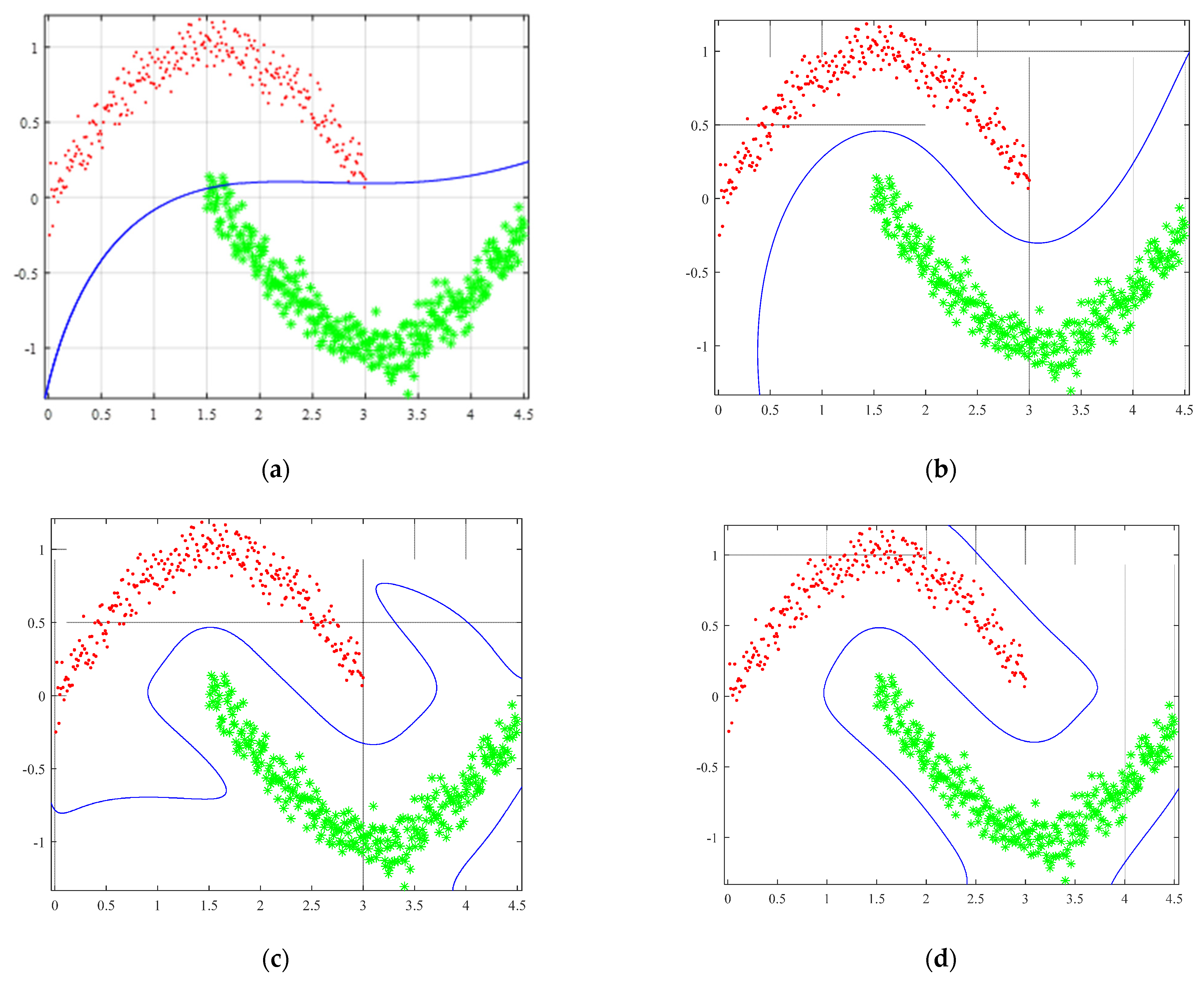
4.1.1. Performance on the Artificial Datasets

Two different artificial datasets were created to graphically depict the classifiers and to verify their accuracy and feature selection ability. All the positive and negative samples on the “two-moon dataset” were completely divided. On the contrary, several positive and negative samples were mixed up in the self-defining function dataset. The details of both datasets used are listed in Table 1 and Table 2. In particular, in the self-defining function dataset, the positive and negative samples had the same covariance but a different centre.
We divided the two-dimensional datasets into categories 1 or -1. Hence, we used the zero-valued contour line to simulate the classification hyperplanes, as plotted in Figure 6 and Figure 7 for the RFSVM and FTSVM as well as the proposed approaches, on the two datasets. Furthermore, the classification accuracies and time of all the methods are presented in Table 3.
The results show that the FKELM and FELM outperform the other algorithms, achieving superior classification performance at a high learning speed. Additionally, it can be seen in Table 3 that the FELM and FKELM have significantly faster and better classification effects than the RFSVM and FTSVM. Because samples are definitely divided, almost all the classifiers obtain high accuracy on the “two-moon dataset”. It is also clear in Figure 7 that the classification hyperplanes obtained from the RFSVM and FTSVM misclassify some positive and negative samples, whereas the proposed FELM and FKELM can correctly divide them into different datasets.

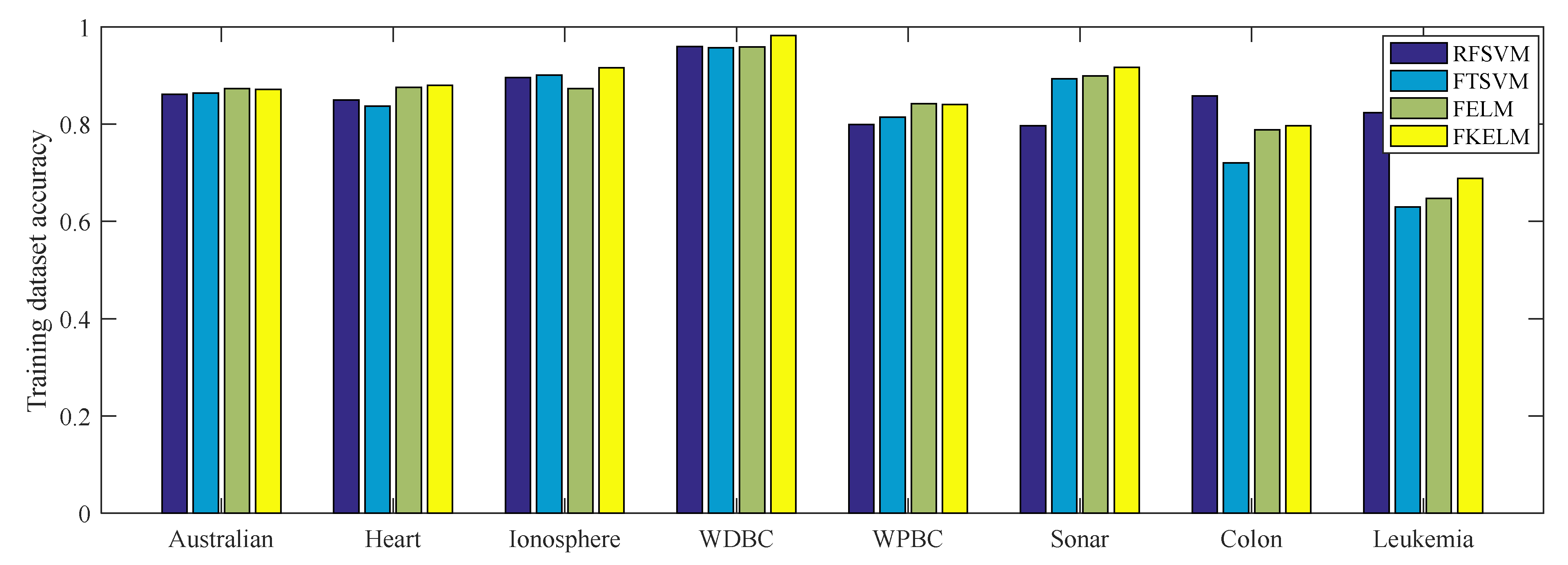
4.1.2. Performance on the Benchmark Datasets

In this section, we compare the classification and feature selection performance of the four considered algorithms when analysing the six UCI and two gene benchmark datasets detailed in Table 4. The datasets include cases with low, medium, and high dimensions, and are divided into two parts: 70% is used as the training set, and the remaining 30% is used as the testing set.
To effectively evaluate the classification ability of the four algorithms under consideration, we calculated their classification accuracy on the training and test datasets. The feature scores were computed for each algorithm and dataset, and the features were suppressed one by one according to their scores. Table 5 presents the results obtained for both the proposed and control models. Figure 8 and Figure 9 compare the classification accuracy of the different algorithms, while Figure 10 compares their computational cost. According to these results, it is obvious that the FELM and FKELM show higher classification accuracy than the RFSVM and FTSVM in most scenarios. Particularly, the FKELM outperforms the other three algorithms, owing to its kernel’s excellent generalization ability and the ELM’s high learning speed. For the high-dimensional datasets, namely the Colon and Leukaemia cases, the classification accuracy can vary significantly, with the RFSVM performing slightly better than the other three methods. Hence, the proposed FELM and FKELM approaches can be considered suitable for processing datasets with low and medium dimensions and obtaining high classification accuracy at significantly high speed on all types of datasets. Furthermore, as they need not estimate the bias, the computational time required by the FELM and FKELM dramatically reduces, allowing them to find the optimal classification much faster than the RFSVM and FTSVM. Consequently, the proposed wrapper feature selection methods achieve superior classification performance with extremely high efficiency.
To analyse the classification accuracy more clearly, Table 6 presents the average ranks based on the results listed in Table 5. As can be observed, the FKELM is ranked first, followed by the FELM, RFSVM, and FTSVM. The experimental results also show the expected achievement of each algorithm. Thanks to the memorization–generalization kernel and feature ranking strategy, the FKELM attains the highest classification accuracy in most cases. Similarly, due to the superior generalization ability of the ELM and its high efficiency in feature selection, the FELM achieves the second-best classification results. The RFSVM only behaves slightly better than the other algorithms on high-dimensional datasets.
To further contrast the performance of the different algorithms, we used the Friedman statistical method to assess their classification performance fairly. Let N be the number of samples, m denote the counts of the algorithms, and R i represent the average ranks, as presented in Table 6. The Friedman statistic [30] follows the distribution of χ F 2 with m 1 degrees of freedom, which can be defined as:
χ F 2 = 12 N m m + 1 i R i 2 m m + 1 2 4
Based on Equation (29), Iman et al. [31] proposed an improved statistic that follows the F-distribution with m 1 and m 1 N 1 degrees of freedom:
F F = N 1 χ F 2 N m 1 χ F 2
When N = 8 and m = 4 , χ F 2 = 8.5875 and F F 3.900 . By referring to the F-distribution critical value table, F 0.05 3 , 21 equals 3.739. Hence, it is clear that F F = 3.900 > F 0.05 3 , 21 = 3.739 , indicating that the null hypothesis should be rejected and that the performance of the algorithms is significantly different.
The four algorithms were further compared using the Nemenyi test [32], which is defined as:
C D = q α m m + 1 6 N
where q α is the critical value of the Tukey distribution. When α = 0.05 and m = 4 , q α = 2.569 according to the Nemenyi inspection table. The null hypothesis that two algorithms have the same performance is rejected if the corresponding average ranks differ by at least a critical difference of C D 1.6442 . Because the average rank difference between the FKELM and FTSVM, which is 3.25−1.4375 = 1.8125, is more significant than the critical difference, the performance of the FKELM can be accepted as substantially better than that of the FTSVM. Furthermore, because 2.5−1.4375 = 1.0625 < 1.6442 and 2.8125 − 1.4375 = 1.375 < 1.6442, the Nemenyi test does not indicate any significant difference among the FKELM, FELM and RFSVM. The above-mentioned comparison is depicted in Figure 11 using the Friedman test chart, where the dots represent the average ranks, and the length of the horizontal line segments centred on the dots corresponds to the CD. If there are overlaps between the horizontal line segments of the two algorithms, then there is no remarkable difference between them. Among the four algorithms, the FKELM has the best accuracy while the FTSVM has the worst. Hence, it can be clearly seen that the FKELM has significantly better performance than the FTSVM. Further, the FELM has slightly better performance than the RFSVM and significantly better performance than the FTSVM.

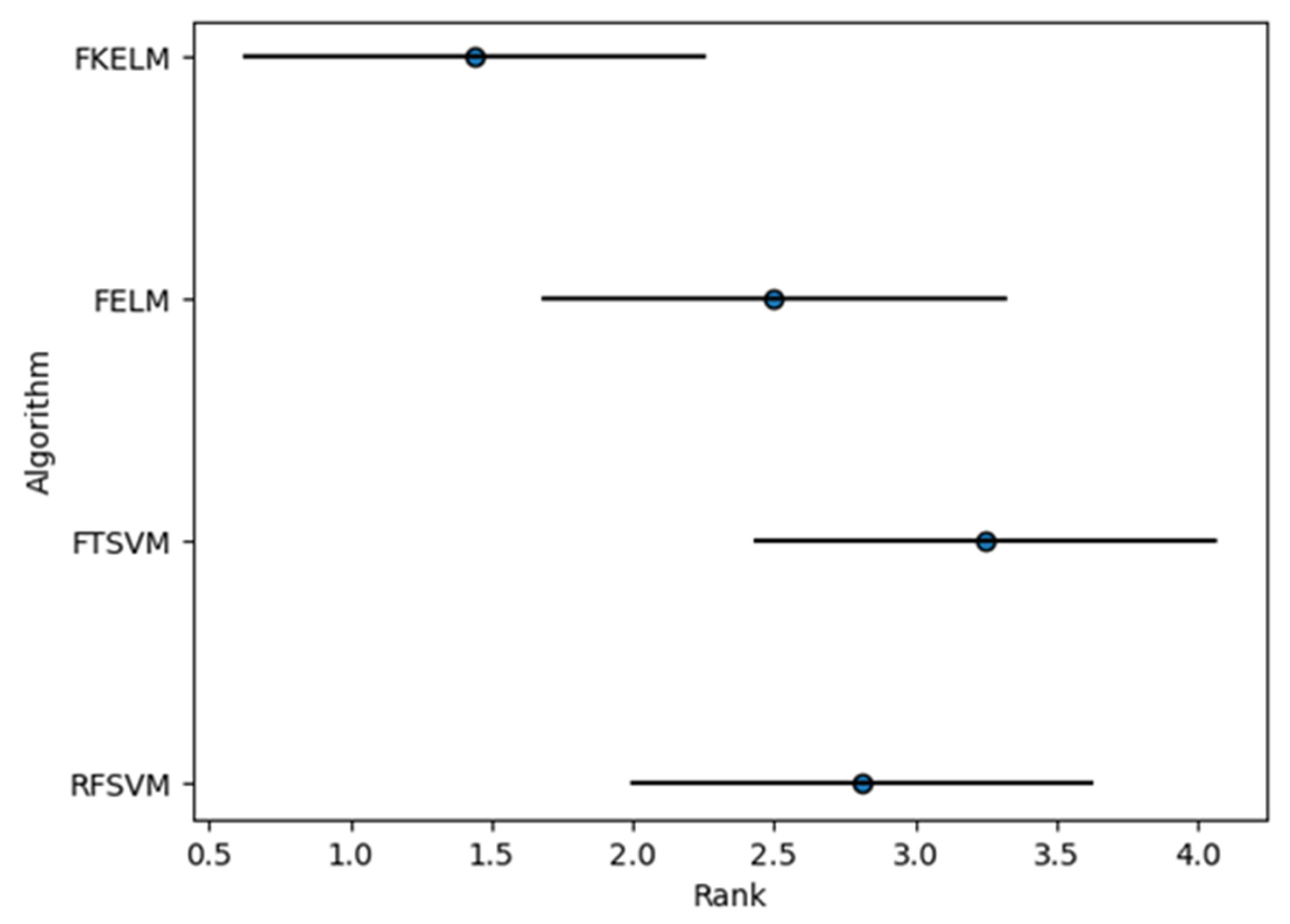
4.2. Discussion of Results

Table 5 and Table 6 and Figure 8, Figure 9, Figure 10 and Figure 11 report quantitative comparisons between all the algorithms considered, namely the RFSVM, FTSVM, FELM, and FKELM. Table 7 presents a qualitative assessment of their performance. According to the Friedman test, the FKELM is ranked first, followed by the FELM, RFSVM and FTSVM.

5. Conclusions

In general, the ELM has better generalization capacity and higher efficiency than the traditional SVM. In order to improve efficiency and classification accuracy, in this study, two new algorithms FELM and FKELM were proposed, where they used a feature ranking strategy and a memorization–generalization kernel, respectively. Both algorithms can be applied to datasets with small or medium sample sizes. The FELM and FKELM can simultaneously complete the feature selection and classification processes, improving their training efficiency.
Experiments on artificial and benchmark datasets demonstrated that the proposed approaches have higher classification accuracy and higher learning speed than the RFSVM and FTSVM. According to the Friedman statistical method and the Nemenyi classification performance test, the FKELM is ranked first, followed by the FELM, RFSVM, and FTSVM. Based on these ranks, the FKELM exhibits significantly better performance than the FTSVM, while the FELM has slightly better performance than the RFSVM and significantly better performance than the FTSVM. In most cases, the FKELM is the most accurate in the classification performance, whereas the FTSVM is the worst.
By comparing the classification accuracy on ultra-high-dimension datasets, for example, Colon and Leukaemia datasets, it was concluded that the FELM and FKELM have slightly lower performance than the RFSVM. As seen in Table 5, it can be obtained that the FELM and FKELM can complete the classification process at a significantly high learning speed. Therefore, the focuses of our future research are improving the accuracy and robustness of the proposed algorithms on such ultra-high-dimension datasets and using the feature ranking strategy on other improved ELM models. Furthermore, it should be noted that in this study, we only verified the classification accuracy. In future studies, we will also attempt to verify the regression capacity of the proposed algorithms.

Author Contributions

Conceptualization, Y.F. and Q.W.; methodology, Y.F.; software, Y.F.; validation, Y.F., Q.W., and K.L.; formal analysis, Y.F.; investigation, H.G.; resources, Y.F.; data curation, Y.F.; writing—original draft preparation, Y.F.; writing—review and editing, Y.F., Q.W., and H.G.; visualization, Y.F.; supervision, Y.F.; project administration, Q.W.; funding acquisition, Q.W. All authors have read and agreed to the published version of the manuscript.

Funding

This research was funded in part by the National Natural Science Foundation of China (grant 51875457), the Key Research Project of Shaanxi Province (2022GY-050, 2022GY-028), the Natural Science Foundation of Shaanxi Province of China (2022JQ-636, 2021JQ-701), the Shaanxi Youth Talent Lifting Plan of Shaanxi Association for Science and Technology (20220129), and the Special Scientific Research Plan Project of the Shaanxi Province Education Department (21JK0905).

Institutional Review Board Statement

Not applicable.

Informed Consent Statement

Not applicable.

Data Availability Statement

The UCI machine learning repository is available at http://archive.ics.uci.edu/ml/datasets.php (accessed on 15 October 2021). The test L Gene expression Leukaemia testing dataset was obtained from Golub. The microarray data are available at https://www.sciencedirect.com/topics/computer-science/microarray-data (accessed on 15 October 2021).

Acknowledgments

The authors thank the anonymous reviewers for their constructive comments.

Conflicts of Interest

The authors declare no conflict of interest.

References

  1. Dash, M.; Liu, H. Feature selection for classification. Intell. Data Anal. 1997, 1, 131–156. [Google Scholar] [CrossRef]
  2. Zhou, L.; Si, Y.W.; Fujita, H. Predicting the listing statuses of Chinese-listed companies using decision trees combined with an improved filter feature selection method. Knowl.-Based Syst. 2017, 128, 93–101. [Google Scholar] [CrossRef]
  3. Kang, M.; Rashedul, I.M.; Jaeyoung, K.; Kim, J.M.; Pecht, M. A Hybrid feature selection scheme for reducing diagnostic performance deterioration caused by outliers in Data-Driven diagnostics. IEEE Trans. Ind. Electron. 2016, 63, 3299–3310. [Google Scholar] [CrossRef]
  4. Zhao, J.; Chen, L.; Pedrycz, W.; Wang, W. Variational inference-based automatic relevance determination kernel for embedded feature selection of noisy industrial data. IEEE Trans. Ind. Electron. 2018, 66, 416–428. [Google Scholar] [CrossRef]
  5. Souza, R.; Macedo, C.; Coelho, L.; Pierezan, J.; Mariani, V.C. Binary coyote optimization algorithm for feature selection. Pattern Recognit. 2020, 107, 107470. [Google Scholar] [CrossRef]
  6. Sun, L.; Wang, T.X.; Ding, W.; Xu, J.; Lin, Y. Feature selection using fisher score and multilabel neighborhood rough sets for multilabel classification. Inf. Sci. 2021, 578, 887–912. [Google Scholar] [CrossRef]
  7. Binu, D.; Kariyappa, B.S. Rider Deep LSTM Network for Hybrid Distance Score-based Fault Prediction in Analog Circuits. IEEE Trans. Ind. Electron. 2020, 99, 10097–10106. [Google Scholar] [CrossRef]
  8. Jin, C.; Li, F.; Ma, S.; Wang, Y. Sampling scheme-based classification rule mining method using decision tree in big data environment. Knowl.-Based Syst. 2022, 244, 108522. [Google Scholar] [CrossRef]
  9. Rouhani, H.; Fathabadi, A.; Baartman, J. A wrapper feature selection approach for efficient modelling of gully erosion susceptibility mapping. Prog. Phys. Geogr. 2021, 45, 580–599. [Google Scholar] [CrossRef]
  10. Liu, W.; Wang, J. Recursive elimination current algorithms and a distributed computing scheme to accelerate wrapper feature selection. Inf. Sci. 2022, 589, 636–654. [Google Scholar] [CrossRef]
  11. Pintas, J.T.; Fernandes, L.; Garcia, A. Feature selection methods for text classification: A systematic literature review. Artif. Intell. Rev. 2021, 54, 6149–6200. [Google Scholar] [CrossRef]
  12. Vapnik, V.N. The Nature of Statistical Learning Theory; Springer: Berlin/Heidelberg, Germany, 1995; Volume 8, p. 1564. [Google Scholar]
  13. Jayadeva; Khemchandani, R.; Chandra, S. Twin support vector machines for pattern classification. IEEE Trans. Ind. Electron. 2007, 29, 905–910. [Google Scholar] [CrossRef] [PubMed]
  14. Huang, G.B.; Zhu, Q.Y.; Siew, C.K. Extreme learning machine: Theory and applications. Neurocomputing 2006, 70, 489–501. [Google Scholar] [CrossRef]
  15. Cui, D.; Huang, G.B.; Liu, T. ELM based Smile Detection using Distance Vector. Pattern Recognit. 2018, 78, 356–369. [Google Scholar] [CrossRef]
  16. Huang, G.B.; Zhou, H.; Ding, X.; Zhang, R. Extreme learning machine for regression and multiclass classification. IEEE Trans. Syst. Man Cybern. Part B Cybern. 2012, 42, 513–529. [Google Scholar] [CrossRef]
  17. Albashish, D.; Hammouri, A.I.; Braik, M.; Atwan, J.; Sahran, S. Binary biogeography-based optimization based SVM-RFE for feature selection. Appl. Soft Comput. 2020, 101, 107026. [Google Scholar] [CrossRef]
  18. Guyon, I.; Weston, J.; Barnhill, S. Gene selection for cancer classification using support vector machines. Mach. Learn. 2002, 46, 389–422. [Google Scholar] [CrossRef]
  19. Chang, Y.; Lin, C.; Guyon, I. Feature ranking using linear SVM. In Proceedings of the Workshop on the Causation and Prediction Challenge at WCCI 2008, Hong Kong, China, 3–4 June 2008; 2008; Volume 3, pp. 53–64. [Google Scholar]
  20. Mangasarian, O.L.; Gang, K. Feature selection for nonlinear kernel support vector machines. In Proceedings of the Seventh IEEE International Conference on Data Mining Workshops (ICDMW 2007), Omaha, NE, USA, 31 March 2008; pp. 28–31. [Google Scholar]
  21. Bai, L.; Wang, Z.; Shao, Y.H.; Deng, N.Y. A novel feature selection method for twin support vector machine. Knowl.-Based Syst. 2014, 59, 1–8. [Google Scholar] [CrossRef]
  22. Man, Z.; Huang, G.B. Special issue on extreme learning machine and deep learning networks. Neural Comput. Appl. 2020, 32, 14241–14245. [Google Scholar] [CrossRef]
  23. Adesina, A.F.; Jane, L.; Abdulazeez, A. Ensemble model of non-linear feature selection-based Extreme Learning Machine for improved natural gas reservoir characterization. J. Nat. Gas Sci. Eng. 2015, 26, 1561–1572. [Google Scholar]
  24. Vapnik, V.; Izmailov, R. Reinforced SVM method and memorization mechanisms. Pattern Recognit. 2021, 119, 108018. [Google Scholar] [CrossRef]
  25. Iosifidis, A.; Gabbouj, M. On the kernel Extreme Learning Machine classifier. Pattern Recognit. Lett. 2015, 54, 11–17. [Google Scholar] [CrossRef]
  26. UCI Machine Learning Repository. Available online: http://archive.ics.uci.edu/ml/datasets.php (accessed on 15 October 2021).
  27. Test, L. Gene Expression Leukemia Testing Data set from Golub. Available online: https://search.r-project.org/CRAN/refmans/SIS/html/leukemia.test.html (accessed on 15 October 2021).
  28. Microarray Data. Available online: https://www.sciencedirect.com/topics/computer-science/microarray-data (accessed on 15 October 2021).
  29. Hua, X.G.; Ni, Y.Q.; Ko, J.M.; Wong, K.Y. Modeling of temperature–frequency correlation using combined principal component analysis and support vector regression technique. J. Comput. Civ. Eng. 2007, 21, 122–135. [Google Scholar] [CrossRef]
  30. Demšar, J. Statistical comparisons of classifiers over multiple data sets. J. Mach. Learn. Res. 2006, 7, 1–30. [Google Scholar]
  31. Iman, L.; Davenport, J.M. Approximations of the critical region of the Friedman statistic. Commun. Stat. A 1998, A9, 571–595. [Google Scholar]
  32. Zheng, F.; Webb, G.I.; Suraweera, P.; Zhu, L. Subsumption resolution: An efficient and effective technique for semi–naive Bayesian learning. Mach. Learn. 2012, 87, 93–125. [Google Scholar] [CrossRef]
Figure 1. The flow chart of feature selection.
Axioms 11 00444 g001
Figure 2. The basic structure of an ELM.
Axioms 11 00444 g002
Figure 3. Comparison among three kernels: (a) generalization RBF kernel; (b) memorization RBF kernel; (c) memorization-generalization kernel.
Axioms 11 00444 g003
Figure 4. Relationship between the number of hidden layer nodes and the classification accuracy of FELM.
Axioms 11 00444 g004
Figure 5. Relationship between the number of hidden layer nodes and the classification accuracy of FKELM.
Axioms 11 00444 g005
Figure 6. Classification results obtained with the two-moon dataset using: (a) RFSVM; (b) FTSVM; (c) FELM; (d) FKELM.
Axioms 11 00444 g006
Figure 7. Classification results obtained with the self-defining function dataset using: (a) RFSVM; (b) FTSVM; (c) FELM; (d) FKELM.
Axioms 11 00444 g007aAxioms 11 00444 g007b
Figure 8. Comparison of the accuracy of different algorithms when classifying the training datasets.
Axioms 11 00444 g008
Figure 9. Comparison of the accuracy of different algorithms when classifying the test datasets.
Axioms 11 00444 g009
Figure 10. Comparison of the computational cost of different algorithms on all the datasets.
Axioms 11 00444 g010
Figure 11. Friedman test chart.
Axioms 11 00444 g011
Table 1. Functions used for generating the dataset.
DatasetFunction Definition
Self-defining function covariance   1                   0               0 1
mean value (0,0) and (0.8,0.8)
Two-moon r U r w 2 , r + w 2
θ 1 U ( 0 , π ) θ 2 U ( π , 0 )
Table 2. Details of the artificial dataset.
DatasetNumber of
Test Samples
Number of
Training Samples
Range of
Independent Variables
Self-defining function50350 x 0 , 2
Two-moon100501 x 0 , 4.5
Table 3. Experimental results from the artificial dataset.
DatasetAlgorithmTraining
Accuracy
Test
Accuracy
Time (s)Parameters
( C , C 1 , C 2 , ψ , σ , τ )
Two-moonRFSVM0.99480.96000.86322–8, –, –, 22, 2–3, –
FTSVM1.00000.98190.6929–, 2–3, 22, 21, 2–3, –
FELM1.00001.00000.32082–6, –, –, 22, 2–1, –
FKELM1.00001.00000.35242–6, –, –, 22, 2–1, 0.3
Self-defining functionRFSVM0.89770.90120.50072–7, –, –, 20, 2–3, –
FTSVM0.92930.91100.2410–, 20, 23, 21, 2–4, –
FELM0.99220.98790.13752–5, –, –, 22, 2–2, –
FKELM0.99720.99130.13982–5, –, –, 22, 2–2, 0.4
Table 4. Details of the benchmark datasets analysed.
DatasetNumber of
Test Samples
Number of
Training Samples
Number of Features
Australian20748314
Heart8118913
Ionosphere10524633
WDBC17139830
WPBC5913934
Sonar6214660
Colon18442000
Leukaemia21517129
Table 5. Experimental results on the benchmark datasets.
DatasetAlgorithmTraining
accuracy
Test
accuracy
Time (s)Parameter
(C,C1,C2,Ψ,σ,τ)
AustralianRFSVM0.86170.83103.409224, –, –, 22, 2–7, –
FTSVM0.86380.85732.2620–, 23, 25, 22, 2–8, –
FELM0.87320.86620.56122–5, –, –, 21, 2–1, –
FKELM0.87070.85950.64252–5, –, –, 21, 2–1, 0.6
HeartRFSVM0.84960.84853.865921, –, –, 21, 2–7, –
FTSVM0.83700.83212.2051–, 22, 22, 21, 2–9, –
FELM0.87590.86790.15282–2, –, –, 20, 2–2, –
FKELM0.87960.87850.16072–2, –, –, 20, 2–2, 0.4
IonosphereRFSVM0.89570.89125.90612–1, –, –, 20, 2–3, –
FTSVM0.90070.89764.5770–, 20, 23, 22, 2–2, –
FELM0.87290.87280.60122–5, –, –, 22, 2–2, –
FKELM0.91570.90720.63142–5, –, –, 22, 2–2, 0.4
WDBCRFSVM0.95970.95370.33722–2, –, –, 21, 2–3, –
FTSVM0.95730.95860.1798–, 20, 20, 21, 2–4, –
FELM0.95920.95180.014623, –, –, 20, 2–5, –
FKELM0.98230.97620.017725, –, –, 20, 2–5, 0.5
WPBCRFSVM0.79920.80342.500727, –, –, 21, 2–5, –
FTSVM0.81410.82021.5451–, 25, 26, 21, 2–5, –
FELM0.84220.83970.127923, –, –, 21, 2–8, –
FKELM0.84090.85130.139823, –, –, 21, 2–8, 0.3
SonarRFSVM0.79720.79112.983222, –, –, 20, 2–3, –
FTSVM0.89330.88491.7132–, 21, 25, 21, 2–2, –
FELM0.89950.88790.137523, –, –, 22, 2–4, –
FKELM0.91720.90130.145224, –, –, 22, 2–4, 0.5
ColonRFSVM0.85830.85120.516022, –, –, 20, 21, –
FTSVM0.72080.70100.3197–, 20, 23, 21, 20, –
FELM0.78820.78710.01332–1, –, –, 22, 22, –
FKELM0.79710.79220.01392–1, –, –, 22, 20, 0.6
LeukaemiaRFSVM0.82350.80170.920927, –, –, 23, 2–5, –
FTSVM0.62930.61100.5244–, 25, 26, 23, 2–5, –
FELM0.64710.65720.039924, –, –, 24, 2–6, –
FKELM0.68820.69380.045124, –, –, 24, 2–5, 0.6
Table 6. Average accuracy ranks.
DatasetRFSVMFTSVMFELMFKELM
AustralianTraining4312
Test4312
HeartTraining3421
Test3421
IonosphereTraining3241
Test3241
WDBCTraining2431
Test3241
WPBCTraining
Test
4
4
3
3
1
1
2
2
SonarTraining4321
Test4321
ColonTraining1432
Test1432
LeukaemiaTraining1432
Test1432
Average rank 2.81253.252.51.4375
Table 7. Qualitative assessment of the different algorithms.
AlgorithmSize of DatasetTimeClassification Performance
RFSVMSmall and medium samplesMuchPoor
Large samplesMuchSightly good
FTSVMSmall and medium samplesMediumPoor
Large samplesMediumPoor
FELMSmall and medium samplesLittleSignificantly good
Large samplesLittleGood
FKELMSmall and medium samplesLittleSignificantly good
Large samplesLittleGood
Publisher’s Note: MDPI stays neutral with regard to jurisdictional claims in published maps and institutional affiliations.

