1. Introduction
Waves on the surface of rivers, seas and oceans became one of the main objects of theoretical research as the first fundamental equations of continuum mechanics and closed systems of equations were formulated [
1,
2,
3]. Due to a large difference in the physical properties of the atmosphere and water [
4], the theory of waves evolved with the approximation of the homogeneity and immutability of the density of the contacting media. B. Franklin in the 18th century observed the water–olive oil interface motion in a ship’s lighting lamp and pointed out that the variability of density with depth should be taken into account when analyzing the wave phenomena in a liquid [
5].
The results of the analysis of the first papers, which considered the variability of the density of the liquid in depth, were presented [
6], but for some unknown reason, mathematicians and mechanics did not pay attention to these topics. For example, such a fundamental characteristic as the buoyancy frequency calculated in [
7], which is the limiting frequency for propagating internal waves in a continuously stratified fluid, escaped from attention. Independently the buoyancy frequency was re-discovered as the natural oscillation frequency of probe balls drifting in a stratified atmosphere [
8] and later it was associated with the local extreme in the spectrum of high-frequency pressure oscillations recorded by a microbarograph [
9].
Due to the practical importance of the issue, for a long time, researchers have been concentrating their efforts on studying periodic phenomena in a liquid in the context of the force action of waves on obstacles and the wave resistance of bodies moving in a liquid. The scientists assumed the constancy of density and incompressibility of the liquid [
10] to be the most important qualities. Nowadays the constant density approximation is still considered high priority in the description of wave processes [
11].
In theoretical works much attention is paid to the study of nonlinear properties of waves. The first heuristic discovery—the theory of periodic nonlinear vortex waves [
12]—is significant in wave theory development. The approach was extended in [
13,
14], then analyzed in [
15] and it has recently been supplemented with new results [
16,
17]. Another large cycle of studies of nonlinear waves, initiated by observations of a solitary wave in a shipping channel [
18], is successfully proceeding at the present time. The number of various model equations [
19,
20] for the description of nonlinear wave properties is continuously increasing [
21].
Seminal works [
22,
23] occupied a special place among the first publications. In these studies, the parameters of infinitesimal waves were determined, the waves of finite amplitude were calculated and showed the existence of the wave transfer of matter (Stokes drift) using the methods of the regular perturbations theory. The mass transfer is caused by nonlinear effects, which are distinctly revealed in the deviation of the waveform from the ideal one, i.e., in a nonlinear wave, the crests become sharper, and the troughs become flatter. The limiting angle between the tangents to the right and left sides of the crest is calculated as
in [
23], and as
in [
13]. It depends on the nonlinearity parameter
[
24] when describing the propagating potential waves of finite amplitude by means of Lambert’s complex functions (
and
are the amplitude and frequency of the wave,
is the gravity acceleration).
Calculations of the viscous attenuation of waves in a deep liquid and a channel of finite depth were carried out by asymptotic methods in a linear and nonlinear formulation [
6,
25,
26]. Such calculations continue to be conducted at the present time using various approximations [
27,
28,
29,
30].
The “boundary layer” ideas (i.e., a mathematical model of the flow adjacent to the surface of the liquid, in which the influence of viscosity is considerably revealed), which were formulated at the beginning of the 20th century, had a significant impact on the development of the theory of waves in a liquid. The approximation of the boundary layer, accompanied by the reformulation of the defining equations [
31], stimulated the development of the search for new analytical methods of finding their solutions [
32]. The analysis of the wave equations by the theory of regular perturbations methods showed that in a homogeneous liquid with kinematic viscosity
, a surface gravitational wave with a frequency
is accompanied by a boundary layer with a specific thickness
. Separate boundary layers are formed on the free surface and on the solid bottom of the channel through which the waves propagate [
33].
The boundary layer greatly influences all the parameters of fluid flows, namely pressure distribution, velocity and substance transfer characteristics [
34]. Corrections of the theory formulas [
33] due to the viscous attenuation of waves were later calculated in the second order of the perturbation theory [
35]. The analysis of the dispersion relation for surface gravitational waves and accompanying boundary layers in a viscous liquid, supplemented by calculations of the attenuation coefficient and the scale of spatial attenuation of the wave was carried out in [
36].
A more complex model of a “double boundary layer”, inside which there is a periodic boundary layer with a length scale
, was proposed to describe standing waves [
37].
With the frequency increasing, the surface tension influences more the pattern of waves on the surface of the liquid. The surface tension coefficient
is a parameter that determines the type of dispersion relation for short waves [
38] and accompanying fine constituents [
39]. The surface tension changes the dependences of the group and phase velocity, the attenuation coefficient and the velocity of matter transfer
on frequency
, wave vector
or wavelength
. The pattern of waves generated by a short-range localized source in a viscous liquid, taking into account the effects of surface tension, was calculated in [
40].
The data of the first systematic experimental studies of surface waves, which were conducted in laboratory basins at the end of the 19th century [
41], generally showed satisfactory agreement with the calculations of velocity in the liquid thickness [
23]. The visualization of the velocity profile using a “marker” (i.e., a colored wake of a submerging particle) showed the existence of a drift in the near-surface and bottom layers in the direction of wave propagation and slow counterflow in the middle of the liquid layer [
42]. Additional cleaning from dust and film of the target liquid surface and consideration of viscous attenuation in the calculations of the near-surface boundary layer significantly reduced the difference between the data of calculations and experiments in a laboratory channel [
43]. The observations of rearrangement of the distribution pattern of initially homogeneous suspension in the field of standing gravity waves in a vertically oscillating basin are given in [
44].
In the field of propagating gravitational-capillary waves (
), the substance of the colored drop is distributed unevenly over the surface of the primary cavity [
45], the same as in the case of a drop merging with a target liquid at rest [
46]. In the evolutionary process a slowly drifting colored primary contact area, a near-surface jet with a vortex head and a sinking ring vortex remain in the distribution pattern of the substance. There is a pronounced fibrous structure in the distribution of the drop substance in the target fluid [
45].
Widespread capillary waves, which are observed in various rivers, seas and oceans, are caused by weak wind gusts in calm [
47] and are certainly present on the slopes of large gravitational waves [
48] in the stormy open ocean [
49] and coastal regions [
50]. Capillary waves contribute to the formation of bubbles, drops and foam [
51] and participate in the processes of generating sound packets when drops fall [
52]. Drop impact sounds form rain noise [
53], which is one of the main sources determining the acoustic background of the ocean [
54].
The capillary ripples determine the roughness and the real area of the contact surface. The estimation of their influence on the transfer of momentum, energy and matter between the atmosphere and the hydrosphere is of scientific and practical interest. A continuously expanding list of scientific tasks supports the interest in studying the dynamics of capillary waves in a wide range of conditions.
The analysis of the additional dissipation of short gravitational and gravitational-capillary waves caused by “parasitic” capillary waves on the slopes of longer waves in a laboratory pool are given in [
55]. The presence of a surfactant film dampens short capillary waves, which in turn amplifies decimeter waves [
56]. The discussion of modern optical methods for studying capillary waves and the data of detailed experiments is carried out in [
57]. A review of papers on the nonlinear interaction of coexisting waves of different frequencies within the framework of the theory of “wave turbulence” is presented in [
58]. The basic mechanism of energy transfer in weak turbulence theory is validated experimentally in the gravity (four-wave interactions) and capillary (three-wave interactions) regimes. Advanced experiments enable the achievement of full spatiotemporal reconstruction of the wave field in a weakly or strong nonlinear regime, to infer wave statistics as well as waves’ nonlinear dispersion relationship, to compare with theory [
58]. The study in [
59] discusses the influence of attenuation on nonlinear interactions of short waves and surface waves and the properties of “wave turbulence”. In all cases, the density of the liquid is assumed to be homogeneous.
However, in real conditions, the influence of differences in atmospheric and hydrosphere temperatures, insolation, radiative heat transfer, variability in the concentration of dissolved and suspended particles and flows ensure the heterogeneity of the density profile throughout the depth of the liquid [
60]. The same happens in a thin near-surface layer, where temperature changes rapidly with depth and forms a “cold” or “warm” film [
61].
The given study of the properties of surface waves and accompanying fine components in a viscous stably stratified liquid is based on a complete system of fundamental equations, which was firstly collected in [
62] and later was considered in [
63,
64]. In this paper, a reduced system of the fundamental equations in which the density variability is preserved without considering variations in temperature, salinity or pressure that cause it to change is used. This system of equations is analyzed by methods of the singular perturbations theory [
65] taking into account the compatibility condition [
66], enabling calculation of both the waves themselves and the family of accompanying fine constituents (i.e., ligaments).
Analysis of the solutions of the fundamental equations system in a continuously stratified fluid has shown that for periodic flows (with a frequency less than the buoyancy frequency), regular solutions describe waves. The wave frequency
is related to the wave number
by an algebraic dispersion relation
, which may include the amplitude
[
66,
67].
Singular solutions describe ligaments perturbations—extended in some direction and fine in others—outlining wave beams. The transverse scale of the ligaments
is determined by the kinematic viscosity of the liquid
and the wave frequency
:
(Stokes scale) or equivalent parameter with the buoyancy frequency
:
. The number and positions of the ligaments in space are determined by the geometry of the source, the amplitude and frequency of its oscillations. Calculations of internal wave beams and accompanying ligaments in stratified liquids and gases are given in [
68,
69].
In this paper, a dispersion equation in a linear approximation for two-dimensional periodic perturbations on the surface of a viscous exponentially stratified liquid is constructed for the first time. The properties of its complete solutions are analyzed. Approximate solutions are obtained by perturbation theory. Regular solutions describe waves in the range from infra-low frequency to gravitational-capillary and capillary waves. The dispersion relations continuously transform into the well-known formulas of the theory of waves in a homogeneous viscous or ideal liquid. Singular solutions characterize ligaments—fine constituents that complement waves. Graphs of the dependence of the wavelengths and ligaments on the frequency, phase and group velocity of the constituents on the wavelength are given. The results can be used to solve problems of generation and propagation of surface waves with physically justified initial and boundary conditions and comparison with a high-resolution experiment.
2. Periodic Flows in a Viscous Exponentially Stratified Fluid
We consider the propagation of periodic perturbations over the surface of a viscous exponentially stratified fluid in a uniform gravity field. The undisturbed liquid filling the lower half-space is regarded to be incompressible; meanwhile the effects of thermal conductivity and diffusion are neglected.
We perform the study in a Cartesian coordinate system in which the plane coincides with the equilibrium position of a free surface of the liquid, and the axis is directed vertically upwards against the direction of the gravity acceleration The undisturbed density distribution over depth is exponential . It is characterized by reference density (i.e., the density value at the equilibrium level ), as well as the scale frequency and buoyancy period .
Mostly, changes of real fluids density are usually small and produce a small impact on the inertial properties of the flows. Nevertheless, the conservation of terms describing the stratification effects in the governing equations set is important since gravity acceleration is large. In this regard, it is useful to consider three types of medium: stratified fluids when buoyancy scale
, frequency
and period
which are included in the list of main parameters; then very weakly stratified fluids, when the scale of buoyancy substantially exceeds the values of other length scales of the problem (so called potentially homogeneous fluid) and actually homogeneous liquid whose density is assumed to be constant in the entire space [
70]. Using a weak but variable density helps to save the rank of complete non-linear set and order of the linearized set of governing equations [
66,
71] and analyzes additional solutions which are lost in approximation of homogeneous fluid.
Depending on the magnitude of the density gradient created by the corresponding temperature or salinity distributions, it is customary to distinguish strongly and weakly stratified fluids, as well as potentially and actually homogeneous fluids. The values of the characteristic physical quantities are given in
Table 1 [
70].
Strong stratification (
) is created in laboratory installations. Relatively weak stratification (
) is observed in natural conditions.
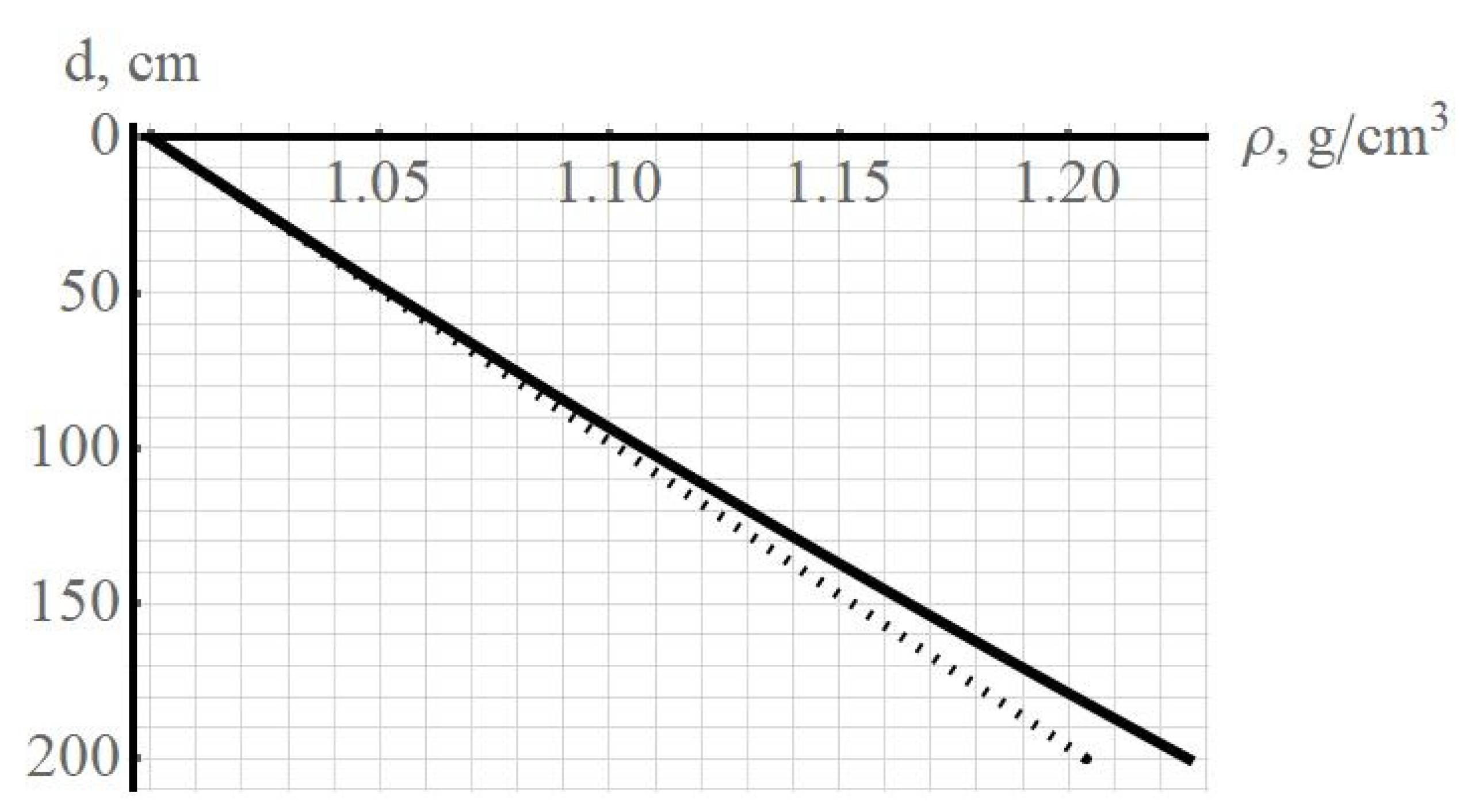
Figure 1 shows the density–depth dependencies for exponential stratification (solid line) and for linear stratification (dotted line) for a strongly stratified fluid
.
To compare the properties of exponentially and linearly stratified media, we analyze the changes in the density gradient with depth. For exponential stratification, the magnitude of the density gradient depends on the vertical coordinate
.
For linear stratification, the density gradient does not depend on the depth:
For small variations
the dependencies of the density gradient are not distinguishable for exponential and linear stratification. The exponent can be represented as a Taylor series expansion over a small parameter
and expression (1) will be written as follows:
The numerical values for the stratification scale for a strongly stratified fluid are , and for a weakly stratified fluid . At depths of less than 10% of the stratification scale, it can be argued with a high degree of accuracy that the calculations in the model of a linearly stratified fluid and exponentially stratified fluid coincide.
We study below two-dimensional periodic flows of the form
with a positive definite frequency
and a complex wave number
, the imaginary part of which characterizes the spatial attenuation of the flow. The disturbances which are homogeneous in the direction of the transverse horizontal coordinate
are selected. They include the displacement of the free surface position
. The velocity
with horizontal and vertical velocity components
in an incompressible fluid (
) is represented by derivatives of the stream function
:
The expression for the density of the liquid
replacing the equation of state in [
66] includes the initial distribution
and the perturbation caused by the examined periodic flow
.
Taking into account these assumptions, the system of continuity and Navier–Stokes equations is extremely simplified and takes the traditional form [
62,
63,
69]:
Kinematic and dynamic boundary conditions on a perturbed surface are traditional [
62]:
where
is the hydrodynamic pressure,
is the total coefficient of the surface tension of the liquid,
and
are the vectors of the external normal and tangent to the free surface of the liquid, respectively.
The studied problem includes the following dimensional parameters: density and its gradient , dynamic and density-normalized kinematic viscosity , gravity acceleration , surface tension coefficient and density-normalized surface tension coefficient , amplitude , frequency period and wavelength . The wave is also characterized by a wave vector , the modulus of which is related to the wavelength .
In the transition to a mathematical description, physical quantities serve as the basis for the introduction of characteristic scales of length, time and speed. These scales are used in the physical interpretation of the results obtained, assessing the degree of influence of various physical factors.
The degree of relative influence of viscosity and gravity on fluid flows is characterized by the scale
that appears in [
71].
Traditionally, stratification is characterized by its own length scale which takes into account or neglect the effects of compressibility, the frequency
, period
and the inverse value of the buoyancy frequency
. The stratification itself is characterized by a combinational viscous wave scale
[
72,
73], as well as a length scale
– a functional analogue of the dissipative Stokes microscale
.
The dualism of the nature of surface waves, whose properties depend on the gravity acceleration , normalized coefficients of surface tension and kinematic viscosity results in the introduction of several scales, including the capillary length . The inequality indicates the severity of surface force effects, and —indicates the severity of gravitational effects.
The structure of near-surface flows is also characterized by a known proper velocity scale and an additional time scale of kinematic nature .
Wave propagation is characterized by group and phase velocity .
Ratios of uniform scales form a set of dimensionless parameters, parts of which are used in further calculations.
2.1. Equations of Periodic Flows and Dispersion Relations for Plane Infinitesimal Waves
To simplify expressions, we accept the initial density distribution to be exponential, as it is customary in most models:
The change of variables proposed in [
74] allows the transformation of the equations of motion for an arbitrary smooth density profile into equations with constant coefficients that determine the preferential choice of the exponential density profile.
Further calculations are carried out in the Boussinesq approximation, considering the smallness of absolute density variations in stratified media (in particular, a small value of the wavelength and buoyancy scale ratio
). The density variations are neglected everywhere, except for the term with a large coefficient (i.e., the gravity acceleration
). In this approximation, the system (5) takes the form:
In a linear approximation the system (8) reduces to:
Cross-differentiation of spatial coordinates of the upper and middle equations of the system (9) allows getting rid of pressure:
Subtraction of the second equation, differentiated by coordinate and multiplied by a coefficient
from the first equation of the system (10), differentiated by time, allows getting rid of the function
:
Equation (11) takes the next form for an exponentially stratified fluid (7):
The boundary conditions (6) for all variables of the infinitesimal waves
are traditionally carried away from the wave surface
to the unperturbed level
and take the form
The small coefficient (kinematic viscosity
), which ensures slow attenuation of the wave as it propagates in the liquid, allows the classification of the system (12) as a system of singularly perturbed equations and the application of the theory of singular perturbations [
65] for its analysis. The compatibility condition, which requires the analysis of all the roots of the dispersion equation and the system (12) solutions, should be taken into account [
66].
For surface waves with
, the solution of Equation (12) is sought in the form of plane waves:
Here corresponds to the regular solution of the dispersion equation, and corresponds to the singular solution of the dispersion equation.
We obtain the shape of the deviation of the free surface of the liquid, the condition of the relationship between the amplitudes of the regular and singular component by substituting (14) into Equation (12) and boundary conditions (13):
as well as the dispersion relations:
Calculated for the first time the expressions (16) are transformed into the relations for a viscous homogeneous fluid and for an ideal exponentially stratified fluid in limiting transitions
and
respectively. Similar dispersion relations for internal waves and ligaments in the thickness of a stratified fluid were presented in [
75].
2.2. Solution of the Dispersion Equation
It is convenient to analyze the dispersion relations (13) in a dimensionless form. The time scale will be the parameter, which is inverse to the buoyancy frequency
, and the viscous wave scale
is chosen as the length scale. The ratios of the eigenscales of the problem
and
are used to construct new dimensionless parameters
involved in further calculations. Then, expressions (16) could be rewritten in a dimensionless form:
The upper dispersion relation in (17) has regular solutions, which we have denoted
, and singular solutions, which are denoted
. For a large number of real liquids, the parameter
and regular solutions are found by direct decomposition over a small parameter
:
Substituting (18) into the upper expression in (17) we obtain up to the terms of the order
:
Since the equations in the system (17) have the fourth degree, it is necessary to find two more solutions, which are singular perturbed ones in the form of decomposition [
65]:
The parameter
in (20) is chosen in such a way that at the highest degree the main term of the decomposition persists. Substituting instead of
in the upper expression in (17)
and equating the exponents
in different terms we get:
At the highest degree, the main term of the decomposition remains only at
. Substituting the value
in (20) and then in (17) up to the terms of the order
we get:
Leaving only the main terms of
in the lower dispersion relation (17), we obtain the dispersion equation for the regular part of the solution:
For the singular part of the solution, leaving only the main terms of the expansion of
, we obtain:
The solution of the dispersion Equation (23) for the regular wave part is:
From the condition of the physical realization of the solution (i.e., the damping of the flow with depth) it follows that only roots with
possess a physical meaning. Decomposing the solution (25) for the regular wave part into a Taylor series, we obtain:
With consideration of (19) and the condition
, it can be seen that we implement only one root of (26) and finally for the regular wave solution we get:
We perform similar transformations for singular ligament-solution. The solutions (24), which are found taking into account (22) and the conditions of the physical implementation of the roots
of the singular ligament, take the form:
Expressions (27), (28) describe new dispersion relations for surface waves (27) and associated ligaments (28) in a viscous exponentially stratified fluid.
2.3. Low Frequency Waves
The solution for low frequency waves (
) is sought as the sum of the propagation of gravitational waves (waves with wave number components
) and fine perturbation (with wave number component
) as well:
Substituting (26) into (9) leads to dispersion relations:
Substituting solution (29) into the boundary conditions (13), we obtain an expression for the shape of the free surface and additional relations. These additional relations determine the relationship between the amplitudes of the various components of periodic motion:
In a dimensionless form, the dispersion relations (30) take the form:
The expressions for the surface component of periodic motion, up to the notation, coincide with the dispersion equations of surface waves discussed above. For low frequency waves, we will look for regular wave solutions in the form of expansion (18) and up to the terms of the order
:
Similarly to surface waves case, we find singular solutions of the dispersion equation for low frequency waves using decomposition (20). Just as in the case of high frequency surface waves
, the exponent of the degree
is the only one that satisfies the condition of the main term of the decomposition at the highest degree
. Making a substitution up to the terms of the order
we get:
From the relation (32) we obtain that
From the ratio (33) follows:
In the low viscosity approximation, we obtain that
The relations (40) correspond to the situation when all the energy is concentrated in gravitational waves.
2.4. Periodic Flows on the Surface of a Viscous Exponentially Stratified Liquid
First of all, let us consider the dependence of the wavelength
on the frequency of the wave motion
. We define the wavelength as follows:
This method of determination of the wavelength is due to the fact that the imaginary part of the wave number
component and the real part of the wave number
component are responsible for the spatial attenuation of motion and are not impactful to wave propagation. Substituting the dispersion relations (27) in (32), we can construct the desired dependencies.
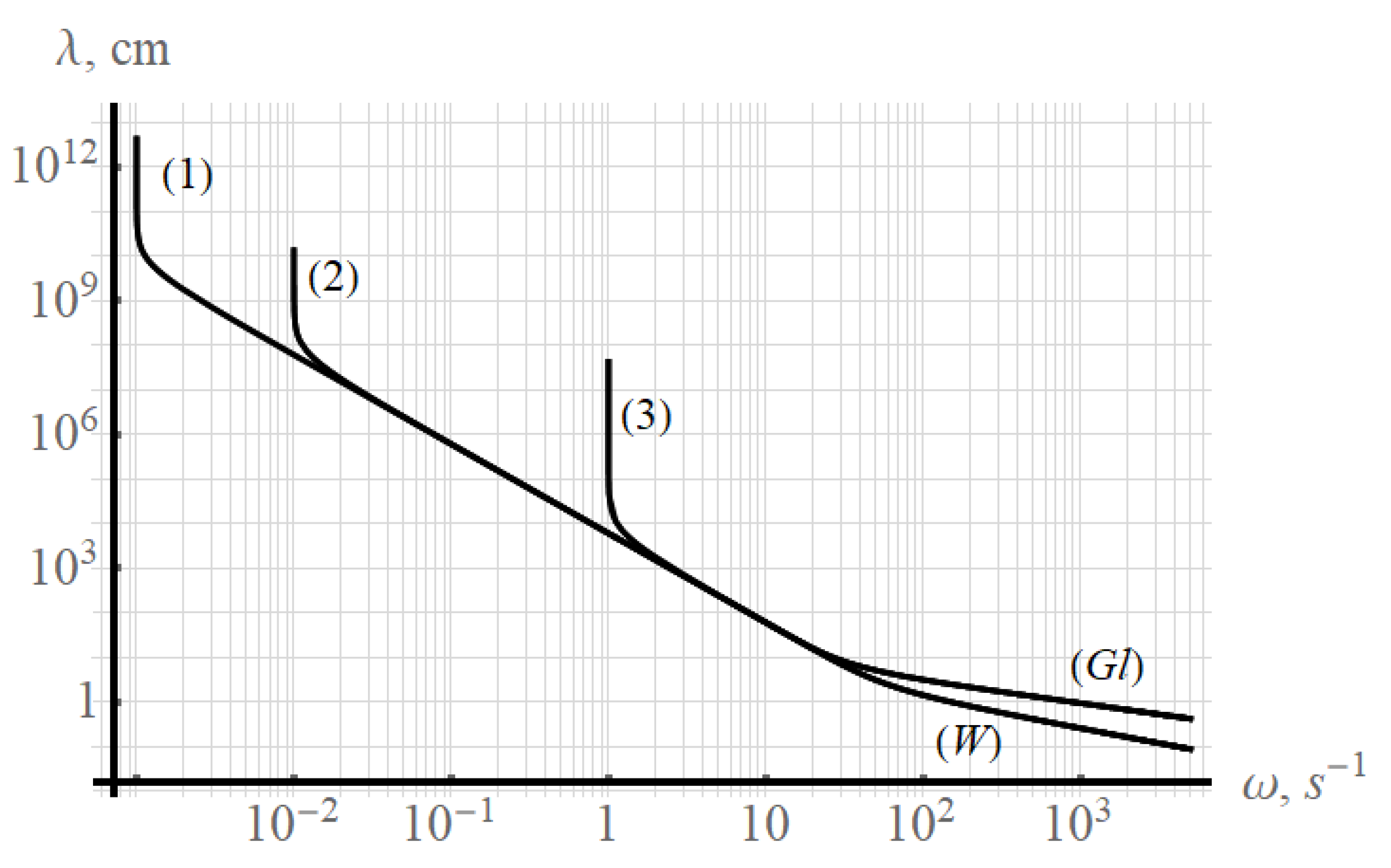
Figure 2 shows the dependence of the wavelength on the frequency of wave motion
.
The velocity of movement of the phase front of structures (wave and ligament) and the rate of energy transfer are of particular interest. The phase front moves with the phase velocity of the wave (and its analogue for the singular solution):
The energy is transferred with a group velocity
, which is defined as follows:
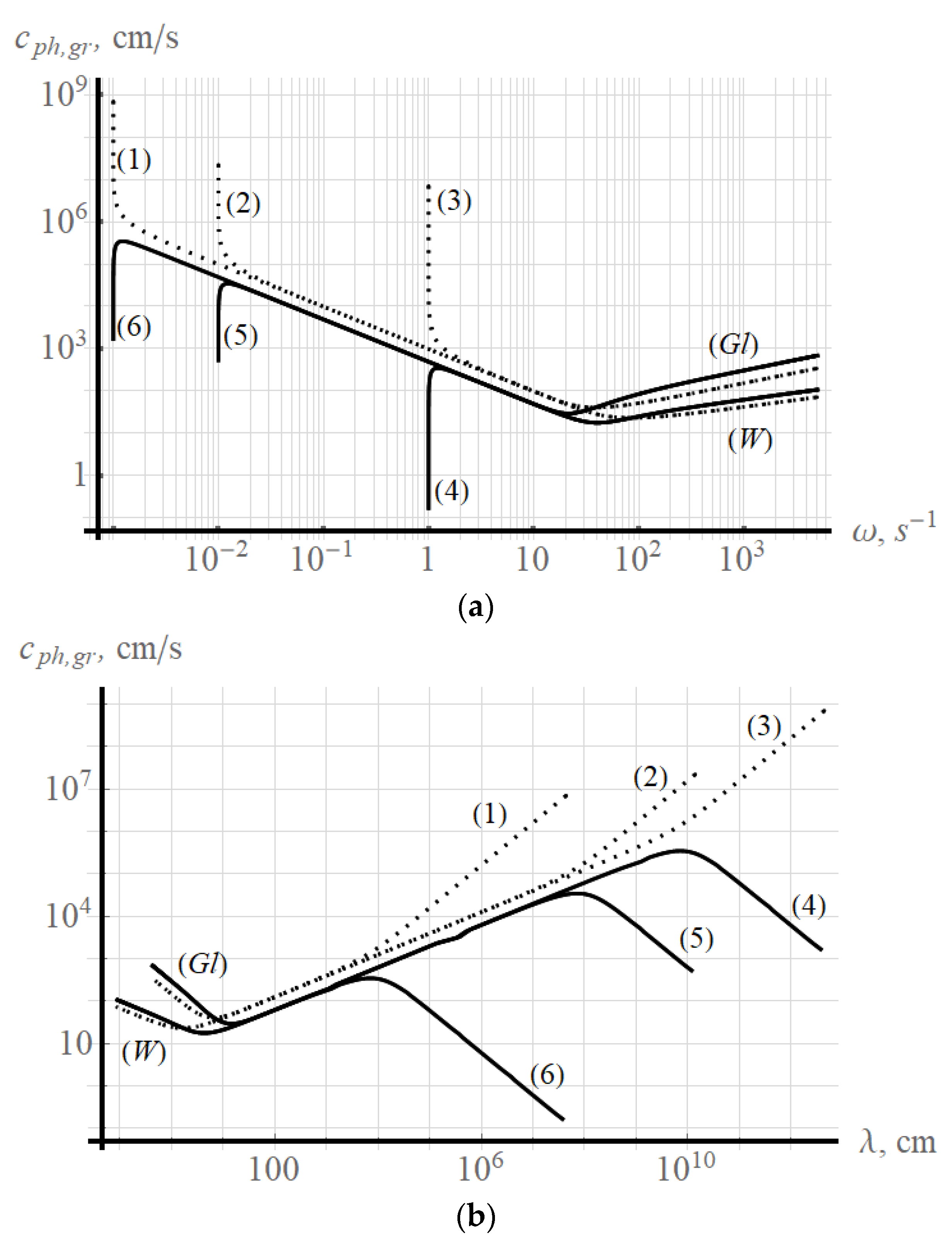
Figure 3 shows the dependencies for the phase (dashed line) and group (solid line) velocities.
Figure 2 and
Figure 3 show that viscosity has a noticeable effect on capillary waves with a wavelength
, and the stratification influences the waves with frequencies close to the buoyancy frequency
. With the advent of stratification, a forbidden part of the spectrum appears for surface waves (with frequencies lower than the buoyancy frequency). With the tending to the stratification frequency, the group velocity goes to zero, and the phase velocity tends to infinity. A similar pattern is observed when electromagnetic waves propagate in waveguides. The size of the waveguide sets a certain critical size, beyond which the electromagnetic wave does not propagate in the waveguide channel. In stratified fluids, this mechanism is not due to external geometric constraints, but is determined by the characteristics of the medium (stratification).
3. Reduction to Approximation of Actually Homogeneous Fluid
The fine constituents of periodic flows—ligaments—are a consequence of the dissipative properties of the medium, which exist not only in stratified, but also in homogeneous liquids. They are described by singular solutions of dispersion equations, the appearance of which can be observed experimentally in the structure of flows in an inhomogeneous medium. If the effects associated with buoyancy are neglected, then the density of the liquid can be considered as actually homogeneous:
and the basic equations of motion are simplified. For a viscous homogeneous liquid in a 2D formulation in a linear approximation equations for the stream function are shortened to:
Equation (45) can also be obtained by performing a limiting transition
in (12). The boundary conditions that are removed to the equilibrium surface in the case of a homogeneous liquid are as follows:
Similarly to the basic equations of motion, the boundary conditions (46) can also be obtained from the boundary conditions (13) using a limit transition
. Substitution of the solution in the form of a propagating wave
in (45) leads to dispersion relations between the components of the wave number:
The relation (48) naturally decomposes into two solutions:
Here, the reassignment of one solution
into
is introduced. The component
corresponds to the wave solution, and the component
corresponds to the ligament solution. Taking into account (49), the solution of the problem in the form of a propagating wave is transformed into:
Substituting (50) into the kinematic boundary condition, we obtain the relationship between the amplitudes of the velocity field and the deviation of the free surface from the equilibrium value:
and substitution of (50) into the dynamic condition for tangential tensions leads to the expression for the amplitude of the ligament component:
Getting rid of the pressure in the dynamic boundary condition and taking normal components, we rewrite it as:
Substituting the solution (50) into the boundary conditions (53) taking into account (49) leads to the dispersion relation for the wave constituent:
and ligament constituent:
It can be noticed that Equations (54) and (55) are also obtained from (16) with a limit transition . Further we will transfer the dispersion relations (54) and (55) to dimensionless forms in the same way as it has been done in the previous paragraph. We will choose our own viscous scale as the length scale, and the ratio as the time scale will be and the decomposition parameter .
In a dimensionless form, the conventional dispersion Equation [
15] for the wave component of the solution will be rewritten taking into account (54):
The solution of Equation (56) is obtained by the standard method and takes the form:
Decomposition (57) into a Taylor series by a small parameter
at least up to the summands
gives the expression:
Decomposition of the roots (58) into a Taylor series by a small parameter
at least up to the summands
gives the expression:
As it follows from the condition of the physical realization of the roots , considering the positive definite frequency of the wave motion, only one root, which is given by the expression (57), can be physically realized This solution describes the wave part of a periodic motion in a liquid.
To analyze the dispersion equation for a ligament solution (55) and carry out the nondimensionalization procedure, the characteristic scales can be selected the same as in the wave solution. Then in a dimensionless form, the dispersion equation (55) is written as:
Equation (61) has four roots. The analysis shows that the spatial attenuation condition is satisfied for one root only. Due to the cumbersomeness of the expression, the calculated solution is not given here.
Let us construct the dispersion dependences of the components of periodic motion in log–log scales in dimensional variables for liquids with glycerin and water parameters.
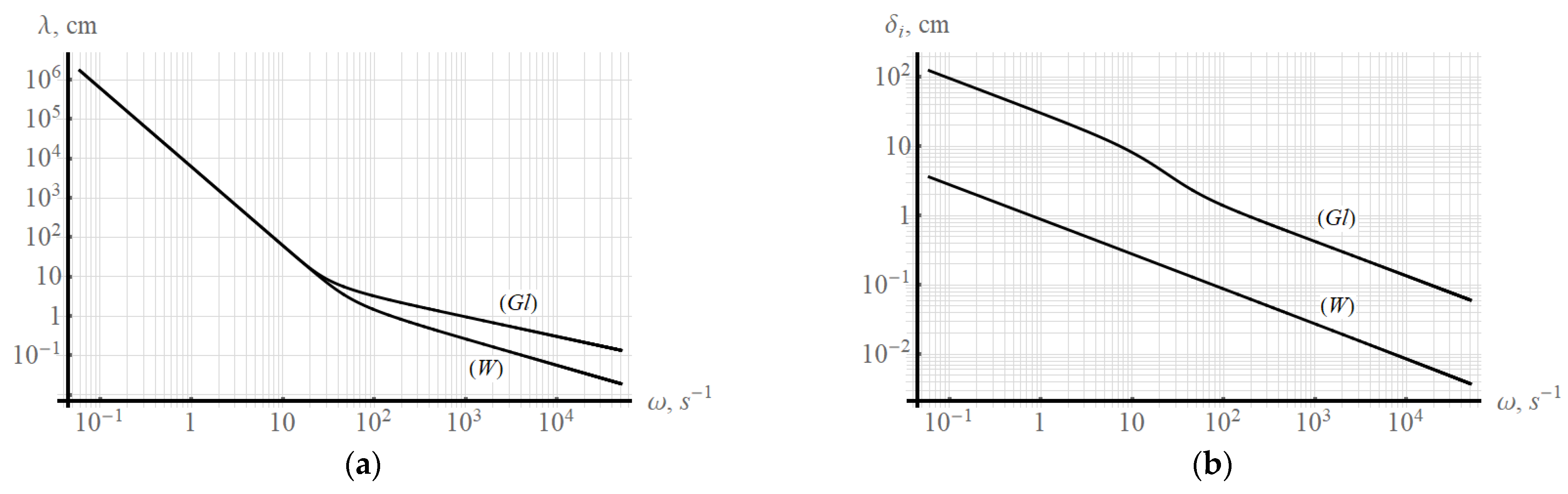
Figure 4 shows the dependence of the wavelength
on the frequency for the wave component (a) and the analog of the wavelength
on the frequency for the ligament component (b). The letter
indicates the dependencies for water and the letter
indicates the dependencies for glycerin.
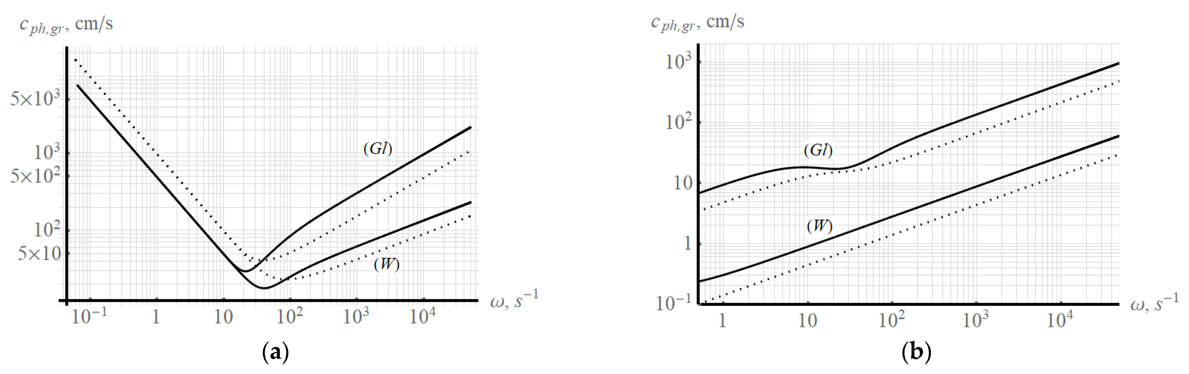
Figure 5 shows the dependences of the phase and group velocity on the frequency of periodic motion for the wave component of periodic motion (a) and the ligament associated with the wave component (b). The dependences are constructed for liquids with the parameters of water and glycerin.
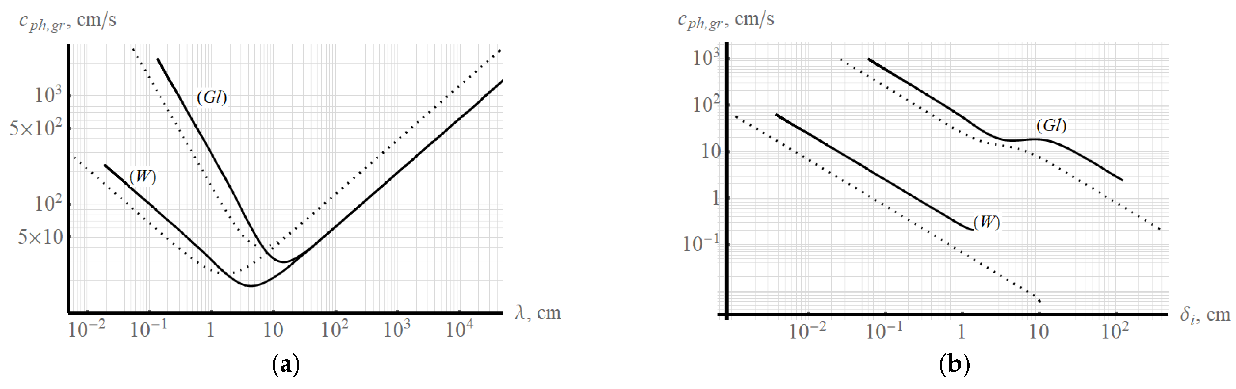
Figure 6 shows similar dependencies, but on the wavelength. There are several remarkable velocities in a viscous homogeneous liquid. The minimum group velocity and the velocity at which the group and phase velocities are compared. We show that the velocities are compared when the value of the phase velocity is minimal. The extremum condition for the phase velocity will be written as:
The ratio (62) leads us to equality:
The minimum value of the group velocity for a liquid with water parameters is and is achieved at frequency and wavelength . For a liquid with glycerin parameters, the corresponding values are as follows: at the frequency and wavelength . The minimum phase velocity for a liquid with water parameters is at the frequency and wavelength . For a liquid with glycerin parameters, the corresponding values are as follows: at frequency and wavelength .
The viscosity of the liquid affects the capillary wave motion. An increase in viscosity leads to an increase in the wavelength at a constant frequency in the region of capillary waves. As a consequence, the values of the phase and group velocity increase. The characteristic values of fluid velocities for the wave component of periodic motion increase with increasing viscosity and shift to the region of lower frequencies (longer wavelengths). Taking into account the viscosity in the model makes it possible to calculate, in addition to the wave component, the ligament component of periodic motion in a liquid.
5. Discussion
For the first time the theory of singular perturbations was used to describe the propagation of two-dimensional periodic perturbations over the surface of a viscous exponentially stratified incompressible fluid occupying the lower half-space. Calculations were performed in a single formulation in a wide frequency range, which includes the propagation of capillary, gravitational and internal waves. The system of equations, which includes the equations of continuity, momentum transfer and density profile with depth, replacing the equation of state, is solved together with physically justified kinematic and dynamic conditions on a free surface, taking into account the effect of surface tension. The theory of singular perturbations with respect to the compatibility condition was applied to study the propagation of infinitesimal harmonic flows with a positive definite frequency and a complex wavenumber, which considers spatial attenuation.
A complete set of solutions of the obtained dispersion relation for infinitesimal periodic perturbations includes two inseparable constituents of periodic flows. The theory of regular perturbations determines the parameters of gravitational-capillary or infra-low-frequency waves with a frequency lower than the buoyancy frequency.
The accompanying fine constituents that are ligaments are calculated by the methods of the theory of singular perturbations. The dispersion equation designed for infinitesimal periodic perturbations describes the relationship between the components of the wave vector in periodic flows in a wide frequency range which includes infra-low frequency, gravitational and capillary waves. The result, represented by length- frequency dependence, is convenient for experimental determination. The dependences of phase and group wave velocities on frequency and wavelength have also been obtained.
The dependences of phase and group velocities of regular perturbations (i.e., waves in water and glycerin) on frequency and wavelength have been represented in graphs. Wave properties are significantly modified during the transition through buoyancy frequency. The group velocity of wave propagation tends to zero and the phase one tends to infinity with the approximation of wave and buoyancy frequencies. Viscosity has a significant influence on short waves when their length becomes compared to or less than capillary scale .
The wave parameters are calculated in an actual homogeneous liquid in the limit of the buoyancy frequency as well as in a constant density approximation taking into account the compatibility conditions. These calculations correspond to the given results.
Singular solutions describe ligaments (i.e., thin currents accompanying waves in a viscous stratified or homogeneous liquid). To compare them we have shown the graphs of the dependence of the wavelength and scale of the ligaments on the wave frequency in a viscous homogeneous liquid. The sizes of the ligaments differ by several orders of magnitude at low frequencies. The dependences of the phase and group velocities of waves and ligaments on the frequency and wavelength are also given.
The application of the theory of singular perturbations makes it possible to design complete solutions of the dispersion equation and the system of fundamental equations without additional hypotheses and limitations of the type of boundary layer approximation [
33,
34].
The evolving approach admits the extrapolation to the investigation of three-dimensional periodic perturbations. In this case, propagating surface waves accompany several types of ligaments, as well as internal waves in the thickness of a continuously stratified liquid [
68,
69].
In general cases, both waves and ligaments continuously interact with each other and generate new groups of flow constituents [
75]. The influence of forcing together with the effects of nonlinearity and dissipation causes the evolution of the wave structure, which has different shapes at the phases of growth and attenuation.
In the low frequency range, the forcibly oscillating free surface of a stratified ocean can be a source of internal and inertial waves that transfer energy into the ocean. Internal waves, in turn, interact non-linearly with each other [
76], generating new wave groups and ligaments (i.e., accompanying flows that cause the observed modulation of the surface waves) [
77]).


