1. Introduction
Integro-Differential Equations, with their two parts Fredholm and Volterra, are considered a major factor in enriching modern applied mathematics, as their applications appear in many engineering sciences, including the theory of mechanics, elasticity, and many mathematical models with physical applications, as they are often written in the form of integral equations. In addition to some medical applications, including cancerous tumors. Here we mention the general form of nonlinear integro-differential equations of the type Volterra-Fredholm, (see [
1])
subject to the initial conditions
In the above equation, we assume that the
ℓth derivatives for
to
all are exists, also in Equation (
1) all the functions
and
are real functions and given, also
are real constants, while the two nonlinear parts
are the most difficult part in the problem, which makes the problem very interesting and makes the issue under discussion difficult in the process of finding a closed solution.
It has been shown that many physical or engineering phenomena are best represented mathematically by fractional calculus. In order to clarify some physical phenomena and study them more precisely and in more depth, the presence of fractional derivatives in the mathematical model gives more understanding and interpretation. The mathematical model that contains fractional derivatives is more accurate than the same model represented by integer order derivatives. We study here the fractional integro-differential equations, as they are effective models for explaining many engineering and physical phenomena. One of the advantages of using the fractional derivatives to model some phenomena is due to non-local property. As, it was shown [
2] the
order differential operator, where
n is an integer, also has a local property, on the other hand, where non-local properties appeared in the fractional order differential operators. This means that the study of a particular phenomenon, is not limited to its current situation, as much as we need to know many details about the previous history of the phenomenon, and this understanding comes through the intervention of fractional derivatives in the mathematical model. There are many studies that dealt with the subject of fractional derivatives, here we mention [
3,
4,
5,
6,
7], where a comprehensive study of the subject was presented, which made these studies a major reference for everyone who contributed to providing something new to the science of fractional derivatives. The study that was used in [
8] deals with an approximate solution, using Taylor series, to a fractional integro-differential equation that is very similar to the problem under discussion.
The main objective of this paper is to use Sumudu method to solve the general form of nonlinear Volterra-Fredholm integro-differential equation, that has the form
where in the above equation
represent the fractional derivative of
of order
. Sumudu presented for the first time the transformation called Sumudu in [
9,
10,
11,
12], in which all the basic properties were written, through which they were able to formulate some theorems that help in the treatment and finding solutions of differential equations of all kinds, ordinary, partial and integral equation. Sumudu transform is an effective transformation method used to solve many non-linear differential equations, which are often used as a mathematical model for many physical or engineering models. It is noteworthy that Sumudu transform have units preserving properties, and therefore can be used effectively to solve problems without resorting to the frequency domain, this is one of many strength points for Sumudu transform over Laplace transform, especially when dealing with physical sciences applications, where physical dimensions are important. In fact, the Sumudu transform which is itself linear, preserves linear functions, and hence in particular does not change units (see for instance Watugala [
9] or Belgacem et al. [
11]). Another advantage of using Sumudu over Laplace, is that, in solving differential equations that usually represents a model for many types of practical engineering models, where initial conditions have some singularities, Sumudu transform treats it accurately and effectively. Finally, when calculating inverse using Sumudu, we try to avoid tedious complex contour integration and its complications.
In [
13], the authors introduce some basic properties of the Sumudu transformation that will help to build and solve mathematical models. In [
14,
15], an effective method called Adomian decomposition method (ADM), which is dual to the Sumudu transformation, was used to solve the same system of nonlinear Volterra-Fredholm integro-differential Equation (
3). The Legendre collocation method was used in [
16], and Chebyshev wavelet in [
17], while the Tau approximations used in [
18] to solve nonlinear fractional integro-differential equation of the Volterra type, and the results are very promising. Other methods also used to solve similar problems as in [
8,
19,
20,
21,
22]. Previous studies related to the topic that the reader can refer to [
23,
24,
25]. In addition to the two references [
26,
27], where similar numerical methods were used, and the results were promising.
In this paper, we will first provide all the definitions or theorems we need related to the Sumudu method, and then formulate the general solution to Equation (
3) using the proposed method that we call, Sumudu Adomian decomposition method (SADM). This method is more effective than other methods, like Legendre collocation method that will be used for comparison purposes in the last section, because it gives an accurate approximate solutions to the integral equations with fractional derivatives to a large extent. It is worth noting that one of the benefits of the method under consideration is that it reduce the computational time and volume of work. We would like to point out that in using other methods, to solve the problem as it appeared in Equation (
3), it requires finding the solution at each change of the value of the constant
. On the contrary, when using the method (SADM) which gives the answer in terms of the constant
, and thus it is easy to calculate the solution at different values of
, and no need to solve the problem again, it only requires substituting that value for
in the computed solution. The most important part in Equation (
3) is the left-hand side known as the fractional differential operator, denoted as
, which describes the fractional derivatives of order
. If the value of
is an integer, then the question under consideration goes back to the ordinary derivatives, which is a special case of the study in this paper. Therefore, considering
as fractional positive number makes Equation (
3) a generalization of the work [
36].
The main presentation of the contents of this research came as follows: In
Section 2, we briefly review some of the main concepts related to the theorem of fractional calculus, in addition to briefly introducing some theorems related to the Sumudu transformation, which will be used to solve the problem under consideration. In
Section 3, we apply the Sumudu transformation, by first substituting the nonlinear term by their Adomian’s polynomials, and writing the general solution to the problem as given in Equation (
3) in the form of a series in terms of the parameter
. Some results are stated in regards to existence, uniqueness, and the maximum absolute error of the truncated series solution have been proved in
Section 4. Finally in
Section 5, the credibility of the method was confirmed by experimenting with three different examples. The results were presented in the form of tables and graphics that showed the accuracy and effectiveness of the method. The paper ends with some concluding remarks.
2. Basic of Fractional Calculus
In order to identify the properties of fractional calculus, we present in this section some definitions and studies that we need to write the solution to the problem under consideration. There are many definitions that were presented in previous years for fractional derivatives, and here we will use the Riemann-Liouville definition, and thus Riemann-Liouville is defined for fractional integral operator
in the following form [
28].
Definition 1. Let . The operator , defined on the usual Lebesque space byfor , is called the Riemann-Liouville fractional integral operator of order α. Properties of the operator
can be found in [
6], we mention the following: For
and
exists for almost every .
When using the Riemann-Liouville definition to treat problems that represent the mathematical model of some physical phenomena, some shortcomings appear in the Riemann-Liouville definition. Thus we will use the improved Caputo definition for the fractional differentiation operator , as follows
Definition 2. Caputo introduces derivatives of fractional orders of a function as follows While we present here two basic properties of fractional calculus.
Lemma 1. If , and , then , and The reason for adopting Caputo definition for solving fractional differential equations, is that, in order to obtain a unique and exact solution to the equation, we need to specify additional initial conditions for the fractional equation. Caputo definition has been well received for this purpose. The Caputo definition is widely acclaimed because it makes it possible to define initial conditions that relate to the integer derivatives of the derived functions in the models considered. It should be noted here that there are many studies that dealt in detail with the study of the geometric interpretation of fractional derivatives, see for example [
29].
Definition 3. Caputo defines the fractional derivatives order α, such that for m be an integer that is the smallest to exceeds α, we have For further study on the properties and adjectives of Caputo definition in relation to derivatives and fractional integrals, the reader can refer to the following resources [
29].
Watugala [
9,
10] introduced a new transformation known as Sumudu transform, that used to solve differential equations with Engineering applications.
Definition 4. Sumudu transform over the following set of functionsis defined as, for , we havewhere u is a parameter and it may be real or complex that is independent of t. The inversion formula for Sumudu transform is given by It has been shown in [
30], that the Laplace and Sumudu transformations are equivalent, but using one of them may be easier in terms of calculations than the other, especially when solving intgro-differential equations, and in fact this is why we use the Sumudu transform to solve the same problem in [
14]. Given an initial
, its Laplace transform
can be transformed into the Sumudu transform
of
f by means of
Every property proved of the Laplace transform may routinely be turned into a corresponding property of the Sumudu transform. In [
11,
30], the researchers presented a sufficient and extensive study on the Sumudu transformation, where many of the basic properties and theories related to the Sumudu transformation were presented, and here we mention only what we need.
Theorem 1 ([
30])
. Let be a function, and let’s denote the Sumudu transformation of to be , and the following are satisfied The following fact is often used to find solutions to differential equations with fractional derivatives.
Lemma 2 ([
31])
. The Sumudu transform of the fractional derivative introduced by Caputo is given by 3. Implementation of Sumudu Decomposition Method
In order to present the Sumudu Adomian decomposition (SAD) used in this paper, we first assume that the problem, as it appeared in the Equations (
1) and (
2), has a unique and smooth solution to a sufficient degree to deal with it [
32]. Before starting to find an approximate solution to problem (
3), using the proposed method (SAD), we assume that the unknown function
is differentiable several times and the solution we are looking for is unique. We apply the Sumudu transformation to the five sides in Equation (
3), and write it as
Using the result of Lemma 2, after replacing the value of
, in the above equation, we obtain
Solve for
, we get
where
. Now, following [
1,
33,
34]. The Sumudu decomposition method consists of decomposing the unknown function
of any equation into a sum of an infinite number of components defined by the decomposition series:
where the components
are to be determined in a recursive manner. To calculate the components of the solution in a recursive way, we define the nonlinear functions
, by a series of polynomials set as:
where the symbols
, depends on
, and named as Adomian’s polynomials that represent the non-linear functions in the given integral equation, and the special formula set by Adomian [
33,
34], or Wazwaz [
35] is used to find these polynomials. Substituting these infinite series (
7)–(
8)
, we obtain
The process of forming the recursive equations for the series solution depends mainly on choosing the first term
in the series to consist of all the terms that came from the initial conditions, or from the term related to the source term
, i.e.,
As for calculating the other terms for
, we calculate each term in terms of the previous one’s and alternately, so for
, we have
As a result, the components
are identified by applying inverse Sumudu transform of the above equations, to obtain
and, for
, we arrive at
In this way, a sufficient number of terms for the series approximate solution can be calculated. It should be noted here that we only few terms are needed to get a fairly accurate solution. In many cases, the exact solution to the problem can be known, especially if the value of
is an integer [
1]. The partial sum of the approximate solution, that represent the first
n terms is given by
. The process of calculating terms of the series solution depends mainly on the nature of the shape of the first term in Equation (
9), especially when finding the inverse, it becomes difficult whenever there are many terms in Equation (
9). Wazwaz [
35] adopted a new method when he faced the same problem for applying Adomian decomposition method, he proposed dividing the first term appearing in Equation (
9) into two (or more) parts, the first part
is taking to be
, which is easy to calculate its inverse. Then for the second part, he proposed
, in this way, the rest of the terms were calculated easily. We will follow the same method suggested as Wazwaz, as we will see in the illustrative examples.
5. Illustrative Examples
In order to assess the advantages of the proposed method (Sumudu Adomian decomposition) over Adomian Decomposition method [
14], in terms of accuracy and efficiency for solving fractional integro-differential equations, we have applied the method to two different examples, with known exact solutions at some values of
. The computations associated with the examples were performed using Mathematica.
Example 1. Consider the following nonlinear fractional integro-differential equation [17]where , and . Applying the Sumudu transform to both sides of Equation (
12). For the left hand side part
we use the initial condition together with Lemma 2, while for the first three terms on the right hand side we use the fact that
By presenting some simple but annoying calculations in which there is no need to explain them here, we came to the following
Substituting the decomposition series (
7) for
, and the series
for the nonlinear term
, we have
Because we need to calculate a few terms from the solution series, then we need to know the first
Adomian polynomials, as
, and so on. The modified decomposition technique introduces the use of the recursive relation
and,
In general, we take the
term to be
Take the inverse Sumudu transform of both sides of
, yields
So we can simplify
appeared in Equation (
14) as
Take the Sumudu inverse
of both sides, we obtain the result
To obtain the inverse Sumudu of
from (
15), we use Mathematica to avoid a lengthy calculations. The approximate solution is given by
. When
, then
which is the exact solution. The value of
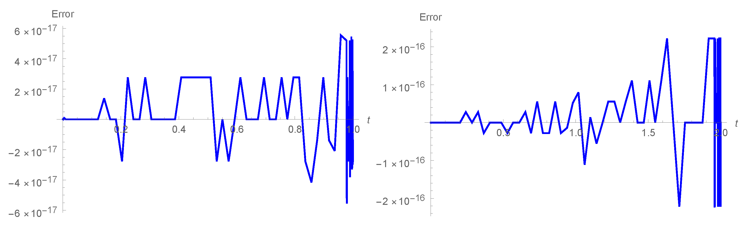
is the only case for which we know the exact solution, and our approximate solution is in excellent agreement with the exact values as shown in
Figure 1, where we drew the absolute error between the exact and the approximate solutions when
, and the solution calculated by the method for two different periods. The results in
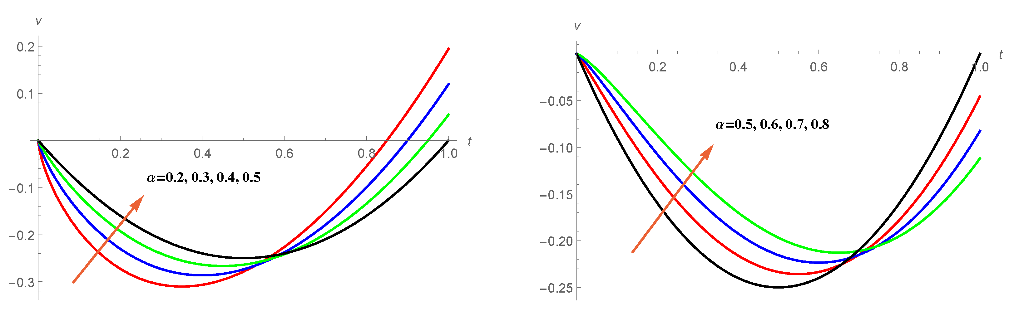
Figure 1 showed the effectiveness of the method. Thus we have drawn the solution at other values of
as in
Figure 2, and we can conclude from the drawings that the solution at different values of
has the same behavior. Computational cost of the numerical scheme varying the number of iterations, in this example only two iterations are needed in a time of 1.32 s.
In many cases the modified scheme proposed by Wazwaz [
35] avoids the unnecessary computations for Adomian polynomials, also, no need to calculate several terms of the series solution, as the computation will be reduced very considerably by using the modified scheme. The next example we present a fractional linear Volterra-Fredholm integro-differential equation, which represents the general formula for the problem under consideration as stated in Equation (
1), and the modified scheme will be used.
Example 2. Consider the fractional linear Voltera-Fredholm integro-differential equation of order α, where .when
and the initial condition is
, Equation (
17) has exact solution
. Imitating what came at the beginning of the solution to the first example, where Sumudu was taken to both sides and some relations related to Sumudu transform were used, for
we arrive at
Substituting the decomposition series (
7) for
on both sides of the above equation, while it should be noted that there are no non-linear terms inside the kernels, as the equation under study is linear, and therefore we do not need Adomian polynomials. So, we get
The modified decomposition technique introduces the use of the first two iterations as
and,
In Equations (
19) and (
20), take the inverse Sumudu of both sides we get
, and
. Since all remaining terms
depends on
, so we have
for all
. Therefore, the obtained solution is
, which is the exact solution.
Example 3. Now we present a nonlinear example of a special type of Volterra integro-differential equation of the form Equations of Volterra types appear a lot in engineering applications, especially in the subject of glass forming process. For Equation (
21) is known that the exact solution when
, is
[
36].
We will find the approximate solution as a function both
t and
, and use the obtained solution to compare it with the exact solution when
. In addition to that, the accuracy of the solution will be compared with the results in [
36]. To start, we take Sumudu transform on both sides of Equation (
21) to get
The method is to substitute what was stated in Equation (
7) on the left side of the above equation, while we replace the non-linear term that came in the form of the product of
with its first derivative
in the form of Adomian polynomials, as
. Because we will be satisfied with finding the first 6 terms of the solution series in Equation (
7), we need to calculate only the first 5 terms of the Adomian polynomials, the first 4 came as follows:
,
,
,
. Similarly
with more terms. Therefore, after the appropriate substitutions, as mentioned above, Equation (
22) becomes
After comparing the two sides, we get the value of the first term from the left side
to be
, after taking the inverse, we get that the value of
. The remaining alternating terms are given by the following relationship
After taking the inverse of both sides, we get
After substituting the values of
into Equation (
24), and after easy arithmetic operations, we calculate from the approximate series solution (
7) the first 6 terms, and write the approximate solution as follows
where
and
For the purposes of comparison with the exact solution
, we write the approximate solution when the value of
in the following form
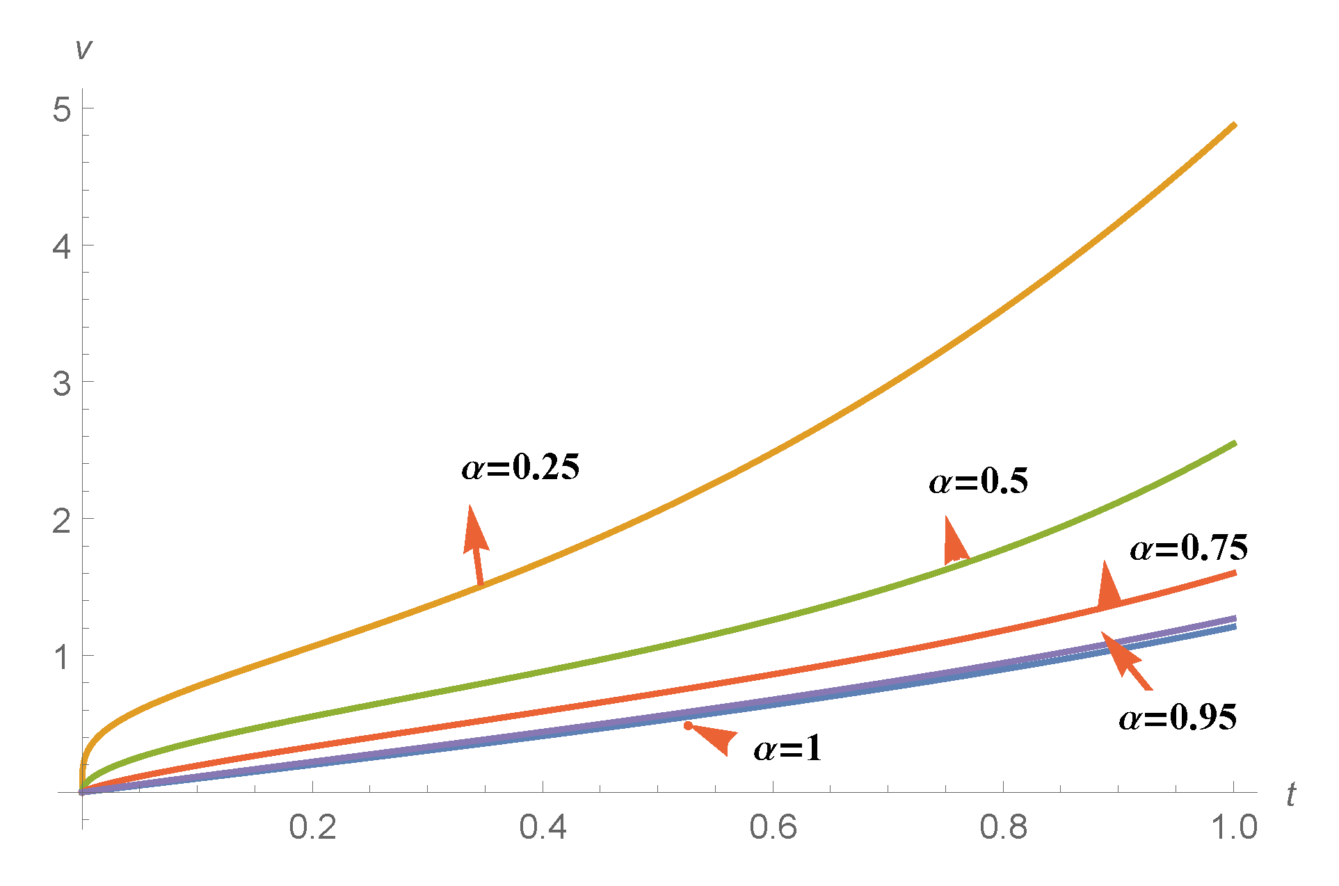
We used the approximate solution in Equation (
25) and plotted the solution as in
Figure 3 for several different values of
starting from
till
. Looking at the figure, we notice that the behavior of the solution seems to be the same, especially the closer we get to the exact solution when
. As we mentioned earlier, the equation in this example has exact solution only when the value of
is 1, so in
Table 1, we calculated the approximate solution in Equation (
25) when
is equal to 1 at several values of the variable
t. The results were compared with the Laplace Adomian Decomposition method, which was used in [
36], to solve the same example. The results showed that our method is slightly better than the one in [
36].
We can observe the following from the results of the above three examples: (a) the convergence of the method when the number of iterations increases; (b) an estimate of the rate of convergence and of the computational cost of the method; (c) a comparison with other numerical schemes proposed in the literature, like Legendre collocation method; (e) a detailed examination of the convergence in terms of its simplicity, implementation and high accuracy; (f) when the fractional derivative tends to positive integer, then the approximate solution continuously tends to the exact solution.


