Article

Dynamic Behaviors of an Obligate Commensal Symbiosis Model with Crowley–Martin Functional Responses

College of Mathematics and Physics, Ningde Normal University, Ningde 352000, China
*
Author to whom correspondence should be addressed.
Axioms 2022, 11(6), 298; https://doi.org/10.3390/axioms11060298
Submission received: 2 June 2022 / Revised: 13 June 2022 / Accepted: 15 June 2022 / Published: 20 June 2022
(This article belongs to the Special Issue Advances in Applied Mathematical Modelling)

Abstract

:
A two species obligate commensal symbiosis model with Crowley–Martin functional response was proposed and studied in this paper. For an autonomous case, local and global dynamic behaviors of the system were investigated, respectively. The conditions that ensure the existence of the positive equilibrium is coincidentla to the conditions of global stability of a positive equilibrium. For nonautonomous cases, persistent and extinction properties of the system are investigated.
JEL Classification:
92D25; 34D20

1. Introduction

During the last decades, many scholars investigated the dynamic behaviors of the commensalism model; see [1,2,3,4,5,6,7,8,9,10,11,12,13,14,15,16,17,18,19,20,21,22,23,24,25,26,27,28,29,30,31,32,33,34,35,36,37] and the references cited therein. Topics such as the stability of the system [1,2,3,4,5,6,7,8,9,10,37], the existence of periodic solution or almost periodic solution [11,15,25,36], the influence of harvesting [1,2,3,12,13,14,26,27,28], the influence of stage structure ([16]), the influence of Allee effect [9,17,18,19,20,24,32,33], the bifurcation phenomenon of the system [9,29,32,33], the influence of feedback control [8,23], the persistent property of the system [34,35,37], the influence of commensalism to the ecological network [6,7], and the influence of stochastic disturbance [5] were extensively investigated by many scholars. However, the commensalism model is not well studied in the sense that, to this day, still a few works on commensal symbiosis model with one party cannot survive independently [34,35,36,37].
Yang et al. [34] proposed the following non-autonomous obligate commensalism model:
x ˙ = x a 1 ( t ) b 1 ( t ) x + c 1 ( t ) y , y ˙ = y a 2 ( t ) b 2 ( t ) y .
where a 1 ( t ) , a 2 ( t ) , b 1 ( t ) , c 1 ( t ) , and b 2 ( t ) are all continuous functions bounded above and below by positive constants. They paid attention to the persistent, extinction, and stability of the system. Chen et al. [35,36] proposed and studied a discrete commensal symbiosis model.
Recently, stimulated by the concept of functional response of the predator prey system, Wu et al. [37] proposed the following obligate commensalism model with ratio-dependent functional responses.
d x d t = x a 1 b 1 x + c 1 y x + y , d y d t = y ( a 2 b 2 y ) .
They provided a thoroughly investigation about the dynamic behaviors of the system (2).
As for as functional response is considered, there are many type functional responses on predator prey system. In his pioneering work, Holling [38] argued that, in the predator prey system, functional response should take into consideration; from then on, numerous works (see, for example, [39,40]) were been performed on Holling type II and III functional response. Noting that the predators hunt for food resources and as a consequence they have to share food or involve intra-specific competition, to describe this phenomenon, a ratio-dependent functional response [41] was introduced, and the functional response is dependent on both predator and prey species instead of only prey dependent functional response. However, scholars argued that the predator prey model with a ratio-dependent functional response has curious dynamic behaviors; to overcome the drawback of the system, the Beddition–DeAngelis functional response, which can be seen as the generalization of the ratio-dependent and Holling II functional response functional response [42], was introduced. In 1989, Crowley and Martin [43] proposed a functional response, which is similar to the Beddington–DeAngelis response function, but it includes one more term explaining mutual interferences of predators at the high density of its prey. Many scholars performed works on predator prey system with Crowley–Martin functional responses; see [44] and the references cited therein. The Crowley–Martin functional response can be seen as the generalization of the Holling II functional response, ratio-dependent functional response, and Beddition–DeAngelis functional response. Noting that to this day, still no scholars propose and study the commensalism model with Crowley-Martin functional response. This motivated us to propose the following model.
d x d t = x a 1 b 1 x + c 1 y d 1 + e 1 x + f 1 y + g 1 x y , d y d t = y ( a 2 b 2 y ) .
Throughout this paper, we assume that ( H 1 ) or ( H 2 ) hold; here, ( H 1 ) a i , b i , i = 1 , 2 and c 1 , d 1 , e 1 , f 1 , g 1 are all positive constants. ( H 2 ) a i ( t ) , b i ( t ) , i = 1 , 2 and c 1 ( t ) , d 1 ( t ) , e 1 ( t ) , f 1 ( t ) , g 1 ( t ) are all continuous functions bounded above and below by some positive constants.
The aim of this paper is to provide a thorough investigation about the dynamic behaviors of the system (3). For the autonomous case, we will investigate the local stability property of the equilibria in the next section. The global stability property is then investigated in Section 3. For the nonautonomous case, we investigate persistent and extinction properties in Section 4. Some numeric simulations are carried out in Section 5 to show the feasibility of our results. We end this paper by a brief discussion.

2. The Existence and Local Stability of the Equilibria

Now let us consider the autonomous case; i.e., assume that ( H 1 ) holds.
Concerned with the existence of the equilibria, we have the following result.
Theorem 1.
System (3) always admits the boundary equilibrium A 0 ( 0 , 0 ) and A 1 0 , a 2 b 2 . Assume further that the inequality of the follow:
c 1 > a 1 f 1 + a 1 d 1 b 2 a 2
holds; then, system (3) admits a unique positive equilibrium A 2 ( x * , y * ) , where the following is the case.
x * = A 2 + A 2 2 4 A 1 A 3 2 A 1 , y * = a 2 b 2 ,
Here, we have the following.
A 1 = a 2 b 1 g 1 + b 1 b 2 e 1 > 0 , A 2 = a 1 a 2 g 1 + a 1 b 2 e 1 + a 2 b 1 f 1 + b 1 b 2 d 1 , A 3 = a 1 f 1 a 2 + a 1 d 1 b 2 c 1 a 2 < 0 .
Proof. 
The equilibria of system (3) is determined by the following system.
x a 1 b 1 x + c 1 y d 1 + e 1 x + f 1 y + g 1 x y = 0 , y ( a 2 b 2 y ) = 0 .
System (3) always admits the boundary equilibrium A 0 ( 0 , 0 ) and A 1 0 , a 2 b 2 . Now, let us consider the positive equilibrium. From the second equation of (4), the following immediately follows.
y = a 2 b 2 .
Substituting (8) into the first equation of (4) and simplify, we finally obtain the following:
A 1 x 2 + A 2 x + A 3 = 0 ,
where A i , i = 1 , 2 , 3 are defined by (6). Now let us consider the following function.
F ( x ) = A 1 x 2 + A 2 x + A 3 ,
Noting that A 1 > 0 implies that F ( ) = F ( + ) = + , A 3 < 0 leads to F ( 0 ) = A 3 < 0 , form the continuity of function F, and fact F has at most two real solutions where F has a unique solution on ( 0 , + ) . Hence, Equation (9) has a unique positive solution.
x * = A 2 + A 2 2 4 A 1 A 3 2 A 1 .
Consequently, system (3) has a unique positive solution A 2 ( x * , y * ) .
This ends the proof of Theorem 1. □
Obviously, A 2 x * , y * satisfies the following equation.
a 1 b 1 x * + c 1 y * d 1 + e 1 x * + f 1 y * + g 1 x * y * = 0 , a 2 b 2 y * = 0 .
Concerned with the local stability property of the above three equilibria, we have the following.
Theorem 2.
A 0 ( 0 , 0 ) is unstable; A 1 0 , a 2 b 2 is unstable if c 1 > a 1 f 1 + a 1 d 1 b 2 a 2 holds and locally stable if c 1 < a 1 f 1 + a 1 d 1 b 2 a 2 holds; if A 2 x * , y * exists, it is locally stable.
Proof. 
The Jacobian matrix of system (3) is calculated as follows:
J ( x , y ) = A 11 A 12 0 2 b 2 y + a 2 ,
where the following is the case.
A 11 = a 1 b 1 x + c 1 y d 1 + e 1 x + f 1 y + g 1 x y + x b 1 c 1 y ( g 1 y + e 1 ) ( d 1 + e 1 x + f 1 y + g 1 x y ) 2 , A 12 = x c 1 ( e 1 x + d 1 ) ( d 1 + e 1 x + f 1 y + g 1 x y ) 2 .
Then, the Jacobian matrix of the system (3) about equilibrium A 0 ( 0 , 0 ) is given by the following.
a 1 0 0 a 2 .
The corresponding eigenvalues are λ 1 = a 1 < 0 , λ 2 = a 2 > 0 . Hence, A 0 ( 0 , 0 ) is unstable.
Then, the Jacobian matrix of the system (3) about equilibrium A 1 ( 0 , a 2 b 2 ) is given by the following.
a 1 a 2 f 1 + a 1 b 2 d 1 a 2 c 1 a 2 f 1 + b 2 d 1 0 0 a 2 .
The corresponding eigenvalues are λ 1 = a 1 a 2 f 1 + a 1 b 2 d 1 a 2 c 1 a 2 f 1 + b 2 d 1 , λ 2 = a 2 < 0 . Obviously, if c 1 < a 1 f 1 + a 1 d 1 b 2 a 2 , then λ 1 < 0 , in this case, A 1 ( 0 , r 2 a 22 ) is locally stable; A 1 ( 0 , r 2 a 22 ) is unstable if c 1 > a 1 f 1 + a 1 d 1 b 2 a 2 .
By using (12), the Jacobian matrix about the positive equilibrium A 2 is given by the following.
x * b 1 + c 1 y * ( g 1 y * + e 1 ) ( d 1 + e 1 x * + f 1 y * + g 1 x * y * ) 2 x * c 1 ( e 1 x * + d 1 ) ( d 1 + e 1 x * + f 1 y * + g 1 x * y * ) 2 0 b 2 y * .
The eigenvalues of the above matrix are λ 1 = x * b 1 + c 1 y * ( g 1 y * + e 1 ) ( d 1 + e 1 x * + f 1 y * + g 1 x * y * ) 2 < 0 , λ 2 = b 2 y * < 0 . Hence, A 2 ( x * , y * ) is locally stable.
This ends the proof of Theorem 2. □

3. Global Stability of the Equilibria

We also assume that ( H 1 ) holds in this section.
We will investigate the global stability property of the equilibria in this section.
Theorem 3.
Assume that c 1 < a 1 f 1 + a 1 d 1 b 2 a 2 holds; then, A 1 0 , a 2 b 2 is globally attractive.
Proof. 
Inequality c 1 < a 1 f 1 + a 1 d 1 b 2 a 2 is equivalent to the following.
c 1 a 2 b 2 < a 1 f 1 a 2 b 2 + a 1 d 1 .
The above inequality also equivalent to the following.
a 1 > c 1 a 2 b 2 f 1 a 2 b 2 + d 1 .
From (19), forsmall enough ε > 0 , the following inequality:
a 1 > c 1 ( a 2 b 2 + ε ) f 1 ( a 2 b 2 + ε ) + d 1
holds.
Noting that the second equation of (3) takes the following form.
d y d t = y ( a 2 b 2 y ) .
System (18) has a unique globally attractive positive equilibrium y * = a 2 b 2 .
lim t + y ( t ) = y * .
For ε > 0 that is small enough, which satisfies (20), it follows from (22) that there exists a large enough T 1 > 0 such that the following is the case.
y ( t ) < a 2 b 2 + ε .
Now let us consider the following function.
F ( y ) = c 1 y d 1 + e 1 x + f 1 y + g 1 x y ,
Note the following.
d F ( y ) d y = c 1 ( e 1 x + d 1 ) ( d 1 + e 1 x + f 1 y + g 1 x y ) 2 > 0 .
Hence, F ( y ) is the strictly increasing function of y; hence, from the first equation of (3) and (23), for t > T 1 , we have the following.
d x d t = x a 1 b 1 x + c 1 y d 1 + e 1 x + f 1 y + g 1 x y x a 1 + c 1 y d 1 + f 1 y x a 1 + c 1 a 2 b 2 + ε d 1 + f 1 a 2 b 2 + ε ,
Hence, the following is the case.
x ( t ) x ( T 1 ) exp a 1 + c 1 a 2 b 2 + ε d 1 + f 1 a 2 b 2 + ε ( t T 1 ) 0 as t + .
(22) and (27) show that A 1 ( 0 , a 2 b 2 ) is globally attractive. This ends the proof of Theorem 3. □
Theorem 4.
Assume that c 1 > a 1 f 1 + a 1 d 1 b 2 a 2 holds; then, A 2 x * , y * is globally stable.
Proof. 
In the proof of Theorem 3, we showed that lim t + y ( t ) = a 2 b 2 . That is, for any ε > 0 that is small enough, there exists T > 0 such that for all t > T 1 , the following is the case.
y * ε < y ( t ) < y * + ε for all t > T 1 .
From the first equation of system (3), we have the following.
d x d t x a 1 b 1 x + c 1 f 1 ,
Thus, the following is the case.
lim sup t + x ( t ) c 1 f 1 a 1 b 1 .
That is, there exists a T 2 > T 1 such that the following is the case.
x ( t ) < c 1 f 1 a 1 b 1 + ε for all t > T 2 .
Let D = { ( x , y ) | R + 2 : x < c 1 f 1 a 1 b 1 + ε , y < a 2 b 2 + ε . } . Then, every solution of system (3) starting in R + 2 is uniformly bounded on D. Moreover, from Theorem 2, A 0 ( 0 , 0 ) and A 1 ( 0 , a 2 b 2 ) are all unstable, and the unique positive equilibrium A 2 ( x * , y * ) is locally stable. To ensure A 2 ( x * , y * ) is globally stable in the above area, we consider Dulac function u ( x , y ) = x 1 y 1 ; then, we have the following:
( u P ) x + ( u Q ) y = b 1 y b 2 x c 1 ( g 1 y + e 1 ) ( d 1 + e 1 x + f 1 y + g 1 x y ) 2 < 0 ,
where P ( x , y ) = x a 1 b 1 x + c 1 y d 1 + e 1 x + f 1 y + g 1 x y , Q ( x , y ) = y ( a 2 b 2 y ) . By Dulac Theorem [31], there is no closed orbit in area D. Thus, A 2 ( x * , y * ) is globally asymptotically stable.
This completes the proof of Theorem 4. □

4. Nonautonomous Case

Now let us consider the following system:
d x d t = x a 1 ( t ) b 1 ( t ) x + c 1 ( t ) y d 1 ( t ) + e 1 ( t ) x + f 1 ( t ) y + g 1 ( t ) x y , d y d t = y ( a 2 ( t ) b 2 ( t ) y ) ,
where a i ( t ) , b i ( t ) , c 1 ( t ) , i = 1 , 2 are all continuous functions bounded above and below by positive constants. For the rest of the paper, for a bounded continuous function g defined on R, let g L and g M be defined as follows.
g L = inf t R g ( t ) , g M = sup t R g ( t ) .
As for as system (33) is concerned, the most important thing is to find out the conditions that ensure the permanence of the system, which means that the species could be coexist in the long run. Moreover, in today’s society, more and more species are rapidly reduced or even extinct; hence, it is also important to investigate the extinction property of the system. The aim of this section is to investigate the extinction and persistent property of the system.
Concerned with the extinction of the first species, we have the following result.
Theorem 5.
Assume the following:
a 1 L > c 1 M M 2 d 1 L + f 1 L m 2
holds, where M 2 , m 2 are defined in (39) and (41), respectively; then, we have the following:
lim t + x ( t ) = 0 .
i.e., the first species will be driven to extinction.
Proof. 
It follows from (35) that for small enough ε > 0 , without a loss of generality, assume that ε < 1 2 m 2 , and the following inequality holds.
a 1 L > c 1 M ( M 2 + ε ) d 1 L + f 1 L ( m 2 ε )
Let ( x ( t ) , y ( t ) ) be any solution of system (33) with initial conditions x ( 0 ) > 0 , y ( 0 ) > 0 .
From the second equation of system (33), we have the following.
y ˙ ( t ) y a 2 M b 2 L y ,
Thus, the following is the case.
lim sup t + y ( t ) a 2 M b 2 L = def M 2 .
From the second equation of system (33), we have the following.
y ˙ ( t ) y a 2 L b 2 M y ,
Thus, the following is the case.
lim inf t + y ( t ) a 2 L b 2 M = def m 2 .
For any ε > 0 that is small enough such that inequality (37) holds, it follows from (39) and (41) that there exists a T > 0 such that the following is the case.
m 2 ε < y ( t ) < M 2 + ε for all t > T .
For t > T , from the first equation of system (33), the following is the case.
x ˙ ( t ) = x a 1 ( t ) b 1 ( t ) x + c 1 ( t ) y d 1 ( t ) + e 1 ( t ) x + f 1 ( t ) y + g 1 ( t ) x y x a 1 ( t ) b 1 ( t ) x + c 1 ( t ) y d 1 ( t ) + f 1 ( t ) y x a 1 L b 1 L x + c 1 M ( M 2 + ε ) d 1 L + f 1 L ( m 2 ε ) .
Thus, the following is the case.
x ( t ) x ( T ) exp a 1 L b 1 L x + c 1 M ( M 2 + ε ) d 1 L + f 1 L ( m 2 ε ) ( t T ) 0 as t + .
This ends the proof of Theorem 5. □
Lemma 1.
Assume that c d > a ; then, the following system:
d y d t = y a b y + c e y + d
admits a unique positive equilibrium x * , which is globally attractive, where a , b , c , d , and e are all positive constants.
Proof. 
With some minor revision, the proof of Lemma 1 is similar to the proof of Lemma 3.1 in [37], and we omit the details here. □
Concerned with the persistent property of the system, we have the following result.
Theorem 6.
Assume the following:
a 1 M < c 1 L m 2 d 1 M + f 1 M M 2
holds, where M 2 , m 2 are defined in (39) and (41), respectively; then, system (33) is permanent.
Proof. 
It follows from (46) that for small enough ε > 0 , without loss of generality, assume that ε < 1 2 m 2 ; the following inequality holds.
a 1 M < c 1 L ( m 2 ε ) d 1 M + f 1 M ( M 2 + ε ) .
Let ( x ( t ) , y ( t ) ) be any solution of system (33) with initial conditions x ( 0 ) > 0 , y ( 0 ) > 0 . similarly to the analysis of (37)–(40), for any ε > 0 small enough such that inequality (47) holds; there exists a T > 0 such that the following is the case.
m 2 ε < y ( t ) < M 2 + ε for all t > T .
For t > T , from the first equation of system (33), the following is the case.
x ˙ ( t ) = x a 1 ( t ) b 1 ( t ) x + c 1 ( t ) y d 1 ( t ) + e 1 ( t ) x + f 1 ( t ) y + g 1 ( t ) x y x a 1 L b 1 L x + c 1 M f 1 L .
Hence, the following holds
lim sup t + x ( t ) c 1 M f 1 L a 1 L b 1 L .
From the first equation of system (33), the following is the case.
x ˙ ( t ) x a 1 M b 1 M x + c 1 L ( m 2 ε ) d 1 M + e 1 M x + f 1 M ( M 2 + ε ) + g 1 M x ( M 2 + ε ) = x a 1 M b 1 M x + c 1 L ( m 2 ε ) d 1 M + f 1 M ( M 2 + ε ) + ( e 1 M + g 1 M ( M 2 + ε ) ) x .
Now, let us consider the following equation.
w ˙ ( t ) = w a 1 M b 1 M w + c 1 L ( m 2 ε ) d 1 M + f 1 M ( M 2 + ε ) + ( e 1 M + g 1 M ( M 2 + ε ) ) w .
Since the following is the case:
c 1 L ( m 2 ε ) d 1 M + f 1 M ( M 2 + ε ) > a 1 M ,
it follows from Lemma 1 that (52) admits a unique positive equilibrium w ε * , which is globally stable. Thus, by the comparison theorem of the differential equation, one has the following:
lim inf t + x ( t ) w ε * ε .
and it immediately follows from (48), (50) and (54) that system (3) is permanent. This ends the proof of Theorem 6. □

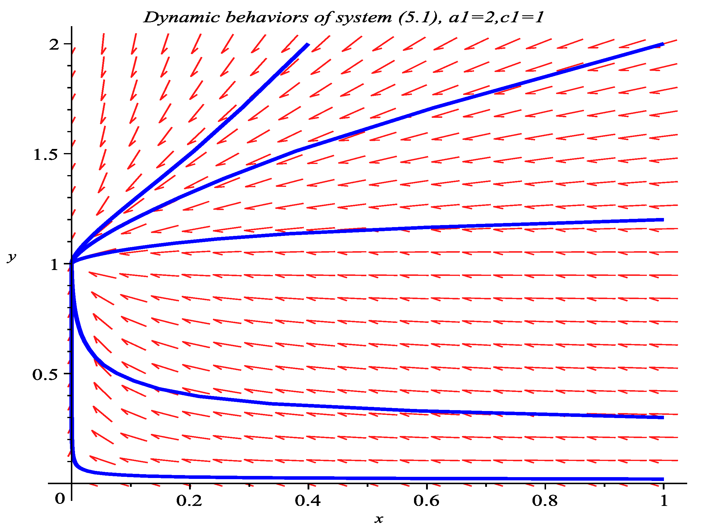
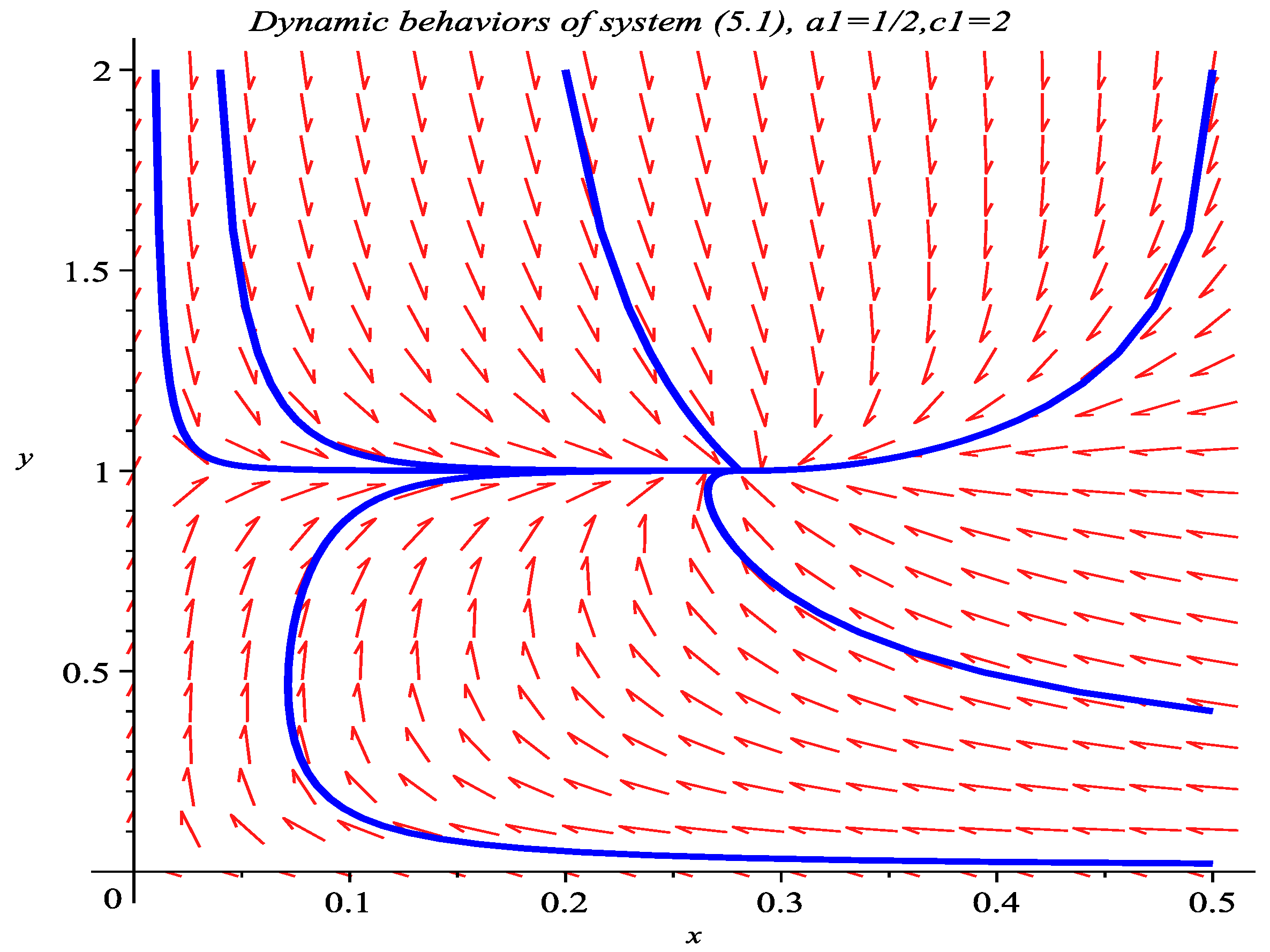
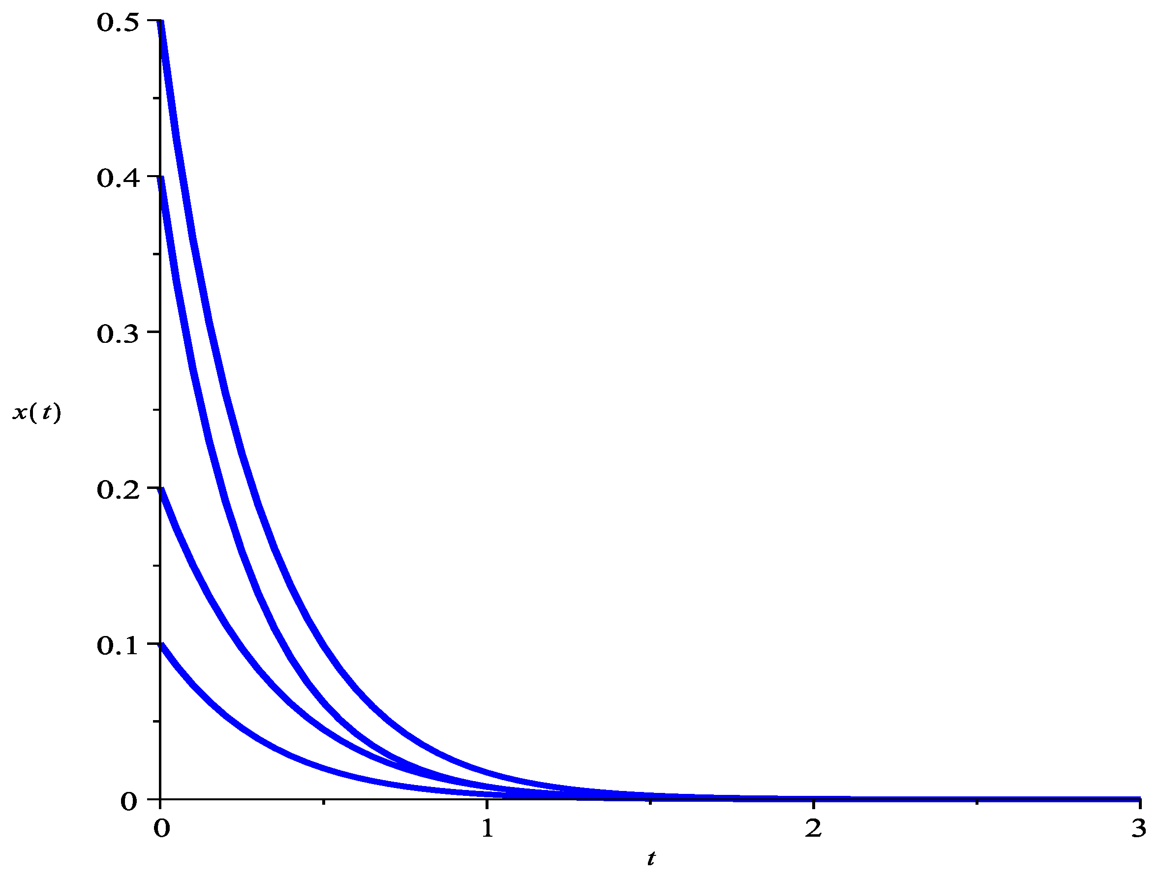
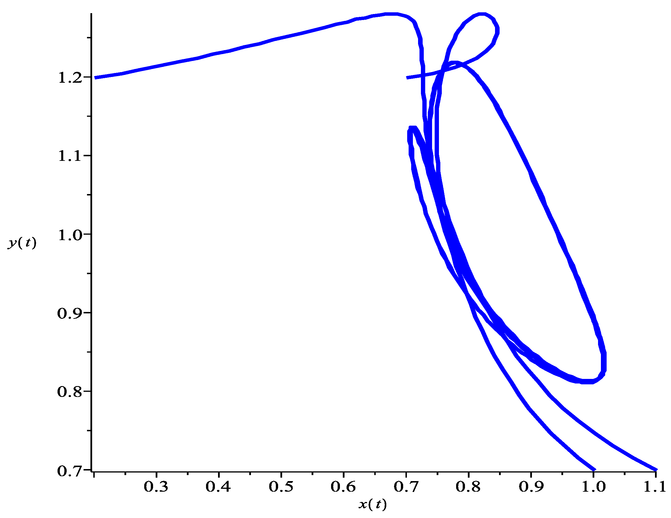
5. Numeric Simulations

Now let us consider the following three examples.
Example 1.
Consider the following system.
d x d t = x a 1 x + c 1 y 1 + x + y + x y , d y d t = y ( 1 y ) .
In this system, corresponding to system (3), we take b 1 = d 1 = e 1 = f 1 = g 1 = a 2 = b 2 = 1 .
(1) 
Now take a 1 = 2 , c 1 = 1 , then c 1 = 1 < 4 = a 1 f 1 + a 1 d 1 b 2 a 2 ; it follows from Theorem 3 that ( 0 , 1 ) is globally stable. Numeric simulation (Figure 1) supports this assertion.
(2) 
Now take a 1 = 1 2 , c 1 = 2 ; then, c 1 = 2 > 1 = a 1 f 1 + a 1 d 1 b 2 a 2 , and it follow from Theorem 4 that the unique positive equilibrium ( 0.28 , 1 ) is globally stable. Numeric simulation (Figure 2) supports this assertion.
Example 2.
Consider the following system.
d x d t = x ( 3 + sin ( t ) ) x + ( 0.75 + 0.25 cos ( t ) ) y 1 + x + y + x y , d y d t = y ( 1 y ) .
In this system, corresponding to system (3), we take b 1 = d 1 = e 1 = f 1 = g 1 = a 2 = b 2 = 1 . a 1 = 3 + sin ( t ) , c 1 = 0.75 + 0.25 cos ( t ) . By simple computation, we have a 1 L = 2 , c 1 M = 1 , M 2 = m 2 = 1 . One could easily verify the following.
a 1 L = 2 > 1 2 = c 1 M M 2 d 1 L + f 1 L m 2 .
Hence, it follows from Theorem 5 that the first species will be driven to extinction. Figure 3 supports this assertion.
Example 3.
Consider the following system.
d x d t = x ( 1 + sin ( t ) 2 ) x + ( 7 + cos ( t ) 4 ) y 1 + x + y + x y , d y d t = y 1 + 0.2 sin ( t ) ( 1 0.2 cos ( t ) ) y .
In this system, corresponding to system (3), we take b 1 = d 1 = e 1 = f 1 = g 1 = a 2 = b 2 = 1 . a 1 = 1 + sin ( t ) 2 , c 1 = 7 + cos ( t ) 4 , a 2 = 1 + 0.2 sin ( t ) , and b 2 = 1 0.2 cos ( t ) . By simple computation, we have a 1 M = 3 2 , c 1 L = 27 4 , m 2 = 2 3 , M 2 = 3 2 , d 1 M = f 1 M = 1 . One could easily verify that the following is the case.
a 1 M = 3 2 < 9 5 = c 1 L m 2 d 1 M + f 1 M M 2 .
Hence, it follows from Theorem 6 that the system is permanent. Figure 4 supports this assertion.

6. Conclusions

Stimulated by recent work of Wu and Li [37], we proposed a two-species obligate commensal symbiosis model with Crowley–Martin functional responses. Such forms of functional response take many famous functional responses as its special case: Holling II functional response, ratio-dependent functional response, and Bedditon-0DeAngelis functional response, etc.
For autonomous case, we showed that the conditions that ensure the existence of the positive equilibrium is coincident to the conditions of the global stability of positive equilibrium, which means that if the positive equilibrium exists, it is a globally stable one; consequently, two species could be coexistent in the long run. In this case, the system has no positive equilibrium, and we showed that the first species involves extinction, while the second species is globally stable. Our results showed that, for the obligate system, the commensal effect may be one of the most important factors to avoid the extinction of the species.
For the nonautonomous case, by using the differential inequality theory, we also could establish sufficient conditions to ensure the persistence or extinction of the system.
We mention here that, in our main results Theorems 3 and 4, coefficients e 1 and g 1 have no influence on the persistent property of the system; that is, the mutual interferences of the first species have no influence on the persistence or extinction property of the system. The strength of the commensalism plays an essential role on the persistence property of the system.
One of the anonymous reviewers thought it is better for us to add a numerical example to show the persistence property of the system; we add Example 3, from numerical simulation (Figure 4) and we found that, indeed, the system admits a unique T periodic solution, which is globally attractive; however, we could not prove this assertion at present, and we leave this for future investigation.

Author Contributions

All authors contributed equally to the writing of this paper. All authors have read and agreed to the published version of the manuscript.

Funding

The research was supported by Educational and scientific research projects for young and middle-aged teachers of Fujian Province (Science and Technology) (JAT200690) and the Natural Science Foundation of Fujian Province (2019J01841 and 2021J011155).

Institutional Review Board Statement

Not applicable.

Informed Consent Statement

Not applicable.

Data Availability Statement

Not applicable.

Acknowledgments

The authors would like to thank three anonymous reviewers for their valuable comments, which greatly improved the final expression of the paper.

Conflicts of Interest

The authors declare no conflict of interest.

References

  1. Su, Q.; Chen, F. The influence of partial closure for the populations to a non-selective harvesting Lotka-Volterra discrete amensalism model. Adv. Differ. Equations 2019, 2019, 281. [Google Scholar] [CrossRef]
  2. Zhu, Z.; Chen, F.; Lai, L.; Li, Z. Dynamic behaviors of a discrete May type cooperative system incorporating Michaelis-Menten type harvesting. IAENG Int. J. Appl. Math. 2020, 50, 1–10. [Google Scholar]
  3. Zhu, Z.; Wu, R.; Chen, F.; Li, Z. Dynamic behaviors of a Lotka-Volterra commensal symbiosis model with non-selective Michaelis-Menten type harvesting. IAENG Int. J. Appl. Math. 2020, 50, 396–404. [Google Scholar]
  4. Georgescu, P.; Maxin, D.; Zhang, H. Global stability results for models of commensalism. Int. J. Biomath. 2017, 10, 1750037. [Google Scholar] [CrossRef]
  5. Deng, M. Stability of a stochastic delay commensalism model with Lévy jumps. Phys. A Stat. Mech. Its Appl. 2019, 527, 121061. [Google Scholar] [CrossRef]
  6. Gakkhar, S.; Gupta, K. A three species dynamical system involving prey-predation, competition and commensalism. Appl. Math. Comput. 2016, 273, 54–67. [Google Scholar] [CrossRef]
  7. Mougi, A. The roles of amensalistic and commensalistic interactions in large ecological network stability. Sci. Rep. 2016, 6, 29929. [Google Scholar] [CrossRef] [Green Version]
  8. Han, R.; Chen, F.; Xie, X.; Miao, Z. Global stability of May cooperative system with feedback controls. Adv. Differ. Equ. 2015, 2015, 360. [Google Scholar] [CrossRef] [Green Version]
  9. Wei, Z.; Xia, Y.; Zhang, T. Stability and bifurcation analysis of a commensal model with additive Allee effect and nonlinear growth rate. Int. J. Bifurc. Chaos 2021, 31, 2150204. [Google Scholar] [CrossRef]
  10. Wu, R.; Li, L.; Zhou, X. A commensal symbiosis model with Holling type functional response. J. Math. Comput. Sci. 2016, 16, 364–371. [Google Scholar] [CrossRef] [Green Version]
  11. Xie, X.; Miao, Z.; Xue, Y. Positive periodic solution of a discrete Lotka-Volterra commensal symbiosis model. Commun. Math. Biol. Neurosci. 2015, 2015, 10. [Google Scholar]
  12. Chen, B. The influence of commensalism on a Lotka-Volterra commensal symbiosis model with Michaelis-Menten type harvesting. Adv. Differ. Equ. 2019, 2019, 43. [Google Scholar] [CrossRef] [Green Version]
  13. Liu, Y.; Xie, X.; Lin, Q. Permanence, partial survival, extinction, and global attractivity of a nonautonomous harvesting Lotka-Volterra commensalism model incorporating partial closure for the populations. Adv. Differ. Equ. 2018, 2018, 211. [Google Scholar] [CrossRef] [Green Version]
  14. Deng, H.; Huang, X. The influence of partial closure for the populations to a harvesting Lotka-Volterra commensalism model. Commun. Math. Biol. Neurosci. 2018, 2018, 10. [Google Scholar]
  15. Xue, Y.; Xie, X.; Lin, Q. Almost periodic solutions of a commensalism system with Michaelis-Menten type harvesting on time scales. Open Math. 2019, 17, 1503–1514. [Google Scholar] [CrossRef]
  16. Lei, C. Dynamic behaviors of a stage-structured commensalism system. Adv. Differ. Equ. 2018, 2018, 301. [Google Scholar] [CrossRef] [Green Version]
  17. Lin, Q. Allee effect increasing the final density of the species subject to the Allee effect in a Lotka-Volterra commensal symbiosis model. Adv. Differ. Equ. 2018, 2018, 196. [Google Scholar] [CrossRef]
  18. Chen, B. Dynamic behaviors of a commensal symbiosis model involving Allee effect and one party can not survive independently. Adv. Differ. Equ. 2018, 2018, 212. [Google Scholar] [CrossRef]
  19. Wu, R.; Li, L.; Lin, Q. A Holling type commensal symbiosis model involving Allee effect. Commun. Math. Biol. Neurosci. 2018, 2018, 6. [Google Scholar]
  20. Lei, C. Dynamic behaviors of a Holling type commensal symbiosis model with the first species subject to Allee effect. Commun. Math. Biol. Neurosci. 2019, 2019, 3. [Google Scholar]
  21. Vargas-De-León, C.; Gómez-Alcaraz, G. Global stability in some ecological models of commensalism between two species. Biomatemática 2013, 23, 139–146. [Google Scholar]
  22. Chen, F.; Xue, Y.; Lin, Q.; Xie, X. Dynamic behaviors of a Lotka-Volterra commensal symbiosis model with density dependent birth rate. Adv. Differ. Equ. 2018, 2018, 296. [Google Scholar] [CrossRef]
  23. Han, R.; Chen, F. Global stability of a commensal symbiosis model with feedback controls. Commun. Math. Biol. Neurosci. 2015, 2015, 15. [Google Scholar]
  24. Guan, X.; Chen, F. Dynamical analysis of a two species amensalism model with Beddington-DeAngelis functional response and Allee effect on the second species. Nonlinear Anal. Real World Appl. 2019, 48, 71–93. [Google Scholar] [CrossRef]
  25. Li, T.; Lin, Q.; Chen, J. Positive periodic solution of a discrete commensal symbiosis model with Holling II functional response. Commun. Math. Biol. Neurosci. 2016, 2016, 22. [Google Scholar]
  26. Puspitasari, N.; Kusumawinahyu, W.M.; Trisilowati, T. Dynamic analysis of the symbiotic model of commensalism and parasitism with harvesting in commensal populations. JTAM (J. Teor. Apl. Mat.) 2021, 5, 193–204. [Google Scholar] [CrossRef]
  27. Jawad, S. Study the dynamics of commensalism interaction with Michaels-Menten type prey harvesting. Al-Nahrain J. Sci. 2022, 25, 45–50. [Google Scholar] [CrossRef]
  28. Kumar, G.B.; Srinivas, M.N. Influence of spatiotemporal and noise on dynamics of a two species commensalism model with optimal harvesting. Res. J. Pharm. Technol. 2016, 9, 1717–1726. [Google Scholar] [CrossRef]
  29. Li, T.; Wang, Q. Stability and Hopf bifurcation analysis for a two-species commensalism system with delay. Qual. Theory Dyn. Syst. 2021, 20, 83. [Google Scholar] [CrossRef]
  30. Puspitasari, N.; Kusumawinahyu, W.M.; Trisilowati, T. Dynamical analysis of the symbiotic model of commensalism in four populations with Michaelis-Menten type harvesting in the first commensal population. JTAM (J. Teor. Apl. Mat.) 2021, 5, 392–404. [Google Scholar]
  31. Zhou, Y.C.; Jin, Z.; Qin, J.L. Ordinary Differential Equaiton and Its Application; Science Press: Beijing, China, 2003. [Google Scholar]
  32. Zhu, Z.; Chen, Y.; Li, Z.; Chen, F. Stability and bifurcation in a Leslie-Gower predator-prey model with Allee effect. Int. J. Bifurc. Chaos 2022, 32, 2250040. [Google Scholar] [CrossRef]
  33. Chen, L.; Liu, T.; Chen, F. Stability and bifurcation in a two-patch model with additive Allee effect. AIMS Math. 2022, 7, 536–551. [Google Scholar] [CrossRef]
  34. Yang, L.Y.; Han, R.Y.; Xue, Y.L.; Chen, F.D. On a nonautonomous obligate Lotka-Volterra model. J. Sanming Univ. 2014, 31, 15–18. [Google Scholar]
  35. Chen, F.D.; Lin, C.T.; Yang, L.Y. On a discrete obligate Lotka-Volterra model with one party can not surivive independently. J. Shenyang Univ. (Natural Sci.) 2015, 27, 336–338. [Google Scholar]
  36. Chen, F.; Pu, L.; Yang, L. Positive periodic solution of a discrete obligate Lotka-Volterra model. Commun. Math. Biol. Neurosci. 2015, 2015, 14. [Google Scholar]
  37. Wu, R.; Li, L. Dynamic behaviors of a commensal symbiosis model with ratio-dependent functional response and one party can not survive independently. J. Math. Comput. Sci. 2016, 16, 495–506. [Google Scholar] [CrossRef] [Green Version]
  38. Holling, C.S. The functional response of predators to prey density and its role in mimicry and population regulation. Mem. Entomol. Soc. Can. 1965, 97, 5–60. [Google Scholar] [CrossRef] [Green Version]
  39. Yu, S.; Chen, F. Almost periodic solution of a modified Leslie-CGower predator-Cprey model with Holling-type II schemes and mutual interference. Int. J. Biomath. 2014, 7, 1450028. [Google Scholar] [CrossRef]
  40. Molla, H.; Sarwardi, S.; Sajid, M. Predator-prey dynamics with Allee effect on predator species subject to intra-specific competition and nonlinear prey refuge. J. Math. Comput. Sci. 2022, 25, 150–165. [Google Scholar] [CrossRef]
  41. Roy, J.; Barman, D.; Alam, S. Role of fear in a predator-prey system with ratio-dependent functional response in deterministic and stochastic environment. Biosystems 2020, 197, 104176. [Google Scholar] [CrossRef]
  42. Pal, S.; Majhi, S.; Mandal, S.; Pal, N. Role of fear in a predator-prey model with Beddington-DeAngelis functional response. Z. Naturforschung A 2019, 74, 581–595. [Google Scholar] [CrossRef]
  43. Crowley, P.H.; Martin, E.K. Functional responses and interference within and between year classes of a dragonfly population. J. N. Am. Benthol. Soc. 1989, 8, 211–221. [Google Scholar] [CrossRef]
  44. Tripathi, J.P.; Bugalia, S.; Tiwari, V.; Kang, Y. A predator-prey model with Crowley-Martin functional response: A nonautonomous study. Nat. Resour. Model. 2020, 33, E12287. [Google Scholar] [CrossRef]
Figure 1. Stability of boundary equilibrium (0,1); here, we take a 1 = 2 , c 1 = 1 , which includes initial conditions ( x ( 0 ) , y ( 0 ) ) = ( 1 , 0.3 ) , ( 0.4 , 2 ) , ( 1 , 0.02 ) , ( 1 , 2 ) , and ( 1 , 1.2 ) .
Axioms 11 00298 g001
Figure 2. Stability of positive equilibrium (0.28,1); here we take a 1 = 1 2 , c 1 = 2 , which includes the initial conditions ( x ( 0 ) , y ( 0 ) ) = ( 0.04 , 2 ) , ( 0.5 , 0.2 ) , ( 0.5 , 0.02 ) , ( 0.5 , 0.4 ) , ( 0.2 , 2 ) , and ( 0.01 , 2 ) .
Axioms 11 00298 g002
Figure 3. Extinction of the first species; here, we take a 1 = 3 + sin ( t ) , c 1 = 0.75 + 0.25 cos ( t ) , which includes the initial conditions ( x ( 0 ) , y ( 0 ) ) = ( 0.5 , 2 ) , ( 0.4 , 0.02 ) , ( 0.1 , 0.4 ) , and ( 0.2 , 2 ) .
Axioms 11 00298 g003
Figure 4. Attractively of solutions; here, we take a 1 = 1 + sin ( t ) 2 , c 1 = 7 + cos ( t ) 4 , a 2 = 1 + 0.2 sin ( t ) , ajnd b 2 = 1 0.2 cos ( t ) . The initial conditions are ( x ( 0 ) , y ( 0 ) ) = ( 1.0 , 0.7 ) , ( 1.1 , 0.7 ) , ( 0.7 , 1.2 ) , and ( 0.2 , 1.2 ) .
Axioms 11 00298 g004
Publisher’s Note: MDPI stays neutral with regard to jurisdictional claims in published maps and institutional affiliations.

