Article

On the Bias in Confirmatory Factor Analysis When Treating Discrete Variables as Ordinal Instead of Continuous

by
Alexander Robitzsch
1,2
1
IPN—Leibniz Institute for Science and Mathematics Education, 24118 Kiel, Germany
2
Centre for International Student Assessment (ZIB), 24118 Kiel, Germany
Axioms 2022, 11(4), 162; https://doi.org/10.3390/axioms11040162
Submission received: 5 March 2022 / Revised: 29 March 2022 / Accepted: 30 March 2022 / Published: 1 April 2022
(This article belongs to the Collection Mathematical Analysis and Applications)

Abstract

:
Confirmatory factor analysis is some of the most widely used statistical techniques in the social sciences. Frequently, variables (i.e., items) stemming from questionnaires are analyzed. Two competing approaches for estimating confirmatory factor analysis can be distinguished. First, ordinal variables could be treated as in the case of continuous variables using Pearson correlations, and maximum likelihood estimation method would be applied. Second, an ordinal factor analysis based on polychoric correlations can be fitted. In the majority of the psychometric literature, there is a preference for the ordinal factor analysis based on polychoric correlations because the continuous treatment of variables results in biased factor loadings and biased factor correlations. This article argues that it is not legitimate to speak about bias when comparing the two competing factor analytic approaches because it depends on how true model parameters are defined. This decision can be made individually by a researcher. It is shown in simulation studies and analytical derivations that treating variables ordinally using polychoric correlations instead of continuous using Pearson correlations can also lead to biased estimates of factor loadings and factor correlations. Consequently, it should only be stated that different model parameters are defined in a continuous and an ordinal treatment, and one approach should not generally be preferred over the other.

1. Introduction

Confirmatory factor analysis is frequently applied in social science research. Frequently, variables (i.e., items) stemming from questionnaires are analyzed. The variables are often discrete and have a finite number of ordered categories. Applied researchers are often searching for an adequate approach for factor analysis for ordinal variables. Two competing approaches can be distinguished. First, ordinal variables could be treated as in the case of continuous variables using Pearson correlations, and the same maximum likelihood estimation method would be applied. Second, an ordinal factor analysis based on polychoric correlations can be fitted that is claimed to take the ordinal nature of the variables into account. In the majority of the psychometric literature, there is a preference for the ordinal factor analysis based on polychoric correlations [1,2,3,4,5,6,7]. The main message of these articles is that ordinal variables should be treated as ordinal (i.e., not being treated as continuous variables) if there are only a few categories per item or the marginal distributions are skewed (e.g., [6]). In a previous article, we argued that treating ordinal variables as continuous can always be defended. The argument for doing so does neither depend on the number of categories nor the marginal distribution of ordinal variables [8]. Moreover, we argued that no simulation studies would be required to demonstrate this reasoning [8]. However, we feel that it is valuable to provide further evidence for our reasoning by presenting simulation studies and analytical results. We conclude that it is not legitimate to speak about bias when comparing the two competing factor analytic approaches.
The rest of the article is structured as follows. In Section 2, we discuss the two competing approaches for the factor analysis model. Section 3 presents results from two simulation studies. In Section 4, we discuss analytical findings. Finally, the paper closes with a discussion in Section 5.

2. Factor Analysis for Ordinal Items

2.1. Gaussian Copula Model for Ordinal Items

In the following, we present a multivariate distribution for discrete data. This distribution is referred to as the Gaussian copula [9,10,11]. In psychometrics, it is also known as the underlying latent variable approach [12].
Assume that there is a vector of variables (i.e., items) Y = ( Y 1 , , Y I ) . Each of the variables has integer categories 1 , , K i . Now, assume that there are underlying standard normally distributed latent variables Y i * for the integer-valued variable Y i for i = 1 , , I . Denote by Y * the vector containing the underlying latent variables. and Y i * is discretized by means of a vector of thresholds = τ Y i , 0 < τ Y i , 1 < < τ Y i , K i < τ Y i , K i + 1 = . Then, the discrete variable Y i takes the value h if Y i * lies within the interval [ τ Y i , h 1 , τ Y i , h ) . The multivariate vector Y * follows a multivariate normal distribution with a correlation matrix Σ * . Recall that all variables in Y * have zero means and variances of one. By prescribing thresholds τ for all variables, the discrete probability distribution is given as
P ( Y i = h , Y j = l ) = Φ 2 ( τ Y i , h , τ Y i , l ; ρ Y i Y j * ) Φ 2 ( τ Y i , h 1 , τ Y i , l ; ρ Y i Y j * ) Φ 2 ( τ Y i , h , τ Y i , l 1 ; ρ Y i Y j * ) + Φ 2 ( τ Y i , h 1 , τ Y i , l 1 ; ρ Y i Y j * ) ,
where ρ Y i Y j * is the correlation of the underlying latent variables and Φ 2 ( x , y ; ρ ) is the cumulative distribution function of the bivariate standard normal distribution.
Means, variances, and covariances of the components of the discrete variable Y can be computed using the discrete distribution in Equation (1) (see [13]). Hence, one can also determine the manifest correlation ρ Y i Y j = Cov ( Y i , Y j ) / ( SD ( Y i ) SD ( Y j ) ) (i.e., Pearson correlation) for the integer-valued variables Y i and Y j . While ρ Y i * Y j * can take values within the interval [ 1 , 1 ] , the Pearson correlation is bounded, where the bounds are determined by the marginal distribution of Y i and Y j [14,15,16].
Given an observed discrete distribution of Y , one can determine the so-called polychoric correlation ρ Y i Y j * [12,17]. It can be shown that there is a monotone relation between the polychoric correlation ρ Y i Y j * and the Pearson correlation ρ Y i Y j [18]. This property can be used to simulate discrete ordinal data [19,20]. First, the discrete marginal distributions P ( Y i = h ) are fixed. These probabilities directly translate into thresholds τ Y i , h by noting that
Φ ( τ Y i , h ) = l = 1 h P ( Y i = l ) ,
where Φ is the distribution function of the standard normal distribution. The specification in Equation (2) implies that a Gaussian marginal distribution is assumed for the underlying latent variables Y i * (i.e., latent normality; see [8]). Next, fix a correlation matrix Σ for the vector of discrete variables Y . Using (1), one solves a nonlinear equation ρ Y i Y j = f ( ρ Y i Y j * ) for every pair of variables Y i and Y j for obtaining the polychoric correlation ρ Y i Y j * [20]. As a result, a matrix Σ * involving the polychoric correlations is obtained as a function of all thresholds τ and the Pearson correlation matrix Σ .
In simulations in psychometrics, one often generates data from Y * and a prespecified polychoric correlation matrix Σ * . As a consequence, a Pearson correlation matrix Σ is obtained for the discrete data Y . A frequent reasoning is that by treating variables continuously when Pearson correlations are computed, biased estimates are obtained because the estimates are usually smaller (in absolute values) than the “true” polychoric correlations. However, this reasoning depends on how truth is defined. Indeed, one can also argue that Pearson correlations are the quantity of interest. When polychoric correlations are computed, biased estimations will emerge. These reflections demonstrate that it does not make sense to speak about bias. It is up to the choice of a researcher whether Pearson or polychoric correlations are of interest. Instead of speaking about bias, one can only argue that one statistical parameter is of less interest (i.e., less adequate in a practical application) than another.

2.2. Factor Model for Pearson Correlations and Polychoric Correlations

In factor analysis, the vector of multivariate variables is represented by a vector of factor variables of lower dimension. This means that a covariance (or a correlation) matrix is represented by a common part that is attributed to factors and a residual part that represents item uniqueness [21]. A correlation is represented as
Σ Λ Ψ Λ + Θ ,
where Λ is the matrix of factor loadings, Ψ is the correlation matrix of factor variables, and Θ is a diagonal matrix of residual variances. Frequently, a particular structure in Λ (i.e., a loading structure) is prescribed that determines which variables Y i load on which factors [21]. Such a specification is labeled as confirmatory factor analysis (CFA).
The most prominent options appearing in the literature for modeling ordinal variables in CFA are treating the variables continuously and ordinally [13]. In the first case, Pearson correlations Σ are used for modeling the factor structure. In the latter case, polychoric correlations Σ * are used for modeling the factor structure. Hence, there can be two alternative modeling strategies for the variables Y :
Σ Λ Ψ Λ + Θ and Σ * Λ * Ψ * Λ * + Θ * .
In general, factor loadings Λ and Λ * obtained from factor models for Pearson correlations and polychoric correlations differ from each other. The same is true for the factor correlation matrices Ψ and Ψ * . Hence, researchers are often unsure which of the two approaches should be chosen. In psychometrics, it is often claimed that factor loadings and factor correlations from Pearson correlations are biased for ordinal data (e.g., [6,13]). As argued in Section 2.1, we think that it is illegitimate to speak about bias because both Pearson correlations Σ and polychoric correlations Σ * are well-defined parameters for a vector of discrete variables. Hence, both representations in (3) for modeling the factor structure are well-defined, and it is not justified to speak about a bias when utilizing one of the two alternatives. Alternatively, it is equally true that factor loadings Λ * and factor correlations Ψ * obtained from polychoric correlations are biased if a researcher is interested in Λ and Ψ stemming from the factor model for Pearson correlations. In fact, one can simulate discrete multivariate data with the factor representation in (3) for Pearson correlations and show that applying the CFA for polychoric correlations provides biased estimates (see [8]).
In the rest of the article, we want to show the differences between the two competing approaches. We illustrate that biases can occur in both approaches. If a researcher defines one approach (e.g., ordinal CFA) as the true model, then parameter estimates from the other approach (e.g., CFA based on Pearson correlations for continuous data) will be biased. However, the converse also holds true. We simulate a factor model based on Pearson correlations (as outlined in Section 2.1) and demonstrate that bias for an ordinal CFA will result. In the simulations and the analytical derivations, we are not concerned with sampling errors and compare the different estimators only at the population level (see also [13]).

3. Simulation Studies

In this section, we present two simulation studies with two-dimensional CFA models. In Simulation Study 1 (Section 3.1), we consider equal factor loadings. Simulation Study 2 (Section 3.2) replicates [6,13] and considers unequal factor loadings.

3.1. Simulation Study 1

3.1.1. Method

In Simulation Study 1, we studied a two-dimensional CFA. Each of the two factors is measured by three items (i.e., variables). We employed the same distributions as in [6]. There were discrete variables with 2 to 7 categories and were symmetric (S2, …, S7), moderately asymmetric (MA2, …, MA7), and extremely asymmetric (EA2, …, EA7) distributed. The shapes of the discrete distributions are displayed in Figure 1. Table A1 in Appendix A contains the numerical values of the marginal distributions. In each of the simulated conditions, all items had the same marginal distribution.
We varied the factor correlations ψ in three levels (i.e., 0.3, 0.5, and 0.7). We also used three factor levels for factor loadings (i.e., 0.3, 0.5, 0.7). All factor loadings in the two-dimensional CFA were set equal to each other. The residual variances were determined to obtain standardized variables (i.e., variables with a variance of 1).
Two data-generating models were used. Discrete items were simulated in which the factor model involving loadings, factor correlations, and residual variances either holds for the discrete data Y (“Simulated cont”) or the underlying continuous data Y * (“Simulated cat”). If the factor model holds for Pearson correlations, the simulation approach in Section 2.2 was used. According to the factor model parameters and the marginal distributions, a Pearson correlation matrix Σ was determined in the first step. In a second step, the corresponding population polychoric correlation matrix Σ * was computed.
Moreover, three analysis models were utilized. First, one uses the population Pearson correlation matrix of the original integer-valued variable Y (method “cont”) and maximum likelihood estimation for determining model parameters. Second, the original scores were transformed to normal scores Y ˜ [22,23], where score h of item Y i received the score
z h = ϕ ( τ Y i , h 1 ) ϕ ( τ Y i , h ) Φ ( τ Y i , h ) Φ ( τ Y i , h 1 ) ,
where ϕ is the density function of the standard normal distribution. In the method “cont-adj”, a CFA model of the Pearson correlation matrix of normal scores is estimated with ML. Finally, the CFA based on polychoric correlations (method “cat”) was estimated using unweighted least squares estimation. All models were estimated using the R [24] package lavaan [25]. Note that in all simulation conditions, only population-level data is used. Hence, only asymptotic bias is investigated.

3.1.2. Results

We now show biases for factor loadings and factor correlations in the different simulation conditions. Table 1 shows the estimated factor loadings for a factor correlation of 0.5. The results for the factor correlations 0.3 and 0.7 coincide with those in Table 1. The general pattern was that biases in estimated factor loadings were more pronounced for a higher true factor loading of 0.7 than for a true loading of 0.3. If discrete items were simulated according to the CFA model for Pearson correlations (“Simulated cont”), it is evident that treating variables as categorical resulted in positively biased factor loadings. In contrast, if the CFA model was simulated for polychoric correlations (“Simulated cat”), continuous treatment of the items resulted in negatively biased factor loadings. Interestingly and similar to [22], CFA based on normal scores provided very similar estimated factor loadings to the CFA model for Pearson correlations based on the original integer scores. Similar to the findings in the literature, it can also be concluded that biases in estimated factor loadings were less pronounced for less asymmetric distributions and an increasing number of item categories.
In Table 2, estimated factor correlations are displayed as a function of true factor loading and true factor correlations. Overall, biases in factor correlations were smaller than in factor loadings. Moreover, the bias in factor correlations was more pronounced for larger true factor loadings. Biases were only of practical relevance for a few item categories (i.e., two categories) or extreme asymmetric distributions (i.e., EA). In addition, estimated factor correlations were positively biased if the CFA model holds for Pearson correlations (“Simulated cont”). At the same time, negative biases existed in a continuous treatment of items when the CFA model holds for polychoric correlations (“Simulated cat”). The latter findings replicate the simulation studies found in the literature. Unfortunately, the psychometric literature conceals the former finding.

3.1.3. Summary

As argued in Section 2.2, it is questionable speaking about bias in the comparison of a continuous or an ordinal CFA approach. Simulation Study 1 shows that can either claim that there is bias when the items are treated ordinally (i.e., using polychoric correlations) or when treated continuously (i.e., using Pearson correlations). It might be more neutral to only speak about parameter differences using different approaches.

3.2. Simulation Study 2: Unequal Loadings

Simulation Study 2 considers the case of unequal loadings in a two-dimensional CFA and is a replication of [6,13].

3.2.1. Method

In this study, we investigate a two-dimensional CFA in which each of the two factors is measured by five items. The factor loadings of the five items for each factor were 0.3, 0.4, 0.5, 0.6, and 0.7. The factor correlation was fixed to 0.3. As in Simulation Study 1, all marginal distributions of the items were equal in each simulation condition. The identical 18 marginal distributions as in Simulation Study 1 were utilized. According to the findings of Simulation Study 1, the CFA model for normal scores was not considered anymore because the results were very similar to those using Pearson correlations. Like in Simulation 1, we either assumed that the CFA model holds for Pearson correlations (“Simulated cont”) or polychoric correlations (“Simulated cat”). Then, we estimated the CFA model based on the other correlation matrix that did not correspond to the data-generating parameters. It is obvious that fitting the corresponding correlation matrix provides unbiased estimates (see also Simulation Study 1).

3.2.2. Results

Table 3 presents estimated factor loadings and factor correlations. The factor loadings are positively biased if the factor model holds for Pearson correlations, but it is fitted for polychoric correlations. Only in cases of extreme asymmetry, positive biases in factor correlations were non-negligible. In other cases, the bias in factor correlations can be considered small. In contrast, and as shown in several simulation studies such as [6], estimated factor loadings are negatively biased if the items are treated as continuous variables when the factor model holds for the polychoric correlations. Estimated factor correlations were only substantially biased for extreme asymmetric distributions and a few item categories.

3.2.3. Summary

In the original Rhemtulla et al. [6] study, it was stated that “Normal theory ML [applying CFA to Pearson correlations; added by the author] was found to be more sensitive to asymmetric category thresholds and was especially biased when estimating large factor loadings”. We demonstrated that treating discrete items ordinally by using polychoric correlations is also biased if the true CFA model holds for Pearson correlations. Statements like the one cited above are particularly dangerous in applied research because it seems to imply that there would be a univocal voice under methodologists and statisticians that either one of two approaches must always be preferred for reasons of statistical bias. We argued that these kinds of statements cannot be used to give advice on choosing an adequate estimation approach in a concrete empirical application.

4. Analytical Findings

We now provide an analytical treatment of the two-dimensional factor model for ordinal variables. The basis of our derivations is an empirically obtained relation of the polychoric correlation ρ * and the Pearson correlation ρ . We assume that the bivariate distribution of two discrete variables is represented by a Gaussian copula model (see Section 2.1). It was shown that there exists an injective relationship of ρ * and ρ . By studying the relationship for the distributions presented in Section 3.1.1, it turned out that a quadratic relationship of the square root of the correlations provided a close approximation. That is, we can empirically determine coefficients ν 1 and ν 2 such that
ρ * ν 1 ρ ( 1 ν 2 ρ ) .
Table A2 in Appendix A shows the estimated coefficients of the approximating function of the square root of the polychoric correlation ρ * as a function of the square root of the Pearson correlation ρ . The coefficient ν 1 is larger than 1 and is close to 1 for variables with many categories. Moreover, ν 1 is substantially larger than 1 for more asymmetric variables. The coefficient ν 2 is larger than 0 (except for the combination of distributions S2 and EA2; see Table A2). The coefficient ν 2 reaches 0 for variables with many categories and less asymmetrical distributions. The absolute error of the numerical approximation (4) for the range ρ [ 0 , 0.8 ] is also displayed in Table A2. It turned out that the approximation error is negligible (i.e., smaller than 0.01) for variables with at least 3 categories.
Figure 2 illustrates the relationship between the square roots of the polychoric correlation and the Pearson correlation. For two 3-category items with extreme asymmetry (i.e., EA3; see Figure 1), the functional form can be well represented as a quadratic function if the Pearson correlation is smaller than 0.8 (i.e., | ρ | < 0.8 ).

4.1. Case 1: Equal Loadings

Now, we turn to the determination of factor loadings λ and a factor correlation ψ in confirmatory factor analysis.
We assume that a two-dimensional factor model holds. Each of the two factors, X and Y, is measured by three variables. Furthermore, we assume that there are nonnegative common factor loadings λ X and λ Y for all items of a factor. Assuming three variables, the measurement model is just identified in case of unequal loadings, and there is no model misfit. For equal loadings, all pairs of correlations (i.e., polychoric and Pearson correlations) corresponding to the same factor are equal. Let λ X , λ Y , and ψ denote the parameters defined in the factor model by treating the variables continuously (i.e., using Pearson correlations) and λ X * , λ Y * , and ψ * in the factor model relying on polychoric correlations. The correlation of two items from the same scale X is given as
ρ X = λ X 2 and ρ X * = ( λ X * ) 2 ( similarly for Y ) .
For two items that measure the different factors X and Y, we get
ρ X Y = λ X λ Y ψ and ρ X Y * = λ X * λ Y * ψ * .
The Equations (5) and (6) can be used for deriving estimates for λ h and ϕ :
λ X = ρ X and λ X * = ρ X * and
ψ = ρ X Y ρ X ρ Y and ψ * = ρ X Y * ρ X * ρ Y * .
We now analyze the relations of estimated factor loadings λ X * and λ X and the estimated factor correlation ψ * and ψ . Using (7), we compute by relying on the approximation (4)
λ X * = ρ X * = ν 1 , X ρ X ( 1 ν 2 , X ρ X ) = ν 1 , X λ X ( 1 ν 2 , X λ X ) .
For values of ν 2 , X near to zero, we get from (8)
λ X * ν 1 , X λ X
The estimated factor loadings in the two competing approaches are approximately linearly related. Moreover, factor loadings obtained from polychoric correlations will be larger than those from Pearson correlations because ν 1 is typically larger than 1 (see Table A2). Thus, the finding (9) confirms the findings obtained for Simulation Study 1 (Section 3.1).
We now derive the relation for the factor correlations for the two factors. We get by again using (4)
ψ * = ρ X Y * ρ X * ρ Y * = ν 1 , X Y 2 λ X λ Y ψ 1 ν 2 , X Y λ X λ Y ψ 2 ν 1 , X 2 λ 1 2 ( 1 ν 2 , X λ X ) 2 ν 1 , Y 2 λ Y 2 ( 1 ν 2 , Y λ Y ) 2
By simplifying (10), we obtain
ψ * = ψ ν 1 * 1 ν 2 , X Y λ X λ Y ψ 2 ( 1 ν 2 , X λ X ) ( 1 ν 2 , Y λ Y ) ,
where ν 1 * = ν 1 , X Y 2 ν 1 , X ν 1 , Y . Note that ν 1 * equals 1 if all variables have the same marginal distribution. By applying the Taylor approximation ( 1 x ) 1 1 + x for the terms ( 1 ν 2 , X λ X ) and ( 1 ν 2 , Y λ Y ) , and by ignoring higher-order terms in ν 2 , we get by further simplifying (11)
ψ * ψ ν 1 * 1 + ν 2 , X λ 1 + ν 2 , Y λ 2 2 ν 2 , X Y λ 1 λ 2 ψ
For ν 2 ν 2 , X = ν 2 , Y = ν 2 , X Y and ν 1 * = ν 1 , X = ν 1 , Y = ν 1 , X Y , we obtain from (12)
ψ * ψ 1 + ν 2 λ X + λ Y λ X λ Y ψ
We now analyze the term in curly brackets in (14). First, assume λ X λ Y 0 . Then, we can write λ X = λ Y + e with e 0 . We obtain
λ X + λ Y λ X λ Y ψ = 2 λ Y + e λ Y + e λ Y ψ 2 λ Y + e λ Y + e λ Y + e = λ Y 0
Similarly, we get the same result with λ Y λ X 0 . Hence, the latent correlation based on polychoric correlations is expected to be larger than based on Pearson correlations because Equation (14) can be written as
ψ * ψ ( 1 + ν 2 C ) ,
where C and ν 2 are larger than 0. This finding also confirms the result from the simulation studies. Because the quadratic coefficient ν 2 turned out to be smaller than the deviation of linear coefficient ν 1 from 1 (see Table A2), differences between the approaches using polychoric and Pearson correlations are expected to be larger for factor loadings than for factor correlations.

4.2. Case 2: Unequal Loadings

We now turn to the case of unequal factor loadings in the two-dimensional factor model. This situation was considered in Simulation Study 2 (Section 3.2). For two items X i and X j that measure the same factor X, it holds that
ρ X i X j = λ X i λ X j and ρ X i X j * = λ X i * λ X j *
Hence, we can estimate the factor loadings λ X 1 and λ X 1 * of the first item X 1 as (see [26])
λ X 1 = ρ X 1 X 2 ρ X 1 X 3 ρ X 2 X 3
We now derive the estimate based on polychoric correlations. By using the approximation (4), we obtain
λ X 1 * = ν 1 , X 1 X 2 λ X 1 λ X 2 ( 1 ν 2 , X 1 X 2 λ X 1 λ X 2 ) ν 1 , X 1 X 3 λ X 1 λ X 3 ( 1 ν 2 , X 1 X 3 λ X 1 λ X 3 ) ν 1 , X 2 X 3 λ X 2 λ X 3 ( 1 ν 2 , X 2 X 3 λ X 2 λ X 3 ) .
By rearranging terms in (15), we get
λ X 1 * = λ X 1 ν X 1 * ( 1 ν 2 , X 1 X 2 λ X 1 λ X 2 ) ( 1 ν 2 , X 1 X 3 λ X 1 λ X 3 ) 1 ν 2 , X 2 X 3 λ X 2 λ X 3 ,
where ν X 1 * = ν 1 , X 1 X 2 ν 1 , X 1 X 3 ν 1 , X 2 X 3 . If the quadratic terms involving ν 2 can be neglected, we get from (16) the approximation
λ X 1 * λ X 1 ν X 1 *
Since ν X 1 * will typically be larger than 1, estimated factor loadings based on polychoric correlations will be larger than those obtained with Pearson correlations. This finding is also in agreement with the findings of Simulation Study 2 in Section 3.2. The factor correlation ψ is no longer be uniquely determined in the case of unequal loadings. However, one can imagine that the finding from the case of equal loadings would still be valid if reasonable assumptions would be used in a derivation. Because our analytical treatment has only illustrative character, we also do not think that a more rigorous treatment would provide more insights.

4.3. Case 3: General CFA with Simplifying Linear Assumptions

We now consider the general CFA model but make simplifying assumptions on the relationship of polychoric and Pearson correlations. In (4), we empirically demonstrated that there is a quadratic relation of ρ * and ρ . Now, we further assume that the quadratic coefficient ν 2 can be neglected. A linear relationship translates into a quadratic relationship ρ * = ν 1 2 ρ of ρ * and ρ . We also impose the additional assumption that
ν 1 , Y i Y j = κ Y i κ Y j
for variables Y i and Y j . This means that the strength of the linear relationship is determined by parameters κ Y i referring to the marginal distributions. This includes the special case that all marginal distributions in Y = ( Y 1 , , Y I ) coincide such that ν 1 = κ 2 with a common parameter κ . Now, assume that the factor model holds for Pearson correlations:
Σ = Λ Ψ Λ + Θ .
Denote by λ i the i-th row vector in Λ . Because Σ is a correlation matrix, we get the identity λ i Ψ λ i + θ i = 1 , where θ is the i-th diagonal element in Θ . Using Equation (17), we have ρ Y i * Y j * = κ Y i κ Y j ρ Y i Y j . Hence, we obtain
ρ Y i * Y j * = κ Y i κ Y j ρ Y i Y j = κ Y i κ Y j λ i Ψ λ i = λ i * Ψ * λ j * ,
where λ i * = κ Y i λ i and Ψ * = Ψ . Moreover, define the i-th diagonal element in Θ * by θ i * = θ i ( κ Y i 1 ) λ i Ψ λ i . Consequently, factor loadings are multiplied by a factor, and factor correlations remain constant. This finding resembles those in simulation studies 1 and 2 in which there is no strong deviation from the linearity assumption of ρ * and ρ . Because the parameters from the ordinal CFA model (i.e., Λ * , Ψ * , and Θ * ) can be computed from the CFA based on Pearson correlations (i.e., Λ , Ψ , and Θ ), deciding among the Pearson or the polychoric CFA model cannot be made based on model fit because either both or none of the two models will fit the data.

5. Discussion and Conclusions

This article argues that the often found recommendation for not treating ordinal variables in factor models and structural equation models as continuous is not justified. The choice for a particular modeling strategy implies that it is assumed whether the factor analysis model holds for Pearson correlations or polychoric correlations. We demonstrated that the choice could not be based on simulation studies, although some psychometric literature argues otherwise.
Our simulation studies and analytical findings illustrate that always treating items as ordinal by employing a polychoric correlation can result in biased factor loadings and factor correlations if the factor model holds for Pearson correlations. However, and in coherence with the literature, one can also show that biases were obtained when incorrectly treating ordinal variables as continuous. Hence, the discussion about potential biases relies on how the true parameters are defined. It is up to a researcher whether the factor model should be imposed on Pearson correlations or polychoric correlations. The widespread statements about the bias of model parameter when treating items as continuous instead of ordinal are therefore unjustified.
Our simulation studies and analytical derivations show that the factor loadings based on polychoric correlations are typically larger than those based on Pearson correlations. As argued in this article, loadings based on Pearson correlations are often characterized as negatively biased in the literature. The loadings are particularly small if the marginal distribution of the ordinal items is (strongly) asymmetrically distributed. However, we tend to argue that loadings based on Pearson correlations tell the researcher the right imprecision that those items provide limited information on the latent variable because the distributions of ordinal items are not well aligned with the center of the distribution of the latent factor. In item response theory, the information function can quantify such a decrease. Consequently, there are well-justified arguments for using factor loadings based on Pearson correlation and item-total correlations instead of loadings based on polychoric correlations and point-biserial correlations.
In applied research, one is frequently confronted with the argument that the normal distribution assumption is violated for ordinal items. Consequently, factor analysis must be performed based on polychoric correlations. However, it must be emphasized that the ordinal treatment presupposes that the underlying latent variables are normally distributed. It has been shown that this latent normality assumption can be tested. However, other distributional assumptions are seldom applied in research practice. In more detail, the probabilities P ( Y i k ) = G i ( λ i * F + ν i k * ) using a vector of factors F can be modeled using any monotone linking function G i . Using the probit link function G i = Φ when modeling polychoric correlations is mainly justified by computational simplicity and not model fit arguments or substantive reasons. In item response theory, the link functions G i can be more flexibly estimated using shape parameters that describe asymmetry. As we have argued elsewhere, the distributional modeling assumptions of normality (when using Pearson correlations) and latent normality (when using polychoric correlations) can be both misspecified, and there should be no general preference for one modeling strategy over the other.
Finally, in social science research, we frequently find the argument that discrete items are only “measured” at an ordinal scale level. Because variables would be attributed to an ordinal scale, only particular statistical techniques would be meaningful (i.e., defensible). We generally find such statements flawed because, in our view, the meaningfulness of a statistical operation is not a property of a variable in general but has to be separately evaluated for all statistical analyses involving this variable. Moreover, we think that the concept of ordinal scales in representational measurement theory cannot be connected to empirically testable consequences. Hence, their set of axioms is entirely unrelated to substantive theory that motivates the use of particular items and, hence, the measurement instrument as a whole. It might be wise to abandon the concept of ordinal and interval scales in social science research and from the introductory methodology course because its theory does not have foundations connected to the application of statistical techniques.

Funding

This research received no external funding.

Data Availability Statement

Not applicable.

Acknowledgments

I am very grateful to the comments of two anonymous reviewers that helped to improve this article. I particularly appreciate the overly responsive and friendly communication of the editorial office of Axioms for queries regarding the paper.

Conflicts of Interest

The author declares no conflict of interest.

Abbreviations

The following abbreviations are used in this manuscript:
CFAconfirmatory factor analysis
MLmaximum likelihood

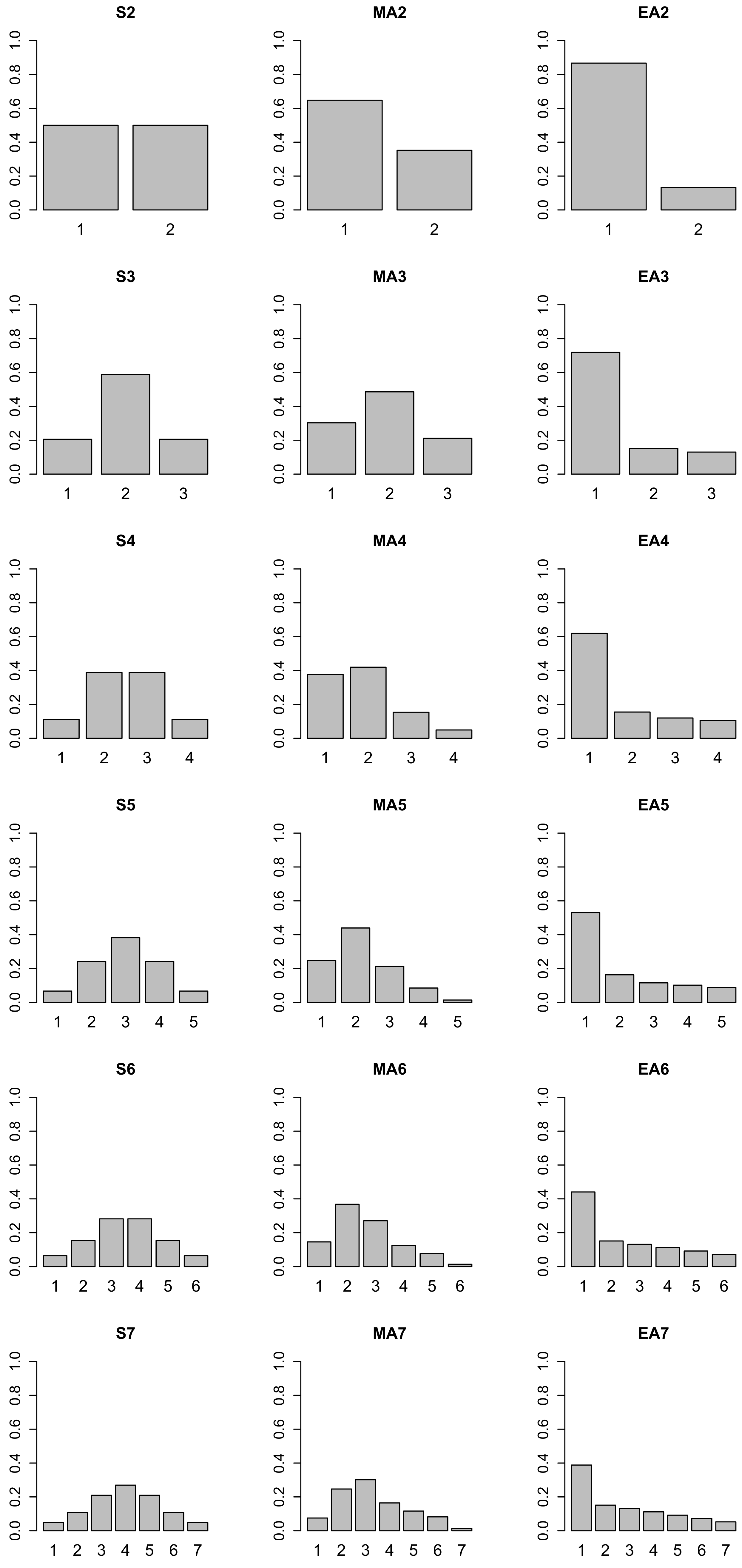
Appendix A. Data-Generating Parameters in the Simulation Studies

Table A1 contains the data-generating parameters for the marginal distributions of items. These distributions are used in Simulation Study 1 (Section 3.1), Simulation Study 2 (Section 3.2) and the empirically obtained result in Equation (4) that forms the basis of the analytical findings presented in Section 4.
Table A1. Data-generating parameters for marginal distributions of items (i.e., item-category probabilities P ( Y i = h ) for h = 1 , , K i ).
DistCat1Cat2Cat3Cat4Cat5Cat6Cat7
S20.5000.500
MA20.6480.352
EA20.8670.133
S30.2060.5890.206
MA30.3030.4860.211
EA30.7190.1510.130
S40.1120.3880.3880.112
MA40.3780.4200.1540.049
EA40.6200.1550.1200.106
S50.0670.2420.3830.2420.067
MA50.2480.4400.2130.0850.014
EA50.5310.1630.1160.1020.088
S60.0640.1540.2820.2820.1540.064
MA60.1460.3680.2710.1250.0760.014
EA60.4410.1510.1320.1120.0920.072
S70.0480.1080.2100.2690.2100.1080.048
MA70.0750.2470.3010.1640.1160.0820.014
EA70.3880.1510.1320.1120.0920.0720.053
Note. Dist = distribution type of categorical data; Cat1, …, Cat7 = category 1, …, 7; S2, …, S7 = symmetric distribution with 2 to 7 categories; MA2, …, MA7 = moderate asymmetric distribution with 2 to 7 categories; EA2, …, EA7 = extreme asymmetric distribution with 2 to 7 categories.

Appendix B. Approximation of the Relation of the Polychoric Correlation and the Pearson Correlation

Table A2 shows the estimated coefficients of the approximating function of the square root of the polychoric correlation ρ * as a function of the square root of the Pearson correlation ρ .
Table A2. Approximation ρ * ν 1 ρ ( 1 ν 2 ρ ) of the square root of the polychoric correlation ρ * as a function of the square root of the Pearson correlation ρ .
Dist1Dist2 ν 1 ν 2 Error
S2S21.3390.1610.013
MA2MA21.3800.1910.012
EA2EA21.6920.3770.006
S2MA21.3470.1440.011
S2EA21.331−0.1540.041
MA2EA21.4550.1300.020
S3S31.1370.0210.003
MA3MA31.1300.0350.003
EA3EA31.3670.2240.006
S3MA31.1300.0210.002
S3EA31.2240.0320.007
MA3EA31.2190.0490.003
S4S41.0750.0070.001
MA4MA41.1210.0540.002
EA4EA41.2580.1660.005
S4MA41.0920.0090.001
S4EA41.1410.0140.001
MA4EA41.1810.0910.002
S5S51.0490.0040.000
MA5MA51.0850.0310.001
EA5EA51.1940.1270.004
S5MA51.0630.0040.000
S5EA51.1020.0100.001
MA5EA51.1310.0600.001
S6S61.0340.0050.000
MA6MA61.0620.0250.001
EA6EA61.1400.0920.003
S6MA61.0450.0040.000
S6EA61.0740.0110.001
MA6EA61.0960.0470.001
S7S71.0260.0040.000
MA7MA71.0460.0180.001
EA7EA71.1160.0780.003
S7MA71.0340.0040.000
S7EA71.0600.0090.000
MA7EA71.0770.0380.001
Note. Dist1 = distribution type of first variable; Dist2 = distribution type of second variable; S2, …, S7 = symmetric distribution with 2 to 7 categories; MA2, …, MA7 = moderate asymmetric distribution with 2 to 7 categories; EA2, …, EA7 = extreme asymmetric distribution with 2 to 7 categories; Error = maximum function approximation error for Pearson correlations ρ smaller than 0.8. Error entries with absolute errors larger than 0.01 are printed in bold.

References

  1. Barendse, M.T.; Oort, F.J.; Timmerman, M.E. Using exploratory factor analysis to determine the dimensionality of discrete responses. Struct. Equ. Model. Multidiscip. J. 2015, 22, 87–101. [Google Scholar] [CrossRef]
  2. DiStefano, C. The impact of categorization with confirmatory factor analysis. Struct. Equ. Model. 2002, 9, 327–346. [Google Scholar] [CrossRef]
  3. Dolan, C.V. Factor analysis of variables with 2, 3, 5 and 7 response categories: A comparison of categorical variable estimators using simulated data. Br. J. Math. Stat. Psychol. 1994, 47, 309–326. [Google Scholar] [CrossRef]
  4. Li, C.H. The performance of ML, DWLS, and ULS estimation with robust corrections in structural equation models with ordinal variables. Psychol. Methods 2016, 21, 369–387. [Google Scholar] [CrossRef]
  5. Lei, P.W. Evaluating estimation methods for ordinal data in structural equation modeling. Qual. Quant. 2009, 43, 495–507. [Google Scholar] [CrossRef]
  6. Rhemtulla, M.; Brosseau-Liard, P.É.; Savalei, V. When can categorical variables be treated as continuous? A comparison of robust continuous and categorical SEM estimation methods under suboptimal conditions. Psychol. Methods 2012, 17, 354–373. [Google Scholar] [CrossRef] [Green Version]
  7. Sass, D.A.; Schmitt, T.A.; Marsh, H.W. Evaluating model fit with ordered categorical data within a measurement invariance framework: A comparison of estimators. Struct. Equ. Model. Multidiscip. J. 2014, 21, 167–180. [Google Scholar] [CrossRef]
  8. Robitzsch, A. Why ordinal variables can (almost) always be treated as continuous variables: Clarifying assumptions of robust continuous and ordinal factor analysis estimation methods. Front. Educ. 2020, 5, 589965. [Google Scholar] [CrossRef]
  9. Barbiero, A. Inducing a target association between ordinal variables by using a parametric copula family. Austrian J. Stat. 2020, 49, 9–18. [Google Scholar] [CrossRef] [Green Version]
  10. Demirtas, H. A method for multivariate ordinal data generation given marginal distributions and correlations. J. Stat. Comput. Simul. 2006, 76, 1017–1025. [Google Scholar] [CrossRef]
  11. Braeken, J.; Kuppens, P.; De Boeck, P.; Tuerlinckx, F. Contextualized personality questionnaires: A case for copulas in structural equation models for categorical data. Multivar. Behav. Res. 2013, 48, 845–870. [Google Scholar] [CrossRef] [PubMed] [Green Version]
  12. Muthén, B. A general structural equation model with dichotomous, ordered categorical, and continuous latent variable indicators. Psychometrika 1984, 49, 115–132. [Google Scholar] [CrossRef] [Green Version]
  13. Jorgensen, T.D.; Johnson, A.R. How to derive expected values of structural equation model parameters when treating discrete data as continuous. Struct. Equ. Model. Multidiscip. J. 2022. [Google Scholar] [CrossRef]
  14. Demirtas, H.; Hedeker, D. A practical way for computing approximate lower and upper correlation bounds. Am. Stat. 2011, 65, 104–109. [Google Scholar] [CrossRef]
  15. Lee, L.F. On the range of correlation coefficients of bivariate ordered discrete random variables. Econom. Theory 2001, 17, 247–256. [Google Scholar] [CrossRef] [Green Version]
  16. Olvera Astivia, O.L.; Kroc, E.; Zumbo, B.D. The role of item distributions on reliability estimation: The case of Cronbach’s coefficient alpha. Educ. Psychol. Meas. 2020, 80, 825–846. [Google Scholar] [CrossRef] [PubMed]
  17. Olsson, U. Maximum likelihood estimation of the polychoric correlation coefficient. Psychometrika 1979, 44, 443–460. [Google Scholar] [CrossRef]
  18. Van Ophem, H. A general method to estimate correlated discrete random variables. Econom. Theory 1999, 15, 228–237. [Google Scholar] [CrossRef]
  19. Barbiero, A.; Ferrari, P.A. An R package for the simulation of correlated discrete variables. Commun. Stat. Simul. Comput. 2017, 46, 5123–5140. [Google Scholar] [CrossRef]
  20. Ferrari, P.A.; Barbiero, A. Simulating ordinal data. Multivar. Behav. Res. 2012, 47, 566–589. [Google Scholar] [CrossRef] [PubMed]
  21. Mulaik, S.A. Foundations of Factor Analysis; CRC Press: Boca Raton, FL, USA, 2009. [Google Scholar] [CrossRef]
  22. Foldnes, N.; Grønneberg, S. The sensitivity of structural equation modeling with ordinal data to underlying non-normality and observed distributional forms. Psychol. Methods 2021. [Google Scholar] [CrossRef] [PubMed]
  23. Jöreskog, K.G.; Olsson, U.H.; Wallentin, F.Y. Multivariate Analysis with LISREL; Springer: Basel, Switzerland, 2016. [Google Scholar] [CrossRef]
  24. R Core Team. R: A Language and Environment for Statistical Computing; R Core Team: Vienna, Austria, 2022; Available online: https://www.R-project.org/ (accessed on 11 January 2022).
  25. Rosseel, Y. Lavaan: An R package for structural equation modeling. J. Stat. Softw. 2012, 48, 1–36. [Google Scholar] [CrossRef] [Green Version]
  26. Steyer, R. Models of classical psychometric test theory as stochastic measurement models: Representation, uniqueness, meaningfulness, identifiability, and testability. Methodika 1989, 3, 25–60. Available online: https://bit.ly/3Js7N3S (accessed on 5 March 2022).
Figure 1. Distribution types used in simulation studies 1 and 2. S2, …, S7 = symmetric distribution with 2 to 7 categories; MA2, …, MA7 = moderate asymmetric distribution with 2 to 7 categories; EA2, …, EA7 = extreme asymmetric distribution with 2 to 7 categories.
Axioms 11 00162 g001
Figure 2. Relation of the square root of the polychoric correlation (i.e., ρ * ) and the square root of the Pearson correlation (i.e., ρ ) and its linear and quadratic approximation for two items with extreme asymmetry and three categories (i.e., distribution type EA3).
Axioms 11 00162 g002
Table 1. Simulation Study 1: Estimated factor loadings for a factor correlation of 0.5 as a function of data-generating models, estimation methods, and true factor loadings.
True Loading = 0.3True Loading = 0.7
Simulated contSimulated catSimulated contSimulated cat
Estimation MethodsEstimation MethodsEstimation MethodsEstimation Methods
Distcontcont-adjcatcontcont-adjcatcontcont-adjcatcontcont-adjcat
S20.3000.3000.3750.2400.2400.3000.7000.7000.8340.5710.5710.700
S30.3000.3000.3380.2660.2660.3000.7000.7000.7850.6230.6230.700
S40.3000.3000.3210.2800.2800.3000.7000.7000.7480.6540.6540.700
S50.3000.3000.3140.2860.2870.3000.7000.7000.7320.6690.6690.700
S60.3000.3000.3100.2910.2910.3000.7000.7000.7210.6790.6790.700
S70.3000.3000.3070.2930.2930.3000.7000.7000.7160.6840.6840.700
MA20.3000.3000.3830.2340.2340.3000.7000.7000.8390.5640.5640.700
MA30.3000.3000.3340.2690.2690.3000.7000.7000.7720.6330.6330.700
MA40.3000.3010.3300.2730.2730.3000.7000.6980.7560.6460.6450.700
MA50.3000.3010.3220.2800.2810.3000.7000.6990.7430.6590.6580.700
MA60.3000.3020.3160.2850.2870.3000.7000.7010.7310.6700.6720.700
MA70.3000.3030.3120.2890.2910.3000.7000.7030.7230.6770.6810.700
EA20.3000.3000.4470.1950.1950.3000.7000.7000.8730.5110.5110.700
EA30.3000.3010.3790.2360.2370.3000.7000.6970.8080.5870.5850.700
EA40.3000.3020.3560.2520.2540.3000.7000.6990.7800.6170.6180.700
EA50.3000.3040.3420.2620.2660.3000.7000.7010.7620.6360.6380.700
EA60.3000.3040.3310.2720.2750.3000.7000.7020.7470.6520.6540.700
EA70.3000.3040.3250.2760.2800.3000.7000.7020.7390.6600.6630.700
Note. Dist = distribution type of categorical data; S2, …, S7 = symmetric distribution with 2 to 7 categories; MA2, …, MA7 = moderate asymmetric distribution with 2 to 7 categories; EA2, …, EA7 = extreme asymmetric distribution with 2 to 7 categories; cont = ML estimation using Pearson correlations of integer scores; cont-adj = ML estimation using Pearson correlations of normal scores; cat = DWLS estimation based on polychoric correlations; Entries with absolute biases larger than 0.025 are printed in bold.
Table 2. Simulation Study 1: Estimated factor correlations as a function of data-generating models, estimation methods, true factor loadings, and true factor correlations.
True Factor Correlation = 0.3True Factor Correlation = 0.7
Simulated contSimulated catSimulated contSimulated cat
Estimation MethodsEstimation MethodsEstimation MethodsEstimation Methods
Distcontcont-adjcatcontcont-adjcatcontcont-adjcatcontcont-adjcat
True loading = 0.3
S20.3000.3000.3010.3000.3000.3000.7000.7000.7010.7000.7000.700
S30.3000.3000.3000.3000.3000.3000.7000.7000.7000.7000.7000.700
S40.3000.3000.3000.3000.3000.3000.7000.7000.7000.7000.7000.700
S50.3000.3000.3000.3000.3000.3000.7000.7000.7000.7000.7000.700
S60.3000.3000.3000.3000.3000.3000.7000.7000.7000.7000.7000.700
S70.3000.3000.3000.3000.3000.3000.7000.7000.7000.7000.7000.700
MA20.3000.3000.3030.2980.2980.3000.7000.7000.7030.6980.6980.700
MA30.3000.3000.3000.3000.3000.3000.7000.7000.7000.7000.7000.700
MA40.3000.3010.3020.2990.2990.3000.7000.7010.7020.6990.6990.700
MA50.3000.3010.3010.2990.3000.3000.7000.7010.7010.6990.7000.700
MA60.3000.3010.3010.2990.3000.3000.7000.7010.7010.6990.7000.700
MA70.3000.3000.3000.3000.3000.3000.7000.7000.7000.7000.7000.700
EA20.3000.3000.3250.2890.2890.3000.7000.7000.7230.6890.6890.700
EA30.3000.3010.3090.2940.2950.3000.7000.7010.7090.6940.6950.700
EA40.3000.3010.3060.2960.2970.3000.7000.7010.7060.6960.6970.700
EA50.3000.3010.3040.2970.2980.3000.7000.7010.7040.6970.6980.700
EA60.3000.3010.3020.2980.2990.3000.7000.7010.7020.6980.6990.700
EA70.3000.3010.3020.2980.2990.3000.7000.7010.7020.6980.6990.700
True loading = 0.7
S20.3000.3000.3290.2880.2880.3000.7000.7000.7370.6840.6840.700
S30.3000.3000.3020.2990.2990.3000.7000.7000.7040.6980.6980.700
S40.3000.3000.3010.2990.2990.3000.7000.7000.7010.6990.6990.700
S50.3000.3000.3010.2990.3000.3000.7000.7000.7010.6990.7000.700
S60.3000.3000.3010.2990.3000.3000.7000.7000.7010.6990.6990.700
S70.3000.3000.3010.3000.3000.3000.7000.7000.7010.6990.7000.700
MA20.3000.3000.3370.2830.2830.3000.7000.7000.7440.6790.6790.700
MA30.3000.3000.3060.2960.2960.3000.7000.7000.7070.6950.6950.700
MA40.3000.3030.3100.2920.2940.3000.7000.7020.7100.6910.6940.700
MA50.3000.3030.3060.2950.2980.3000.7000.7030.7060.6950.6970.700
MA60.3000.3030.3050.2960.2990.3000.7000.7030.7050.6960.6990.700
MA70.3000.3030.3030.2970.3000.3000.7000.7030.7030.6970.6990.700
EA20.3000.3000.4030.2460.2460.3000.7000.7000.7880.6420.6420.700
EA30.3000.3040.3500.2680.2710.3000.7000.7030.7480.6650.6680.700
EA40.3000.3050.3340.2750.2790.3000.7000.7040.7340.6730.6770.700
EA50.3000.3060.3250.2810.2850.3000.7000.7050.7260.6790.6840.700
EA60.3000.3050.3170.2860.2900.3000.7000.7050.7180.6840.6890.700
EA70.3000.3050.3140.2880.2920.3000.7000.7050.7150.6860.6910.700
Note. Dist = distribution type of categorical data; S2, …, S7 = symmetric distribution with 2 to 7 categories; MA2, …, MA7 = moderate asymmetric distribution with 2 to 7 categories; EA2, …, EA7 = extreme asymmetric distribution with 2 to 7 categories; cont = ML estimation using Pearson correlations of integer scores; cont-adj = ML estimation using Pearson correlations of normal scores; cat = DWLS estimation based on polychoric correlations; Entries with absolute biases larger than 0.025 are printed in bold.
Table 3. Simulation Study 2: Estimated factor loadings λ 1 , , λ 5 and factor correlations ψ as a function of data-generating models and estimation methods.
Simulated cont, Estimated catSimulated cat, Estimated cont
Parm
True
λ 1
0.3
λ 2
0.4
λ 3
0.5
λ 4
0.6
λ 5
0.7
ψ
0.3
λ 1
0.3
λ 2
0.4
λ 3
0.5
λ 4
0.6
λ 5
0.7
ψ
0.3
Dist
S20.3790.5010.6180.7300.8460.3130.2380.3190.4010.4850.5680.294
S30.3380.4510.5630.6740.7860.3010.2660.3550.4440.5330.6220.299
S40.3220.4290.5350.6420.7490.3010.2800.3730.4670.5610.6540.300
S50.3140.4190.5240.6280.7330.3000.2860.3820.4770.5730.6690.300
S60.3100.4130.5160.6190.7220.3000.2910.3880.4850.5820.6790.300
S70.3070.4100.5120.6140.7170.3000.2930.3900.4880.5860.6840.300
MA20.3880.5100.6260.7380.8530.3180.2320.3120.3940.4780.5600.290
MA30.3350.4450.5550.6640.7740.3030.2690.3590.4500.5410.6450.298
MA40.3310.4390.5460.6520.7580.3060.2720.3640.4570.5510.6580.294
MA50.3220.4290.5340.6390.7440.3040.2790.3730.4680.5630.6690.297
MA60.3160.4210.5250.6280.7320.3030.2840.3800.4760.5730.6770.297
MA70.3120.4150.5180.6210.7240.3020.2880.3850.4820.5800.5040.298
EA20.4540.5750.6860.7890.8930.3670.1910.2630.3410.4230.5820.262
EA30.3830.4980.6080.7120.8190.3310.2320.3160.4030.4930.6130.278
EA40.3590.4700.5780.6820.7870.3210.2490.3370.4280.5210.6330.283
EA50.3440.4540.5600.6630.7680.3150.2600.3510.4440.5390.6490.287
EA60.3320.4400.5450.6480.7520.3100.2700.3630.4570.5540.6580.291
EA70.3270.4330.5370.6400.7430.3090.2750.3690.4640.5610.6320.292
Note. Parm = parameter; True = true parameter value; Dist = distribution type of categorical data; S2, …, S7 = symmetric distribution with 2 to 7 categories; MA2, …, MA7 = moderate asymmetric distribution with 2 to 7 categories; EA2, …, EA7 = extreme asymmetric distribution with 2 to 7 categories; cont = ML estimation using Pearson correlations of integer scores; cont-adj = ML estimation using Pearson correlations of normal scores; cat = DWLS estimation based on polychoric correlations; Entries with absolute biases larger than 0.025 are printed in bold.
Publisher’s Note: MDPI stays neutral with regard to jurisdictional claims in published maps and institutional affiliations.

