Modified Inequalities on Center-Radius Order Interval-Valued Functions Pertaining to Riemann–Liouville Fractional Integrals

Abstract

In this paper, we shall discuss a newly introduced concept of center-radius total-ordered relations between two intervals. Here, we address the Hermite–Hadamard-, Fejér- and Pachpatte-type inequalities by considering interval-valued Riemann–Liouville fractional integrals. Interval-valued fractional inequalities for a new class of preinvexity, i.e., $\mathrm{cr}$-h-preinvexity, are estimated. The fractional operator is used for the first time to prove such inequalities involving center–radius-ordered functions. Some numerical examples are also provided to validate the presented inequalities.

1. Introduction

It is well known that if the function $\mathcal{K}:\mathbb{I}\to \mathbb{R}$ is preinvex with respect to $\psi$, i.e.,

$$\mathcal{K}\left(\mathit{g}+\ell \psi \left(\mathit{s},\mathit{g}\right)\right)\le \ell \mathcal{K}\left(\mathit{s}\right)+(1-\ell )\mathcal{K}\left(\mathit{g}\right),$$

and $\mathbb{I}\ne \varnothing \in \mathbb{R}$ is an invex set with respect to $\psi :\mathbb{I}\times \mathbb{I}\ne \varnothing \to \mathbb{R}$, then for all $\mathit{g},\mathit{s}\in \mathbb{X};\ell \in \left[0,1\right]$, we have

$$\mathcal{K}\left(\mathit{g}+\frac{1}{2}\psi (\mathit{s},\mathit{g})\right)\le \frac{1}{\psi (\mathit{s},\mathit{g})}{\int }_{\mathit{g}}^{\mathit{g}+\psi (\mathit{s},\mathit{g})}\mathcal{K}\left(\mathrm{y}\right)d\mathrm{y}\le \frac{\mathcal{K}\left(\mathit{g}\right)+\mathcal{K}\left(\mathit{s}\right)}{2}.$$

The above-mentioned inequality is a modification of the classical Hermite–Hadamard inequality given as (see [1]):

$$\mathcal{K}\left(\frac{\mathit{g}+\mathit{s}}{2}\right)\le \frac{1}{\mathit{s}-\mathit{g}}{\int }_{\mathit{g}}^{\mathit{s}}\mathcal{K}\left(\mathrm{y}\right)d\mathrm{y}{⪯}_{\mathrm{cr}}\frac{\mathcal{K}\left(\mathit{g}\right)+\mathcal{K}\left(\mathit{s}\right)}{2}.$$

The Hermite–Hadamard inequality has played an important role in the development of the theory of convex analysis. It has attracted many mathematicians and has been the source of many generalizations. One of the recent aspects of the theory of inequality has been to establish new versions of the classical Hermite–Hadamard inequality using new fractional operators.

Definition 1.

(see [2,3]) Let $\mathcal{K}\in \mathcal{L}\left[\mathit{g},\mathit{s}\right]$ on $[\mathit{g},\mathit{s}]$. Then, the left and right Riemann–Liouville fractional integrals for the order $\alpha >0$ are defined as follows:

$${\mathrm{I}}_{{\mathit{g}}^{+}}^{\alpha }\mathcal{K}\left(x\right):=\frac{1}{\Gamma \left(\alpha \right)}{\int }_{\mathit{g}}^x{\left(x-\mathtt{u}\right)}^{\alpha -1}\mathcal{K}\left(\mathtt{u}\right)d\mathtt{u}(0\leqq \mathit{g}<x<\mathit{s})$$

and

$${\mathrm{I}}_{{\mathit{s}}^{-}}^{\alpha }\mathcal{K}\left(x\right):=\frac{1}{\Gamma \left(\alpha \right)}{\int }_x^{\mathit{s}}{\left(\mathtt{u}-x\right)}^{\alpha -1}\mathcal{K}\left(\mathtt{u}\right)d\mathtt{u}(0\leqq \mathit{s}<x<\mathit{s}),$$

respectively, where $\Gamma \left(\alpha \right)={\int }_0^{\infty }{\mathtt{u}}^{\alpha -1}{e}^{-\mathtt{u}}d\mathtt{u}$ is the Euler gamma function.

To make a move in this direction, Sarikaya et al. (see [2]) improved this inequality by presenting its fractional counterpart for Riemann–Liouville fractional integrals given as:

Suppose $\mathcal{K}:[\mathit{g},\mathit{s}]\to \mathbb{R}$ is a convex function with $0\le \mathit{g}\le \mathit{s}$. If $\mathcal{K}\in \mathcal{L}[\mathit{g},\mathit{s}]$, then for $\alpha >0$,

$$\mathcal{K}\left(\frac{\mathit{g}+\mathit{s}}{2}\right)\le \frac{2^{\alpha -1}\Gamma (\alpha +1)}{{(\mathit{s}-\mathit{g})}^{\alpha }}\left[{\mathtt{I}}_{{\mathit{g}}^{+}}^{\alpha }\mathcal{K}\left(\mathit{s}\right)+{\mathtt{I}}_{{\mathit{s}}^{-}}^{\alpha }\mathcal{K}\left(\mathit{g}\right)\right]\le \frac{\mathcal{K}\left(\mathit{g}\right)+\mathcal{K}\left(\mathit{s}\right)}{2}.$$

Fractional calculus is a basic concept in applied sciences and mathematics. Researchers are driven to use fractional calculus as a tool to address many practical issues. Fractional analysis and inequality theory have coevolved in the modern age. Various fractional versions of Hermite–Hadamard-, Fejer-, Ostrowski-, and Pachpatte-type inequalities have received much attention over the years. Many scholars have used the Riemann–Liouville fractional integral operators to study the Ostrowski inequality (see [4]), Simpson-type inequality (see [5]), and Hermite–Hadamard–Mercer inequalities (see [6]) in addition to the aforementioned inequality. Through fractional integral operators of the Katugampola type, the Hermite–Hadamard inequality and its Fejér counterpart were studied by Katugampola et al. (see [7]). Fernandez and Mohammed (see [8]) employed Atangana–Baleanu fractional operators to present alternative variants of the Hermite–Hadamard inequality, and Tariq et al. (see [9]) proved Simpson–Mercer type inequalities. The Hermite–Hadamard inequality was also studied using the Caputo–Fabrizio fractional integrals (see [10,11]). Recently, Butt et al. (see [12]), presented new versions of Jensen- and Jensen–Mercer-type inequalities in the fractal sense. New fractional versions of Hermite–Hadamard–Mercer- and Pachpatte–Mercer-type inclusions have been established for convex [13] and harmonically convex functions [14], respectively. Hermite–Hadamard inequalities have been further generalized for convex interval-valued [15] and LR-Bi convex fuzzy interval-valued functions [16]. Kashuri et al. [17] established Beesack–Wirtinger-type inequalities for different convexities. Several other interesting versions of the mentioned inequalities can also be found in the literature (see [18,19,20]). This analysis discloses the strong connection shared between fractional integral operators and integral inequalities.

In this paper, we are interested in incorporating the concepts of a new type of interval-valued analysis, i.e., center–radius order with fractional calculus, to present our results. To be more specific, Hermite–Hadamard-type inequalities and their refinements, such as Pachpatte-type inequalities and Fejér-type inequalities, are discussed for interval-valued preinvex functions, the product of two preinvex functions, and symmetric functions.

Throughout this paper, we use the following notation:

• ${\mathbb{R}}_I$ is the set of all closed intervals of $\mathbb{R}$;
• ${\mathbb{R}}_I^{+}$ is the set of all positive closed intervals of $\mathbb{R}$;
• ${\mathbb{R}}_I^{-}$ is the set of all negative closed intervals of $\mathbb{R}$.

$\mathrm{cr}$-Order Relation

Let $\mathrm{e}=[\underline{\mathrm{e}},\overline{\mathrm{e}}]\in {\mathbb{R}}_I$, then the center of the interval is defined as ${\mathrm{e}}_{\mathrm{c}}=\frac{\overline{\mathrm{e}}+\underline{\mathrm{e}}}{2}$ and the radius of the interval is defined as ${\mathrm{e}}_{\mathrm{r}}=\frac{\overline{\mathrm{e}}-\underline{\mathrm{e}}}{2}$. Together, they are represented as:

$$\mathrm{e}=〈{\mathrm{e}}_{\mathrm{c}},{\mathrm{e}}_{\mathrm{r}}〉=〈\frac{\overline{\mathrm{e}}+\underline{\mathrm{e}}}{2},\frac{\overline{\mathrm{e}}-\underline{\mathrm{e}}}{2}〉.$$

Definition 2.

The center–radius-order relation for $\mathrm{e}=[\underline{\mathrm{e}},\overline{\mathrm{e}}]=\langle {\mathrm{e}}_{\mathrm{c}},{\mathrm{e}}_{\mathrm{r}}\rangle$, $\mathrm{f}=[\underline{\mathrm{f}},\overline{\mathrm{f}}]=\langle {\mathrm{f}}_{\mathrm{c}},{\mathrm{f}}_{\mathrm{r}}\rangle \in {\mathbb{R}}_I$ is defined as:

$$\mathrm{e}{⪯}_{\mathrm{cr}}\mathrm{f}⟺\left\{\begin{array}{cc}{\mathrm{e}}_{\mathrm{c}}<{\mathrm{f}}_{\mathrm{c}},\hfill & \mathrm{if}{\mathrm{e}}_{\mathrm{c}}\ne {\mathrm{f}}_{\mathrm{c}};\hfill \\ {\mathrm{e}}_{\mathrm{r}}\le {\mathrm{f}}_{\mathrm{r}},\hfill & \mathrm{if}{\mathrm{e}}_{\mathrm{c}}={\mathrm{f}}_{\mathrm{c}}.\hfill \end{array}\right.$$

We have either $\mathrm{e}{⪯}_{\mathrm{cr}}\mathrm{f}$ or $\mathrm{f}{⪯}_{\mathrm{cr}}\mathrm{e}$ for any two intervals $\mathrm{e},\mathrm{f}\in {\mathbb{R}}_I$.

Definition 3.

(see [21]) Let $\mathcal{K}:[\mathit{g},\mathit{s}]\subset \mathbb{R}$ be an interval-valued function defined as

$$\mathcal{K}=[\underline{\mathcal{K}},\overline{\mathcal{K}}].$$

Then, we say the function $\mathcal{K}$ is Riemann integrable over $[\mathit{g},\mathit{s}]$, if and only if $\underline{\mathcal{K}}$ and $\overline{\mathcal{K}}$ are Riemann integrable over $[\mathit{g},\mathit{s}]$, i.e.,

$$\left(IR\right){\int }_{\mathit{g}}^{\mathit{s}}\mathcal{K}\left(\mathtt{u}\right)d\mathtt{u}=\left[\left(R\right){\int }_{\mathit{g}}^{\mathit{s}}\underline{\mathcal{K}}\left(\mathtt{u}\right)d\mathtt{u},\left(R\right){\int }_{\mathit{g}}^{\mathit{s}}\overline{\mathcal{K}}\left(\mathtt{u}\right)d\right].$$

The set of all Riemann-integrable interval-valued functions over $[\mathit{g},\mathit{s}]$ are represented by ${\mathcal{IR}}_{\left(\right[\mathit{g},\mathit{s}\left]\right)}$.

Corollary 1.

Let $\mathcal{K}:[\mathit{g},\mathit{s}]$ be an interval-valued mapping such that $\mathcal{K}=\left[\underline{\mathcal{K}},\overline{\mathcal{K}}\right]$ with $\underline{\mathcal{K}},\overline{\mathcal{K}}\in {\mathbb{R}}_{[\mathit{g},\mathit{s}]}$. Then

$${\mathrm{I}}_{{\mathit{g}}^{+}}^{\alpha }\mathcal{K}\left(x\right)=\left[{\mathrm{I}}_{{\mathit{g}}^{+}}^{\alpha }\underline{\mathcal{K}}\left(x\right),{\mathrm{I}}_{{\mathit{g}}^{+}}^{\alpha }\overline{\mathcal{K}}\left(x\right)\right]$$

and

$${\mathrm{I}}_{{\mathit{s}}^{-}}^{\alpha }\mathcal{K}\left(x\right)=\left[{\mathrm{I}}_{{\mathit{s}}^{-}}^{\alpha }\underline{\mathcal{K}}\left(x\right),{\mathrm{I}}_{{\mathit{s}}^{-}}^{\alpha }\overline{\mathcal{K}}\left(x\right)\right].$$

Shi et al. (see [22]) improved the properties of integration and explained that it preserves the order with respect to the $\mathrm{cr}$-order as well.

Theorem 1.

Let the two interval-valued functions $\mathcal{K},\mathcal{G}:[\mathit{g},\mathit{s}]\subset \mathbb{R}$ be defined as

$$\mathcal{K}=[\underline{\mathcal{K}},\overline{\mathcal{K}}]\mathit{and}\mathcal{G}=[\underline{\mathcal{G}},\overline{\mathcal{G}}].$$

Then,

$${\int }_{\mathit{g}}^{\mathit{s}}\mathcal{K}\left(\mathtt{u}\right)d\mathtt{u}{⪯}_{\mathrm{cr}}{\int }_{\mathit{g}}^{\mathit{s}}\mathcal{G}\left(\mathtt{u}\right)d\mathtt{u}$$

holds if $\mathcal{K}\left(\mathtt{u}\right){⪯}_{\mathrm{cr}}\mathcal{G}\left(\mathtt{u}\right)$ for all $\mathtt{u}\in [\mathit{g},\mathit{s}]$.

Example 1.

Let $\mathcal{K}=[\mathtt{u},\mathtt{u}+1]$ and $\mathcal{G}=[{\mathtt{u}}^2+1,2\mathtt{u}+1]$. Then for $\mathtt{u}\in [0,1]$

$${\mathcal{K}}_{\mathrm{c}}=\mathtt{u}+\frac{1}{2},{\mathcal{K}}_{\mathrm{r}}=\frac{1}{2},{\mathcal{G}}_{\mathrm{c}}=\frac{{\mathtt{u}}^2+2\mathtt{u}+2}{2}\mathit{and}{\mathcal{G}}_{\mathrm{r}}=\frac{2\mathtt{u}-{\mathtt{u}}^2}{2}.$$

From Definition 2, we have $\mathcal{K}\left(\mathtt{u}\right){⪯}_{\mathrm{cr}}\mathcal{G}\left(\mathtt{u}\right)$, $\mathtt{u}\in [0,1]$ since

$${\int }_0^1[\mathtt{u},\mathtt{u}+1]d\mathtt{u}=\left[\frac{1}{2},\frac{3}{2}\right]$$

and

$${\int }_0^1[{\mathtt{u}}^2+1,2\mathtt{u}+1]d\mathtt{u}=\left[\frac{4}{3},2\right].$$

Now, again using Definition 2, we have

$${\int }_0^1\mathcal{K}\left(\mathtt{u}\right)d\mathtt{u}{⪯}_{\mathrm{cr}}{\int }_0^1\mathcal{G}\left(\mathtt{u}\right)d\mathtt{u}.$$

Figure 1 and Figure 2 show the graphical representation of Theorem 1.

We choose the center-radius order interval-valued analysis defined by Bhunia et al. (see [23]) among the multiple interpretations and definitions of interval-valued analysis offered by various authors (see [24,25,26,27]). Despite initially appearing to be equivalent, each specified notion and its definitions are entirely distinct. Numerous researchers have connected various convex functions and integral inequalities within the framework of interval-valued analysis, yielding several noteworthy results. The Ostrowski-type inequalities were examined by Chalco-Cano (see [28]), the Minkowski-type inequalities were established by Roman-Flores (see [29]), and the Opial-type inequalities were investigated by (see [30]). The interval-valued h-convex function was proposed by Zhao et al. (see [31]), who also established a refinement of the Hermite–Hadamard inequality. Left–right interval-valued and fuzzy interval-valued functions were introduced by Zhang et al. (see [26]) and Costa et al. (see [27]) to prove Jensen’s inequalities. The interval $(h1,h2)$-convex function was first described by An et al. [32]. Zhao et al. [33] improved on this idea by creating matching $\mathrm{H}-\mathrm{H}$-type inequalities and interval-valued coordinated convex functions. This was also used to support the $\mathrm{H}-\mathrm{H}-$ and Fejer-type inequalities for n-polynomial convex interval-valued functions [34] and preinvex functions [35,36]. Recently, Lai et al. [37] expanded the idea of interval-valued preinvex functions to include interval-valued coordinated preinvex functions.

The inclusion and interval of the partial lower–upper (LU) or left–right (LR) order connections are what support these findings. Therefore, it is crucial to understand how to use a total order relation to look at the convexity and inequality of interval-valued functions. In the course of this study, we deal with the complete interval order relation, or $\mathrm{cr}$-order, as proposed by Bhunia et al. [23]. Investigating the $\mathrm{cr}$-$\mathsf{h}$-preinvexity of interval-valued functions in terms of $\mathrm{cr}$-order for fractional integrals is the main objective of this study.

Recently, the use of fractional calculus and interval-valued analysis have increased exponentially with respect to integral inequalities. To move forward in this direction, it is necessary to incorporate the concepts of $\mathrm{cr}$-order interval-valued analysis and fractional calculus to present new inequalities. There have not been many studies done considering the Hermite–Hadamard inequality for center–radius $\left(\mathrm{cr}\right)$-order interval-valued functions. To fill this gap in the literature, we aim to establish some Hermite–Hadamard-type inequalities and their refinements with the help of fractional calculus, fuzzy calculus, time-scale calculus, and quantum calculus. Particularly in this article, we shall start our study by incorporating fractional calculus and interval-valued $\mathrm{cr}$-preinvexity to present our main results. In subsequent articles, we shall focus on considering these concepts in the above-mentioned directions.

The novelty of the current study is that for the first time in the literature, we employ fractional operators to establish our inequalities concerning the center–radius-ordered relation. In terms of how integral inequalities such as the Hermite–Hadamard-, Pachpatte-, and Fejér-types can be combined with the concepts of the $\mathrm{cr}$-interval-valued function, this study provides a new avenue in the subject of inequalities. Here, it is important to emphasize the distinction between the $\mathrm{cr}$-order interval-valued analysis notion and the traditional interval-valued analysis concept. Here, we calculate the intervals using the concept of center and radius defined as ${\mathrm{e}}_{\mathrm{c}}=\frac{\overline{\mathrm{e}}+\underline{\mathrm{e}}}{2}$ and ${\mathrm{e}}_{\mathrm{r}}=\frac{\overline{\mathrm{e}}-\underline{\mathrm{e}}}{2}$, respectively, where $\overline{\mathrm{e}}$ and $\underline{\mathrm{e}}$ are endpoints of an interval $\mathrm{e}$.

The rest of the paper is organized as follows: In Section 1, we review the necessary conditions and pertinent information pertaining to the associated interval-valued analysis and integral inequalities. In Section 2, we explain the concept of preinvexity and $\mathrm{cr}$-order functions. In Section 3, we derive the Hermite–Hadamard and its relevant inequalities for the $\mathrm{cr}$-$\mathtt{h}$-preinvex functions. In Section 5, we provide a succinct conclusion and discuss several open research questions that are related to the findings of this work.

2. Preliminaries

In the year 1981, Hanson (see [38]) introduced the concept of invex functions in the context of the bifunction $\psi (·,·)$. Invex sets and preinvex functions were studied by Ben-Israel and Mond (see [39]) shortly after Hanson’s study was published. Convexity is a more narrowly defined concept than preinvexity. In 1988, Weir and Mond (see [40]) investigated the theory of preinvexity using the idea of invex sets.

Definition 4.

(see [40]) Let $\mathit{g}\in \mathbb{X}\subset {\mathbb{R}}^n$; then, $\mathbb{X}$ is said to be invex at $\mathit{g}$ with respect to $\psi :\mathbb{X}\times \mathbb{X}\to {\mathbb{R}}^n$ if for each $\mathit{s}\in \mathbb{X}$,

$$\mathit{g}+\ell \psi (\mathit{s},\mathit{g})\in \mathbb{X},\ell \in [0,1].$$

Condition C.

(see [41]) Let $\mathbb{X}\subset R^n$ be an open invex subset with respect to $\psi :\mathbb{X}\times \mathbb{X}\to \mathbb{R}$. For any $\mathit{g},\mathit{s}\in \mathbb{X}$ and $\ell \in [0,1]$,

$$\psi \left(\mathit{s},\mathit{s}+\ell \psi \left(\mathit{g},\mathit{s}\right)\right)=-\ell \psi \left(\mathit{g},\mathit{s}\right),$$

(1)

and

$$\psi \left(\mathit{g},\mathit{s}+\ell \psi \left(\mathit{g},\mathit{s}\right)\right)=\left(1-\ell \right)\psi \left(\mathit{g},\mathit{s}\right).$$

(2)

In fact, using condition C, for any $\mathit{g},\mathit{s}\in \mathbb{X}$ and ${\ell }_1,{\ell }_2\in [0,1]$, one has

$$\psi \left(\mathit{s}+{\ell }_2\psi \left(\mathit{g},\mathit{s}\right),\mathit{s}+{\ell }_1\psi \left(\mathit{g},\mathit{s}\right)\right)=\left({\ell }_2-{\ell }_1\right)\psi \left(\mathit{g},\mathit{s}\right).$$

Definition 5.

(see [42]) The function $\mathcal{K}:\mathbb{I}\to \mathbb{R}$ is said to be $\mathtt{h}$-preinvex with respect to ψ if

$$\mathcal{K}\left(\mathit{g}+\ell \psi \left(\mathit{s},\mathit{g}\right)\right)\leqq \mathtt{h}(\ell )\mathcal{K}\left(\mathit{s}\right)+\mathtt{h}(1-\ell )\mathcal{K}\left(\mathit{g}\right),(\forall \mathit{g},\mathit{s}\in \mathbb{X};\ell \in \left[0,1\right]),$$

where $\mathbb{I}\ne \varnothing \in \mathbb{R}$ is an invex set with respect to $\psi :\mathbb{I}\times \mathbb{I}\ne \varnothing \to \mathbb{R}$ and $\mathtt{h}\ne 0$.

Interval-Valued $\mathrm{cr}$-$\mathtt{h}$-Preinvex Functions and Relevant Results

Sahoo et al. (see [43]) introduced the concept of interval valued $\mathrm{cr}$-$\mathtt{h}$-Preinvex function and established some alternative forms of the Hermite–Hadamard, Fejer and Pachhpatte type inclusions. The new definitions and some of their results are given as follows:

Definition 6.

Let $\mathtt{h}:[0,1]\to {\mathbb{R}}^{+}$ be a real function and $\mathcal{K}:[\mathit{g},\mathit{g}+\psi (\mathit{s},\mathit{g}\left)\right]$ be an interval-valued mapping given by $\mathcal{K}=[\underline{\mathcal{K}},\overline{\mathcal{K}}]$. Then, we say the function $\mathcal{K}$ is interval-valued $\mathrm{cr}$-$\mathtt{h}$-preinvex with respect to ψ iff

$$\mathcal{K}\left(\mathit{g}+\ell \psi \left(\mathit{s},\mathit{g}\right)\right){⪯}_{\mathrm{cr}}\mathtt{h}(\ell )\mathcal{K}\left(\mathit{s}\right)+\mathtt{h}(1-\ell )\mathcal{K}\left(\mathit{g}\right)(\forall \mathit{g},\mathit{s}\in \mathbb{X};\ell \in \left[0,1\right]).$$

Theorem 2.

Assuming $\mathcal{K}:[\mathit{g},\mathit{g}+\psi (\mathit{s},\mathit{g}\left)\right]\to \mathbb{R}$ is an interval-valued mapping, i.e.,

$$\mathcal{K}\left(\mathtt{u}\right)=\left[\underline{\mathcal{K}}\left(\mathtt{u}\right),\overline{\mathcal{K}}\left(\mathtt{u}\right)\right]$$

for all $\mathtt{u}\in \left[\mathit{g},\mathit{s}\right]$. If $\mathcal{K}:[\mathit{g},\mathit{g}+\psi (\mathit{s},\mathit{g}\left)\right]\to \mathbb{R}$ is a $\mathrm{cr}$-$\mathtt{h}$-preinvex function. Then, for $\mathtt{h}\left(\frac{1}{2}\right)>0$,

$$\frac{1}{2\mathtt{h}\left(\frac{1}{2}\right)}\mathcal{K}\left(\mathit{g}+\frac{1}{2}\psi (\mathit{s},\mathit{g})\right){⪯}_{\mathrm{cr}}\frac{1}{\psi (\mathit{s},\mathit{g})}{\int }_{\mathit{g}}^{\mathit{g}+\psi (\mathit{s},\mathit{g})}\mathcal{K}\left(\mathtt{u}\right)d\mathtt{u}{⪯}_{\mathrm{cr}}[\mathcal{K}\left(\mathit{g}\right)+\mathcal{K}\left(\mathit{s}\right)]{\int }_0^1\mathtt{h}\left(\mathfrak{t}\right)d\mathfrak{t},$$

holds true.

Theorem 3.

Suppose that $\mathcal{K},\mathcal{G}:[\mathit{g},\mathit{g}+\xi (\mathit{s},\mathit{g}\left)\right]\to \mathbb{R}$ is an interval-valued function given by

$$\mathcal{K}\left(\mathrm{y}\right)=\left[\underline{\mathcal{K}}\left(\mathrm{y}\right),\overline{\mathcal{K}}\left(\mathrm{y}\right)\right]\mathit{and}\mathcal{G}\left(\mathrm{y}\right)=\left[\underline{\mathcal{G}}\left(\mathrm{y}\right),\overline{\mathcal{G}}\left(\mathrm{y}\right)\right]$$

for all $\mathrm{y}\in \left[\mathit{g},\mathit{s}\right]$ and $\mathcal{K},\mathcal{G}\in {\mathcal{IR}}_{\left(\right[\mathit{g},\mathit{s}\left]\right)}$. If $\mathcal{K}:[\mathit{g},\mathit{g}+\xi (\mathit{s},\mathit{g}\left)\right]\to \mathbb{R}$ is a $\mathrm{cr}-{\mathsf{h}}_{\mathsf{1}}$-preinvex function and $\mathcal{G}:[\mathit{g},\mathit{g}+\xi (\mathit{s},\mathit{g}\left)\right]\to \mathbb{R}$ is a $\mathrm{cr}-{\mathsf{h}}_{\mathsf{2}}$-preinvex function, then

$$\begin{array}{cc}\hfill & \frac{1}{\xi (\mathit{s},\mathit{g})}{\int }_{\mathit{g}}^{\mathit{g}+\xi (\mathit{s},\mathit{g})}\mathcal{K}\left(\mathrm{y}\right)\mathcal{G}\left(\mathrm{y}\right)d\mathrm{y}\hfill \\ \hfill & {⪯}_{\mathrm{cr}}\mathcal{M}(\mathit{g},\mathit{s}){\int }_0^1{\mathsf{h}}_1(1-\ell ){\mathsf{h}}_2(1-\ell )d\ell +\mathcal{N}(\mathit{g},\mathit{s}){\int }_0^1{\mathsf{h}}_1(1-\ell ){\mathsf{h}}_2(\ell )d\ell ,\hfill \end{array}$$

(3)

where

$$\mathcal{M}(\mathit{g},\mathit{s})=\mathcal{K}\left(\mathit{g}\right)\mathcal{G}\left(\mathit{g}\right)+\mathcal{K}\left(\mathit{s}\right)\mathcal{G}\left(\mathit{s}\right)$$

and

$$\mathcal{N}(\mathit{g},\mathit{s})=\mathcal{K}\left(\mathit{g}\right)\mathcal{G}\left(\mathit{s}\right)+\mathcal{K}\left(\mathit{s}\right)\mathcal{G}\left(\mathit{g}\right).$$

Proposition 1.

Let $\mathcal{K}:[\mathit{g},\mathit{g}+\psi (\mathit{s},\mathit{g})]\to {\mathbb{R}}_I$ be interval-valued functions given by $\mathcal{K}=[\underline{\mathcal{K}},\overline{\mathcal{K}}]=\langle {\mathcal{K}}_{\mathrm{c}},{\mathcal{K}}_{\mathrm{r}}\rangle$. If ${\mathcal{K}}_{\mathrm{c}}$ and ${\mathcal{K}}_{\mathrm{r}}$ are $\mathtt{h}$-preinvex functions, then $\mathcal{K}$ is an interval-valued $\mathrm{cr}$-$\mathtt{h}$-preinvex functions.

To take the relevant work forward, we present new fractional versions of the above inclusions for the newly introduced notion via Riemann–Liouville fractional integral operators.

3. Riemann–Liouville Fractional Inclusions for Interval-Valued $\mathrm{cr}$-Preinvexities

In the following results, we intend to study the application of $\mathrm{cr}$-ordered functions in integral inequalities via fractional operators.

Theorem 4.

Suppose $\mathcal{K}:[\mathit{g},\mathit{g}+\psi (\mathit{s},\mathit{g}\left)\right]\to \mathbb{R}$ is an interval-valued function that is given by

$$\mathcal{K}\left(\mathtt{u}\right)=\left[\underline{\mathcal{K}}\left(\mathtt{u}\right),\overline{\mathcal{K}}\left(\mathtt{u}\right)\right]$$

for all $\mathtt{u}\in \left[\mathit{g},\mathit{s}\right]$. If $\mathcal{K}:[\mathit{s}+\psi (\mathit{g},\mathit{s}),\mathit{s}]\to \mathbb{R}$ is a $\mathrm{cr}$-$\mathtt{h}$-preinvex function. Then for $\mathtt{h}\left(\frac{1}{2}\right)>0$, we have

$$\begin{array}{cc}\hfill \frac{1}{\alpha \mathtt{h}\left(\frac{1}{2}\right)}\mathcal{K}\left(\mathit{g}+\frac{1}{2}\psi (\mathit{s},\mathit{g})\right)& {⪯}_{\mathrm{cr}}\frac{\Gamma \left(\alpha \right)}{{\left(\psi (\mathit{s},\mathit{g})\right)}^{\alpha }}\left[{\mathrm{I}}_{{(\mathit{g}+\psi (\mathit{s},\mathit{g}))}^{-}}^{\alpha }\mathcal{K}\left(\mathit{g}\right)+{\mathrm{I}}_{{\mathit{g}}^{+}}^{\alpha }\mathcal{K}(\mathit{g}+\psi (\mathit{s},\mathit{g}))\right]\hfill \\ \hfill & {⪯}_{\mathrm{cr}}[\mathcal{K}\left(\mathit{g}\right)+\mathcal{K}(\mathit{g}+\psi (\mathit{s},\mathit{g}))]{\int }_0^1{\ell }^{\alpha -1}[\mathtt{h}(\ell )+\mathtt{h}(1-\ell )]d\ell .\hfill \end{array}$$

Proof. 

Using the $\mathrm{cr}$-$\mathtt{h}$-preinvexity and from condition C,

$$\mathcal{K}\left(x+\frac{1}{2}\psi (y,x)\right){⪯}_{\mathrm{cr}}\mathtt{h}\left(\frac{1}{2}\right)[\mathcal{K}\left(x\right)+\mathcal{K}\left(y\right)].$$

For $x=\mathit{g}+\ell \psi (\mathit{s},\mathit{g})$ and $y=\mathit{g}+(1-\ell )\psi (\mathit{s},\mathit{g}).$ It is seen that

$$\begin{array}{cc}\hfill & \mathcal{K}\left(\mathit{g}+\ell \psi (\mathit{s},\mathit{g})+\frac{1}{2}\psi \left(\mathit{g}+(1-\ell )\psi (\mathit{s},\mathit{g}),\mathit{g}+\ell \psi (\mathit{s},\mathit{g})\right)\right)\hfill \\ \hfill & {⪯}_{\mathrm{cr}}\mathtt{h}\left(\frac{1}{2}\right)[\mathcal{K}\left(\mathit{g}+\ell \psi (\mathit{s},\mathit{g})\right)+\mathcal{K}\left(\mathit{g}+(1-\ell )\psi (\mathit{s},\mathit{g})\right)].\hfill \end{array}$$

This implies that

$$\frac{1}{\mathtt{h}\left(\frac{1}{2}\right)}\mathcal{K}\left(\mathit{g}+\frac{1}{2}\psi (\mathit{s},\mathit{g})\right){⪯}_{\mathrm{cr}}[\mathcal{K}\left(\mathit{g}+\ell \psi (\mathit{s},\mathit{g})\right)+\mathcal{K}\left(\mathit{g}+(1-\ell )\psi (\mathit{s},\mathit{g})\right)].$$

(4)

Upon multiplication of (4) by ${\ell }^{\alpha -1}$ and then integrating over $[0,1]$,

$$\begin{array}{cc}\hfill & \frac{1}{\mathtt{h}\left(\frac{1}{2}\right)}\mathcal{K}\left(\mathit{g}+\frac{1}{2}\psi (\mathit{s},\mathit{g})\right){\int }_0^1{\ell }^{\alpha -1}d\ell \hfill \\ \hfill & {⪯}_{\mathrm{cr}}\left[{\int }_0^1{\ell }^{\alpha -1}\mathcal{K}\left(\mathit{g}+\ell \psi (\mathit{s},\mathit{g})\right)d\ell +{\int }_0^1{\ell }^{\alpha -1}\mathcal{K}\left(\mathit{g}+(1-\ell )\psi (\mathit{s},\mathit{g})\right)d\ell \right]\hfill \\ \hfill & =\left[{\int }_0^1{\ell }^{\alpha -1}\left(\underline{\mathcal{K}}\left(\mathit{g}+\ell \psi (\mathit{s},\mathit{g})\right)+\underline{\mathcal{K}}\left(\mathit{g}+(1-\ell )\psi (\mathit{s},\mathit{g})\right)\right)d\ell \right.,\hfill \\ \hfill & \left.{\int }_0^1{\ell }^{\alpha -1}\left(\overline{\mathcal{K}}\left(\mathit{g}+\ell \psi (\mathit{s},\mathit{g})\right)+\overline{\mathcal{K}}\left(\mathit{g}+(1-\ell )\psi (\mathit{s},\mathit{g})\right)\right)d\ell \right]\hfill \\ \hfill & =\left[{\int }_{\mathit{g}}^{\mathit{g}+\psi (\mathit{s},\mathit{g})}{\left(\frac{\mathtt{u}-\mathit{g}}{\psi (\mathit{s},\mathit{g})}\right)}^{\alpha -1}\underline{\mathcal{K}}\left(\mathtt{u}\right)\frac{d\mathtt{u}}{\psi (\mathit{s},\mathit{g})}+{\int }_{\mathit{g}}^{\mathit{g}+\psi (\mathit{s},\mathit{g})}{\left(\frac{\mathit{g}+\psi (\mathit{s},\mathit{g})-\mathtt{u}}{\psi (\mathit{s},\mathit{g})}\right)}^{\alpha -1}\underline{\mathcal{K}}\left(\mathtt{u}\right)\frac{d\mathtt{u}}{\psi (\mathit{s},\mathit{g})}\right.,\hfill \\ \hfill & \left.{\int }_{\mathit{g}}^{\mathit{g}+\psi (\mathit{s},\mathit{g})}{\left(\frac{\mathtt{u}-\mathit{g}}{\psi (\mathit{s},\mathit{g})}\right)}^{\alpha -1}\overline{\mathcal{K}}\left(\mathtt{u}\right)\frac{d\mathtt{u}}{\psi (\mathit{s},\mathit{g})}+{\int }_{\mathit{g}}^{\mathit{g}+\psi (\mathit{s},\mathit{g})}{\left(\frac{\mathit{g}+\psi (\mathit{s},\mathit{g})-\mathtt{u}}{\psi (\mathit{s},\mathit{g})}\right)}^{\alpha -1}\overline{\mathcal{K}}\left(\mathtt{u}\right)\frac{d\mathtt{u}}{\psi (\mathit{s},\mathit{g})}\right]\hfill \\ \hfill & =\left[\frac{\Gamma \left(\alpha \right)}{{\left(\psi (\mathit{s},\mathit{g})\right)}^{\alpha }}\left[{\mathrm{I}}_{{(\mathit{g}+\psi (\mathit{s},\mathit{g}))}^{-}}^{\alpha }\underline{\mathcal{K}}\left(\mathit{g}\right)+{\mathrm{I}}_{{\mathit{g}}^{+}}^{\alpha }\underline{\mathcal{K}}(\mathit{g}+\psi (\mathit{s},\mathit{g}))\right],\frac{\Gamma \left(\alpha \right)}{{\left(\psi (\mathit{s},\mathit{g})\right)}^{\alpha }}\left[{\mathrm{I}}_{{(\mathit{g}+\psi (\mathit{s},\mathit{g}))}^{-}}^{\alpha }\overline{\mathcal{K}}\left(\mathit{g}\right)+{\mathrm{I}}_{{\mathit{g}}^{+}}^{\alpha }\overline{\mathcal{K}}(\mathit{g}+\psi (\mathit{s},\mathit{g}))\right]\right]\hfill \\ \hfill & =\frac{\Gamma \left(\alpha \right)}{{\left(\psi (\mathit{s},\mathit{g})\right)}^{\alpha }}\left[{\mathrm{I}}_{{(\mathit{g}+\psi (\mathit{s},\mathit{g}))}^{-}}^{\alpha }\mathcal{K}\left(\mathit{g}\right)+{\mathrm{I}}_{{\mathit{g}}^{+}}^{\alpha }\mathcal{K}(\mathit{g}+\psi (\mathit{s},\mathit{g}))\right].\hfill \end{array}$$

Now, it can be concluded that

$$\frac{1}{\alpha \mathtt{h}\left(\frac{1}{2}\right)}\mathcal{K}\left(\mathit{g}+\frac{1}{2}\psi (\mathit{s},\mathit{g})\right){⪯}_{\mathrm{cr}}\frac{\Gamma \left(\alpha \right)}{{\left(\psi (\mathit{s},\mathit{g})\right)}^{\alpha }}\left[{\mathrm{I}}_{{(\mathit{g}+\psi (\mathit{s},\mathit{g}))}^{-}}^{\alpha }\mathcal{K}\left(\mathit{g}\right)+{\mathrm{I}}_{{\mathit{g}}^{+}}^{\alpha }\mathcal{K}(\mathit{g}+\psi (\mathit{s},\mathit{g}))\right].$$

(5)

Hence, the first inequality is established. For the next part, we have

$$\mathcal{K}\left(\mathit{g}+\ell \psi \left(\mathit{s},\mathit{g}\right)\right){⪯}_{\mathrm{cr}}\mathtt{h}(\ell )\mathcal{K}\left(\mathit{s}\right)+\mathtt{h}(1-\ell )\mathcal{K}\left(\mathit{g}\right)$$

and

$$\mathcal{K}\left(\mathit{g}+(1-\ell )\psi \left(\mathit{s},\mathit{g}\right)\right){⪯}_{\mathrm{cr}}\mathtt{h}(\ell )\mathcal{K}\left(\mathit{g}\right)+\mathtt{h}(1-\ell )\mathcal{K}\left(\mathit{s}\right).$$

Consequently, we have

$$\begin{array}{cc}\hfill & {\int }_0^1{\ell }^{\alpha -1}\mathcal{K}\left(\mathit{g}+\ell \psi \left(\mathit{s},\mathit{g}\right)\right)d\ell +{\int }_0^1{\ell }^{\alpha -1}\mathcal{K}\left(\mathit{g}+(1-\ell )\psi \left(\mathit{s},\mathit{g}\right)\right)d\ell \hfill \\ \hfill & {⪯}_{\mathrm{cr}}[\mathcal{K}\left(\mathit{g}\right)+\mathcal{K}(\mathit{g}+\psi (\mathit{s},\mathit{g}))]{\int }_0^1{\ell }^{\alpha -1}[\mathtt{h}(\ell )+\mathtt{h}(1-\ell )]d\ell .\hfill \end{array}$$

We conclude,

$$\begin{array}{cc}\hfill & \frac{\Gamma \left(\alpha \right)}{{\left(\psi (\mathit{s},\mathit{g})\right)}^{\alpha }}\left[{\mathrm{I}}_{{(\mathit{g}+\psi (\mathit{s},\mathit{g}))}^{-}}^{\alpha }\mathcal{K}\left(\mathit{g}\right)+{\mathrm{I}}_{{\mathit{g}}^{+}}^{\alpha }\mathcal{K}(\mathit{g}+\psi (\mathit{s},\mathit{g}))\right]\hfill \\ \hfill & {⪯}_{\mathrm{cr}}[\mathcal{K}\left(\mathit{g}\right)+\mathcal{K}(\mathit{g}+\psi (\mathit{s},\mathit{g}))]{\int }_0^1{\ell }^{\alpha -1}[\mathtt{h}(\ell )+\mathtt{h}(1-\ell )]d\ell .\hfill \end{array}$$

(6)

We have the required inequality by combining (5) and (6), i.e.,

$$\begin{array}{c}\frac{1}{\alpha \mathtt{h}\left(\frac{1}{2}\right)}\mathcal{K}\left(\mathit{g}+\frac{1}{2}\psi (\mathit{s},\mathit{g})\right){⪯}_{\mathrm{cr}}\frac{\Gamma \left(\alpha \right)}{{\left(\psi (\mathit{s},\mathit{g})\right)}^{\alpha }}\left[{\mathrm{I}}_{{(\mathit{g}+\psi (\mathit{s},\mathit{g}))}^{-}}^{\alpha }\mathcal{K}\left(\mathit{g}\right)+{\mathrm{I}}_{{\mathit{g}}^{+}}^{\alpha }\mathcal{K}(\mathit{g}+\psi (\mathit{s},\mathit{g}))\right]\hfill \\ \hfill {⪯}_{\mathrm{cr}}[\mathcal{K}\left(\mathit{g}\right)+\mathcal{K}(\mathit{g}+\psi (\mathit{s},\mathit{g}))]{\int }_0^1{\ell }^{\alpha -1}[\mathtt{h}(\ell )+\mathtt{h}(1-\ell )]d\ell .\end{array}$$

□

Remark 1.

Choosing $\psi (\mathit{s},\mathit{g})=\mathit{s}-\mathit{g}$ in Theorem 4, one gets the following results:

$$\begin{array}{cc}\hfill \frac{1}{\alpha \mathtt{h}\left(\frac{1}{2}\right)}\mathcal{K}\left(\frac{\mathit{g}+\mathit{s}}{2}\right)& {⪯}_{\mathrm{cr}}\frac{\Gamma \left(\alpha \right)}{{(\mathit{s}-\mathit{g})}^{\alpha }}\left[{\mathrm{I}}_{{\mathit{s}}^{-}}^{\alpha }\mathcal{K}\left(\mathit{g}\right)+{\mathrm{I}}_{{\mathit{g}}^{+}}^{\alpha }\mathcal{K}\left(\mathit{s}\right)\right]\hfill \\ \hfill & {⪯}_{\mathrm{cr}}[\mathcal{K}\left(\mathit{g}\right)+\mathcal{K}\left(\mathit{s}\right)]{\int }_0^1{\ell }^{\alpha -1}[\mathtt{h}(\ell )+\mathtt{h}(1-\ell )]d\ell .\hfill \end{array}$$

Remark 2.

Choosing $\mathtt{h}(\ell )=\ell$ and $\psi (\mathit{s},\mathit{g})=\mathit{s}-\mathit{g}$ in Theorem 4, one gets new findings for $\mathrm{cr}$-convex functions:

$$\mathcal{K}\left(\frac{\mathit{g}+\mathit{s}}{2}\right){⪯}_{\mathrm{cr}}\frac{\Gamma (\alpha +1)}{2{(\mathit{s}-\mathit{g})}^{\alpha }}\left[{\mathrm{I}}_{{\mathit{s}}^{-}}^{\alpha }\mathcal{K}\left(\mathit{g}\right)+{\mathrm{I}}_{{\mathit{g}}^{+}}^{\alpha }\mathcal{K}\left(\mathit{s}\right)\right]{⪯}_{\mathrm{cr}}\frac{\mathcal{K}\left(\mathit{g}\right)+\mathcal{K}\left(\mathit{s}\right)}{2},$$

where $\Gamma (\alpha +1)=\alpha \Gamma \left(\alpha \right)$.

Theorem 5.

Let $\mathcal{K},\mathcal{G}:[\mathit{g},\mathit{g}+\psi (\mathit{s},\mathit{g}\left)\right]\to \mathbb{R}$ be interval-valued functions, given as:

$$\mathcal{K}\left(\mathtt{u}\right)=\left[\underline{\mathcal{K}}\left(\mathtt{u}\right),\overline{\mathcal{K}}\left(\mathtt{u}\right)\right]\mathit{and}\mathcal{G}\left(\mathtt{u}\right)=\left[\underline{\mathcal{G}}\left(\mathtt{u}\right),\overline{\mathcal{G}}\left(\mathtt{u}\right)\right]$$

for all $\mathtt{u}\in \left[\mathit{g},\mathit{s}\right]$ and $\mathcal{K},\mathcal{G}\in {\mathcal{IR}}_{\left(\right[\mathit{g},\mathit{s}\left]\right)}$. If $\mathcal{K}:[\mathit{g},\mathit{g}+\psi (\mathit{s},\mathit{g}\left)\right]\to \mathbb{R}$ is a $\mathrm{cr}-{\mathsf{h}}_{\mathsf{1}}$-preinvex function and $\mathcal{G}:[\mathit{g},\mathit{g}+\psi (\mathit{s},\mathit{g}\left)\right]\to \mathbb{R}$ is a $\mathrm{cr}-{\mathsf{h}}_{\mathsf{2}}$-preinvex function, then

$$\begin{array}{cc}\hfill \frac{\Gamma \left(\alpha \right)}{{\left(\psi (\mathit{s},\mathit{g})\right)}^{\alpha }}& \left[{\mathrm{I}}_{{(\mathit{g}+\psi (\mathit{s},\mathit{g}))}^{-}}^{\alpha }\mathcal{K}\left(\mathit{g}\right)\mathcal{G}\left(\mathit{g}\right)+{\mathrm{I}}_{{\mathit{g}}^{+}}^{\alpha }\mathcal{K}(\mathit{g}+\psi (\mathit{s},\mathit{g}))\mathcal{G}(\mathit{g}+\psi (\mathit{s},\mathit{g}))\right]\hfill \\ \hfill & {⪯}_{\mathrm{cr}}\mathcal{M}(\mathit{g},\mathit{g}+\psi (\mathit{s},\mathit{g})){\int }_0^1{\ell }^{\alpha -1}[{\mathtt{h}}_1(\ell ){\mathtt{h}}_2(\ell )+{\mathtt{h}}_1(1-\ell ){\mathtt{h}}_2(1-\ell )]d\ell \hfill \\ \hfill & +\mathcal{N}(\mathit{g},\mathit{g}+\psi (\mathit{s},\mathit{g})){\int }_0^1{\ell }^{\alpha -1}[{\mathtt{h}}_1(\ell ){\mathtt{h}}_2(1-\ell )+{\mathtt{h}}_1(1-\ell ){\mathtt{h}}_2(\ell )]d\ell \hfill \end{array}$$

(7)

holds true, where

$$\mathcal{M}(\mathit{g},\mathit{g}+\psi (\mathit{s},\mathit{g}\left)\right)=\mathcal{K}\left(\mathit{g}\right)\mathcal{G}\left(\mathit{g}\right)+\mathcal{K}\left(\mathit{s}\right)\mathcal{G}\left(\mathit{s}\right)$$

and

$$\mathcal{N}(\mathit{g},\mathit{g}+\psi (\mathit{s},\mathit{g}\left)\right)=\mathcal{K}\left(\mathit{g}\right)\mathcal{G}\left(\mathit{s}\right)+\mathcal{K}\left(\mathit{s}\right)\mathcal{G}\left(\mathit{g}\right).$$

Proof. 

Using the $\mathrm{cr}$-$\mathtt{h}$-preinvexity, we have

$$\mathcal{K}\left(\mathit{g}+\ell \psi \left(\mathit{s},\mathit{g}\right)\right){⪯}_{\mathrm{cr}}{\mathtt{h}}_1(\ell )\mathcal{K}\left(\mathit{s}\right)+{\mathtt{h}}_1(1-\ell )\mathcal{K}\left(\mathit{g}\right)$$

and

$$\mathcal{G}\left(\mathit{g}+\ell \psi \left(\mathit{s},\mathit{g}\right)\right){⪯}_{\mathrm{cr}}{\mathtt{h}}_2(\ell )\mathcal{G}\left(\mathit{s}\right)+{\mathtt{h}}_2(1-\ell )\mathcal{G}\left(\mathit{g}\right).$$

Consequently, upon multiplication, it follows

$$\begin{array}{cc}\hfill & \mathcal{K}\left(\mathit{g}+\ell \psi \left(\mathit{s},\mathit{g}\right)\right)·\mathcal{G}\left(\mathit{g}+\ell \psi \left(\mathit{s},\mathit{g}\right)\right)\hfill \\ \hfill & {⪯}_{\mathrm{cr}}[{\mathtt{h}}_1(\ell )\mathcal{K}\left(\mathit{s}\right)+{\mathtt{h}}_1(1-\ell )\mathcal{K}\left(\mathit{g}\right)]·[{\mathtt{h}}_2(\ell )\mathcal{G}\left(\mathit{s}\right)+{\mathtt{h}}_2(1-\ell )\mathcal{G}\left(\mathit{g}\right)]\hfill \\ \hfill & ={\mathtt{h}}_1(\ell ){\mathtt{h}}_2(\ell )\left[\mathcal{K}\left(\mathit{s}\right)\mathcal{G}\left(\mathit{s}\right)\right]+{\mathtt{h}}_1(1-\ell ){\mathtt{h}}_2(1-\ell )\left[\mathcal{K}\left(\mathit{g}\right)\mathcal{G}\left(\mathit{g}\right)\right]\hfill \\ \hfill & +{\mathtt{h}}_1(\ell ){\mathtt{h}}_2(1-\ell )\left[\mathcal{K}\left(\mathit{s}\right)\mathcal{G}\left(\mathit{g}\right)\right]+{\mathtt{h}}_1(1-\ell ){\mathtt{h}}_2(\ell )\left[\mathcal{K}\left(\mathit{g}\right)\mathcal{G}\left(\mathit{s}\right)\right].\hfill \end{array}$$

(8)

Similarly,

$$\begin{array}{cc}\hfill & \mathcal{K}\left(\mathit{g}+(1-\ell )\psi \left(\mathit{s},\mathit{g}\right)\right)·\mathcal{G}\left(\mathit{g}+(1-\ell )\psi \left(\mathit{s},\mathit{g}\right)\right)\hfill \\ \hfill & {⪯}_{\mathrm{cr}}[{\mathtt{h}}_1(\ell )\mathcal{K}\left(\mathit{g}\right)+{\mathtt{h}}_1(1-\ell )\mathcal{K}\left(\mathit{s}\right)]·[{\mathtt{h}}_2(\ell )\mathcal{G}\left(\mathit{g}\right)+{\mathtt{h}}_2(1-\ell )\mathcal{G}\left(\mathit{s}\right)]\hfill \\ \hfill & ={\mathtt{h}}_1(\ell ){\mathtt{h}}_2(\ell )\left[\mathcal{K}\left(\mathit{g}\right)\mathcal{G}\left(\mathit{g}\right)\right]+{\mathtt{h}}_1(1-\ell ){\mathtt{h}}_2(1-\ell )\left[\mathcal{K}\left(\mathit{s}\right)\mathcal{G}\left(\mathit{s}\right)\right]\hfill \\ \hfill & +{\mathtt{h}}_1(\ell ){\mathtt{h}}_2(1-\ell )\left[\mathcal{K}\left(\mathit{g}\right)\mathcal{G}\left(\mathit{s}\right)\right]+{\mathtt{h}}_1(1-\ell ){\mathtt{h}}_2(\ell )\left[\mathcal{K}\left(\mathit{s}\right)\mathcal{G}\left(\mathit{g}\right)\right].\hfill \end{array}$$

(9)

Addition of (8) and (9), then multiplication by ${\ell }^{\alpha -1}$, and finally integrating over $[0,1]$ results in

$$\begin{array}{cc}\hfill & {\int }_0^1{\ell }^{\alpha -1}\mathcal{K}\left(\mathit{g}+\ell \psi \left(\mathit{s},\mathit{g}\right)\right)·\mathcal{G}\left(\mathit{g}+\ell \psi \left(\mathit{s},\mathit{g}\right)\right)d\ell \hfill \\ \hfill & +{\int }_0^1{\ell }^{\alpha -1}\mathcal{K}\left(\mathit{g}+(1-\ell )\psi \left(\mathit{s},\mathit{g}\right)\right)·\mathcal{G}\left(\mathit{g}+(1-\ell )\psi \left(\mathit{s},\mathit{g}\right)\right)d\ell \hfill \\ \hfill & =\left[{\int }_0^1{\ell }^{\alpha -1}\underline{\mathcal{K}}\left(\mathit{g}+\ell \psi \left(\mathit{s},\mathit{g}\right)\right)·\underline{\mathcal{G}}\left(\mathit{g}+\ell \psi \left(\mathit{s},\mathit{g}\right)\right)d\ell \right.\hfill \\ \hfill & +{\int }_0^1{\ell }^{\alpha -1}\underline{\mathcal{K}}\left(\mathit{g}+(1-\ell )\psi \left(\mathit{s},\mathit{g}\right)\right)·\underline{\mathcal{G}}\left(\mathit{g}+(1-\ell )\psi \left(\mathit{s},\mathit{g}\right)\right)d\ell ,\hfill \\ \hfill & {\int }_0^1{\ell }^{\alpha -1}\overline{\mathcal{K}}\left(\mathit{g}+\ell \psi \left(\mathit{s},\mathit{g}\right)\right)·\overline{\mathcal{G}}\left(\mathit{g}+\ell \psi \left(\mathit{s},\mathit{g}\right)\right)d\ell \hfill \\ \hfill & +\left.{\int }_0^1{\ell }^{\alpha -1}\overline{\mathcal{K}}\left(\mathit{g}+(1-\ell )\psi \left(\mathit{s},\mathit{g}\right)\right)·\overline{\mathcal{G}}\left(\mathit{g}+(1-\ell )\psi \left(\mathit{s},\mathit{g}\right)\right)d\ell \right]\hfill \\ \hfill & {⪯}_{\mathrm{cr}}[\mathcal{K}\left(\mathit{s}\right)\mathcal{G}\left(\mathit{s}\right)+\mathcal{K}\left(\mathit{g}\right)\mathcal{G}\left(\mathit{g}\right)]{\int }_0^1{\ell }^{\alpha -1}[{\mathtt{h}}_1(\ell ){\mathtt{h}}_2(\ell )+{\mathtt{h}}_1(1-\ell ){\mathtt{h}}_2(1-\ell )]d\ell \hfill \\ \hfill & +[\mathcal{K}\left(\mathit{g}\right)\mathcal{G}\left(\mathit{s}\right)+\mathcal{K}\left(\mathit{s}\right)\mathcal{G}\left(\mathit{g}\right)]{\int }_0^1{\ell }^{\alpha -1}[{\mathtt{h}}_1(\ell ){\mathtt{h}}_2(1-\ell )+{\mathtt{h}}_1(1-\ell ){\mathtt{h}}_2(\ell )]d\ell \hfill \\ \hfill & =\left[[\underline{\mathcal{K}}\left(\mathit{s}\right)\underline{\mathcal{G}}\left(\mathit{s}\right)+\underline{\mathcal{K}}\left(\mathit{g}\right)\underline{\mathcal{G}}\left(\mathit{g}\right)]{\int }_0^1{\ell }^{\alpha -1}[{\mathtt{h}}_1(\ell ){\mathtt{h}}_2(\ell )+{\mathtt{h}}_1(1-\ell ){\mathtt{h}}_2(1-\ell )]d\ell \right.\hfill \\ \hfill & +[\underline{\mathcal{K}}\left(\mathit{g}\right)\underline{\mathcal{G}}\left(\mathit{s}\right)+\underline{\mathcal{K}}\left(\mathit{s}\right)\underline{\mathcal{G}}\left(\mathit{g}\right)]{\int }_0^1{\ell }^{\alpha -1}[{\mathtt{h}}_1(\ell ){\mathtt{h}}_2(1-\ell )+{\mathtt{h}}_1(1-\ell ){\mathtt{h}}_2(\ell )]d\ell ,\hfill \\ \hfill & [\overline{\mathcal{K}}\left(\mathit{s}\right)\overline{\mathcal{G}}\left(\mathit{s}\right)+\overline{\mathcal{K}}\left(\mathit{g}\right)\overline{\mathcal{G}}\left(\mathit{g}\right)]{\int }_0^1{\ell }^{\alpha -1}[{\mathtt{h}}_1(\ell ){\mathtt{h}}_2(\ell )+{\mathtt{h}}_1(1-\ell ){\mathtt{h}}_2(1-\ell )]d\ell \hfill \\ \hfill & +\left.[\overline{\mathcal{K}}\left(\mathit{g}\right)\overline{\mathcal{G}}\left(\mathit{s}\right)+\overline{\mathcal{K}}\left(\mathit{s}\right)\overline{\mathcal{G}}\left(\mathit{g}\right)]{\int }_0^1{\ell }^{\alpha -1}[{\mathtt{h}}_1(\ell ){\mathtt{h}}_2(1-\ell )+{\mathtt{h}}_1(1-\ell ){\mathtt{h}}_2(\ell )]d\ell \right].\hfill \end{array}$$

From Definition 3, it follows

$$\begin{array}{cc}\hfill & \frac{\Gamma \left(\alpha \right)}{{\left(\psi (\mathit{s},\mathit{g})\right)}^{\alpha }}\left[{\mathrm{I}}_{{(\mathit{g}+\psi (\mathit{s},\mathit{g}))}^{-}}^{\alpha }\mathcal{K}\left(\mathit{g}\right)\mathcal{G}\left(\mathit{g}\right)+{\mathrm{I}}_{{\mathit{g}}^{+}}^{\alpha }\mathcal{K}(\mathit{g}+\psi (\mathit{s},\mathit{g}))\mathcal{G}(\mathit{g}+\psi (\mathit{s},\mathit{g}))\right]\hfill \\ \hfill & {⪯}_{\mathrm{cr}}[\mathcal{K}\left(\mathit{g}\right)\mathcal{G}\left(\mathit{g}\right)+\mathcal{K}\left(\mathit{s}\right)\mathcal{G}\left(\mathit{s}\right)]{\int }_0^1{\ell }^{\alpha -1}[{\mathtt{h}}_1(\ell ){\mathtt{h}}_2(\ell )+{\mathtt{h}}_1(1-\ell ){\mathtt{h}}_2(1-\ell )]d\ell \hfill \\ \hfill & +[\mathcal{K}\left(\mathit{g}\right)\mathcal{G}\left(\mathit{s}\right)+\mathcal{K}\left(\mathit{s}\right)\mathcal{G}\left(\mathit{g}\right)]{\int }_0^1{\ell }^{\alpha -1}[{\mathtt{h}}_1(\ell ){\mathtt{h}}_2(1-\ell )+{\mathtt{h}}_1(1-\ell ){\mathtt{h}}_2(\ell )]d\ell \hfill \\ \hfill & =\mathcal{M}(\mathit{g},\mathit{g}+\psi (\mathit{s},\mathit{g})){\int }_0^1{\ell }^{\alpha -1}[{\mathtt{h}}_1(\ell ){\mathtt{h}}_2(\ell )+{\mathtt{h}}_1(1-\ell ){\mathtt{h}}_2(1-\ell )]d\ell \hfill \\ \hfill & +\mathcal{N}(\mathit{g},\mathit{g}+\psi (\mathit{s},\mathit{g})){\int }_0^1{\ell }^{\alpha -1}[{\mathtt{h}}_1(\ell ){\mathtt{h}}_2(1-\ell )+{\mathtt{h}}_1(1-\ell ){\mathtt{h}}_2(\ell )]d\ell .\hfill \end{array}$$

This completes the proof.  □

Remark 3.

Choosing $\psi (\mathit{s},\mathit{g})=\mathit{s}-\mathit{g}$ in Theorem 5, one gets findings for $\mathrm{cr}$-$\mathtt{h}$-convex functions, i.e.,

$$\begin{array}{cc}\hfill \frac{\Gamma \left(\alpha \right)}{{(\mathit{s}-\mathit{g})}^{\alpha }}& \left[{\mathrm{I}}_{{\mathit{s}}^{-}}^{\alpha }\mathcal{K}\left(\mathit{g}\right)\mathcal{G}\left(\mathit{g}\right)+{\mathrm{I}}_{{\mathit{g}}^{+}}^{\alpha }\mathcal{K}\left(\mathit{s}\right)\mathcal{G}\left(\mathit{s}\right)\right]\hfill \\ \hfill & {⪯}_{\mathrm{cr}}\mathcal{M}(\mathit{g},\mathit{s}){\int }_0^1{\ell }^{\alpha -1}[{\mathtt{h}}_1(\ell ){\mathtt{h}}_2(\ell )+{\mathtt{h}}_1(1-\ell ){\mathtt{h}}_2(1-\ell )]d\ell \hfill \\ \hfill & +\mathcal{N}(\mathit{g},\mathit{s}){\int }_0^1{\ell }^{\alpha -1}[{\mathtt{h}}_1(\ell ){\mathtt{h}}_2(1-\ell )+{\mathtt{h}}_1(1-\ell ){\mathtt{h}}_2(\ell )]d\ell ,\hfill \end{array}$$

Theorem 6.

Let $\mathcal{K},\mathcal{G}:[\mathit{s}+\psi (\mathit{g},\mathit{s}),\mathit{s}]\to \mathbb{R}$ be interval-valued functions, given as

$$\mathcal{K}\left(\mathtt{u}\right)=\left[\underline{\mathcal{K}}\left(\mathtt{u}\right),\overline{\mathcal{K}}\left(\mathtt{u}\right)\right]and\mathcal{G}\left(\mathtt{u}\right)=\left[\underline{\mathcal{G}}\left(\mathtt{u}\right),\overline{\mathcal{G}}\left(\mathtt{u}\right)\right]$$

for all $\mathtt{u}\in \left[\mathit{g},\mathit{s}\right]$ and $\mathcal{K},\mathcal{G}\in {\mathcal{IR}}_{\left(\right[\mathit{g},\mathit{s}\left]\right)}$. If $\mathcal{K}:[\mathit{s}+\psi (\mathit{g},\mathit{s}),\mathit{s}]\to \mathbb{R}$ is a $\mathrm{cr}-{\mathsf{h}}_{\mathsf{1}}$-preinvex function and $\mathcal{G}:[\mathit{s}+\psi (\mathit{g},\mathit{s}),\mathit{s}]\to \mathbb{R}$ is a $\mathrm{cr}-{\mathsf{h}}_{\mathsf{2}}$-preinvex function, then

$$\begin{array}{cc}\hfill & \frac{1}{\alpha {\mathtt{h}}_1\left(\frac{1}{2}\right){\mathtt{h}}_2\left(\frac{1}{2}\right)}\mathcal{K}\left(\mathit{g}+\frac{1}{2}\psi (\mathit{s},\mathit{g})\right)·\mathcal{G}\left(\mathit{g}+\frac{1}{2}\psi (\mathit{s},\mathit{g})\right)\hfill \\ \hfill & {⪯}_{\mathrm{cr}}\frac{\Gamma \left(\alpha \right)}{{\left(\psi (\mathit{s},\mathit{g})\right)}^{\alpha }}\left[{\mathrm{I}}_{{(\mathit{g}+\psi (\mathit{s},\mathit{g}))}^{-}}^{\alpha }\mathcal{K}\left(\mathit{g}\right)\mathcal{G}\left(\mathit{g}\right)+{\mathrm{I}}_{{\mathit{g}}^{+}}^{\alpha }\mathcal{K}(\mathit{g}+\psi (\mathit{s},\mathit{g}))\mathcal{G}(\mathit{g}+\psi (\mathit{s},\mathit{g}))\right]\hfill \\ \hfill & +\mathcal{M}(\mathit{g},\mathit{g}+\psi (\mathit{s},\mathit{g})){\int }_0^1{\ell }^{\alpha -1}[{\mathtt{h}}_1(1-\ell ){\mathtt{h}}_2(\ell )+{\mathtt{h}}_1(\ell ){\mathtt{h}}_2(1-\ell )]d\ell \hfill \\ \hfill & +\mathcal{N}(\mathit{g},\mathit{g}+\psi (\mathit{s},\mathit{g})){\int }_0^1{\ell }^{\alpha -1}[{\mathtt{h}}_1(\ell ){\mathtt{h}}_2(\ell )+{\mathtt{h}}_1(1-\ell ){\mathtt{h}}_2(1-\ell )]d\ell \hfill \end{array}$$

holds true, where $\mathcal{M}(\mathit{g},\mathit{g}+\psi (\mathit{s},\mathit{g}\left)\right)$ and $\mathcal{N}(\mathit{g},\mathit{g}+\psi (\mathit{s},\mathit{g}\left)\right)$.

Proof. 

Using the $\mathrm{cr}$-$\mathtt{h}$-preinvexity and condition C,

$$\frac{1}{\mathtt{h}\left(\frac{1}{2}\right)}\mathcal{K}\left(\mathit{g}+\frac{1}{2}\psi (\mathit{s},\mathit{g})\right){⪯}_{\mathrm{cr}}[\mathcal{K}\left(\mathit{g}+\ell \psi (\mathit{s},\mathit{g})\right)+\mathcal{K}\left(\mathit{g}+(1-\ell )\psi (\mathit{s},\mathit{g})\right)].$$

It follows that

$$\begin{array}{cc}\hfill \mathcal{K}\left(\mathit{g}+\frac{1}{2}\psi (\mathit{s},\mathit{g})\right)& =\mathcal{K}\left(\mathit{g}+\ell \psi (\mathit{s},\mathit{g})+\frac{1}{2}\psi \left(\mathit{g}+(1-\ell )\psi (\mathit{s},\mathit{g}),\mathit{g}+\ell \psi (\mathit{s},\mathit{g})\right)\right)\hfill \\ \hfill & {⪯}_{\mathrm{cr}}{\mathtt{h}}_1\left(\frac{1}{2}\right)[\mathcal{K}\left(\mathit{g}+\ell \psi (\mathit{s},\mathit{g})\right)+\mathcal{K}\left(\mathit{g}+(1-\ell )\psi (\mathit{s},\mathit{g})\right)]\hfill \end{array}$$

(10)

and

$$\begin{array}{cc}\hfill \mathcal{G}\left(\mathit{g}+\frac{1}{2}\psi (\mathit{s},\mathit{g})\right)& =\mathcal{G}\left(\mathit{g}+\ell \psi (\mathit{s},\mathit{g})+\frac{1}{2}\psi \left(\mathit{g}+(1-\ell )\psi (\mathit{s},\mathit{g}),\mathit{g}+\ell \psi (\mathit{s},\mathit{g})\right)\right)\hfill \\ \hfill & {⪯}_{\mathrm{cr}}{\mathtt{h}}_2\left(\frac{1}{2}\right)[\mathcal{G}\left(\mathit{g}+\ell \psi (\mathit{s},\mathit{g})\right)+\mathcal{G}\left(\mathit{g}+(1-\ell )\psi (\mathit{s},\mathit{g})\right)].\hfill \end{array}$$

(11)

Upon multiplying (10) and (11), one gets

$$\begin{array}{cc}\hfill & \mathcal{K}\left(\mathit{g}+\frac{1}{2}\psi (\mathit{s},\mathit{g})\right)·\mathcal{G}\left(\mathit{g}+\frac{1}{2}\psi (\mathit{s},\mathit{g})\right)\hfill \\ \hfill & {⪯}_{\mathrm{cr}}{\mathtt{h}}_1\left(\frac{1}{2}\right)[\mathcal{K}\left(\mathit{g}+\ell \psi (\mathit{s},\mathit{g})\right)+\mathcal{K}\left(\mathit{g}+(1-\ell )\psi (\mathit{s},\mathit{g})\right)]·{\mathtt{h}}_2\left(\frac{1}{2}\right)[\mathcal{G}\left(\mathit{g}+\ell \psi (\mathit{s},\mathit{g})\right)+\mathcal{G}\left(\mathit{g}+(1-\ell )\psi (\mathit{s},\mathit{g})\right)]\hfill \\ \hfill & ={\mathtt{h}}_1\left(\frac{1}{2}\right){\mathtt{h}}_2\left(\frac{1}{2}\right)\left[\underline{\mathcal{K}}\left(\mathit{g}+\ell \psi (\mathit{s},\mathit{g})\right)·\underline{\mathcal{G}}\left(\mathit{g}+\ell \psi (\mathit{s},\mathit{g})\right)+\underline{\mathcal{K}}\left(\mathit{g}+(1-\ell )\psi (\mathit{s},\mathit{g})\right)·\underline{\mathcal{G}}\left(\mathit{g}+(1-\ell )\psi (\mathit{s},\mathit{g})\right)\right.\hfill \\ \hfill & +\underline{\mathcal{K}}\left(\mathit{g}+\ell \psi (\mathit{s},\mathit{g})\right)·\underline{\mathcal{G}}\left(\mathit{g}+(1-\ell )\psi (\mathit{s},\mathit{g})\right)+\underline{\mathcal{K}}\left(\mathit{g}+(1-\ell )\psi (\mathit{s},\mathit{g})\right)·\underline{\mathcal{G}}\left(\mathit{g}+\ell \psi (\mathit{s},\mathit{g})\right),\hfill \\ \hfill & \overline{\mathcal{K}}\left(\mathit{g}+\ell \psi (\mathit{s},\mathit{g})\right)·\overline{\mathcal{G}}\left(\mathit{g}+\ell \psi (\mathit{s},\mathit{g})\right)+\overline{\mathcal{K}}\left(\mathit{g}+(1-\ell )\psi (\mathit{s},\mathit{g})\right)·\overline{\mathcal{G}}\left(\mathit{g}+(1-\ell )\psi (\mathit{s},\mathit{g})\right)\hfill \\ \hfill & +\left.\overline{\mathcal{K}}\left(\mathit{g}+\ell \psi (\mathit{s},\mathit{g})\right)·\overline{\mathcal{G}}\left(\mathit{g}+(1-\ell )\psi (\mathit{s},\mathit{g})\right)+\overline{\mathcal{K}}\left(\mathit{g}+(1-\ell )\psi (\mathit{s},\mathit{g})\right)·\overline{\mathcal{G}}\left(\mathit{g}+\ell \psi (\mathit{s},\mathit{g})\right)\right]\hfill \\ \hfill & ={\mathtt{h}}_1\left(\frac{1}{2}\right){\mathtt{h}}_2\left(\frac{1}{2}\right)\left\{\left[\underline{\mathcal{K}}\left(\mathit{g}+\ell \psi (\mathit{s},\mathit{g})\right)·\underline{\mathcal{G}}\left(\mathit{g}+\ell \psi (\mathit{s},\mathit{g})\right),\overline{\mathcal{K}}\left(\mathit{g}+\ell \psi (\mathit{s},\mathit{g})\right)·\overline{\mathcal{G}}\left(\mathit{g}+\ell \psi (\mathit{s},\mathit{g})\right)\right]\right.\hfill \\ \hfill & +\left[\underline{\mathcal{K}}\left(\mathit{g}+(1-\ell )\psi (\mathit{s},\mathit{g})\right)·\underline{\mathcal{G}}\left(\mathit{g}+(1-\ell )\psi (\mathit{s},\mathit{g})\right),\overline{\mathcal{K}}\left(\mathit{g}+(1-\ell )\psi (\mathit{s},\mathit{g})\right)·\overline{\mathcal{G}}\left(\mathit{g}+(1-\ell )\psi (\mathit{s},\mathit{g})\right)\right]\hfill \\ \hfill & +\left[\underline{\mathcal{K}}\left(\mathit{g}+\ell \psi (\mathit{s},\mathit{g})\right)·\underline{\mathcal{G}}\left(\mathit{g}+(1-\ell )\psi (\mathit{s},\mathit{g})\right),\overline{\mathcal{K}}\left(\mathit{g}+\ell \psi (\mathit{s},\mathit{g})\right)·\overline{\mathcal{G}}\left(\mathit{g}+(1-\ell )\psi (\mathit{s},\mathit{g})\right)\right]\hfill \\ \hfill & +\left.\left[\underline{\mathcal{K}}\left(\mathit{g}+(1-\ell )\psi (\mathit{s},\mathit{g})\right)·\underline{\mathcal{G}}\left(\mathit{g}+\ell \psi (\mathit{s},\mathit{g})\right),\overline{\mathcal{K}}\left(\mathit{g}+(1-\ell )\psi (\mathit{s},\mathit{g})\right)·\overline{\mathcal{G}}\left(\mathit{g}+\ell \psi (\mathit{s},\mathit{g})\right)\right]\right\}\hfill \\ \hfill & ={\mathtt{h}}_1\left(\frac{1}{2}\right){\mathtt{h}}_2\left(\frac{1}{2}\right)\left[\mathcal{K}\left(\mathit{g}+\ell \psi (\mathit{s},\mathit{g})\right)·\mathcal{G}\left(\mathit{g}+\ell \psi (\mathit{s},\mathit{g})\right)+\mathcal{K}\left(\mathit{g}+(1-\ell )\psi (\mathit{s},\mathit{g})\right)·\mathcal{G}\left(\mathit{g}+(1-\ell )\psi (\mathit{s},\mathit{g})\right)\right]\hfill \\ \hfill & +{\mathtt{h}}_1\left(\frac{1}{2}\right){\mathtt{h}}_2\left(\frac{1}{2}\right)\left[\mathcal{K}\left(\mathit{g}+\ell \psi (\mathit{s},\mathit{g})\right)·\mathcal{G}\left(\mathit{g}+(1-\ell )\psi (\mathit{s},\mathit{g})\right)+\mathcal{K}\left(\mathit{g}+(1-\ell )\psi (\mathit{s},\mathit{g})\right)·\mathcal{G}\left(\mathit{g}+\ell \psi (\mathit{s},\mathit{g})\right)\right]\hfill \end{array}$$

Using the concept of interval-valued analysis,

$$\begin{array}{cc}\hfill & {⪯}_{\mathrm{cr}}{\mathtt{h}}_1\left(\frac{1}{2}\right){\mathtt{h}}_2\left(\frac{1}{2}\right)\left[\mathcal{K}\left(\mathit{g}+\ell \psi (\mathit{s},\mathit{g})\right)·\mathcal{G}\left(\mathit{g}+\ell \psi (\mathit{s},\mathit{g})\right)+\mathcal{K}\left(\mathit{g}+(1-\ell )\psi (\mathit{s},\mathit{g})\right)·\mathcal{G}\left(\mathit{g}+(1-\ell )\psi (\mathit{s},\mathit{g})\right)\right]\hfill \\ \hfill & +{\mathtt{h}}_1\left(\frac{1}{2}\right){\mathtt{h}}_2\left(\frac{1}{2}\right)\left[\left({\mathtt{h}}_1(\ell )\mathcal{K}\left(\mathit{s}\right)+{\mathtt{h}}_1(1-\ell )\mathcal{K}\left(\mathit{g}\right)\right)·\left({\mathtt{h}}_2(\ell )\mathcal{G}\left(\mathit{g}\right)+{\mathtt{h}}_2(1-\ell )\mathcal{G}\left(\mathit{s}\right)\right)\right.\hfill \\ \hfill & +\left.\left({\mathtt{h}}_1(\ell )\mathcal{K}\left(\mathit{g}\right)+{\mathtt{h}}_1(1-\ell )\mathcal{K}\left(\mathit{s}\right)\right)·{\mathtt{h}}_2(\ell )\mathcal{G}\left(\mathit{s}\right)+{\mathtt{h}}_2(1-\ell )\mathcal{G}\left(\mathit{g}\right)\right]\hfill \\ \hfill & ={\mathtt{h}}_1\left(\frac{1}{2}\right){\mathtt{h}}_2\left(\frac{1}{2}\right)\left\{\mathcal{K}\left(\mathit{g}+\ell \psi (\mathit{s},\mathit{g})\right)·\mathcal{G}\left(\mathit{g}+\ell \psi (\mathit{s},\mathit{g})\right)+\mathcal{K}\left(\mathit{g}+(1-\ell )\psi (\mathit{s},\mathit{g})\right)·\mathcal{G}\left(\mathit{g}+(1-\ell )\psi (\mathit{s},\mathit{g})\right)\right.\hfill \\ \hfill & +\left.\mathcal{M}(\mathit{g},\mathit{g}+\psi (\mathit{s},\mathit{g}))\left[{\mathtt{h}}_1(1-\ell ){\mathtt{h}}_2(\ell )+{\mathtt{h}}_1(\ell ){\mathtt{h}}_2(1-\ell )\right]+\mathcal{N}(\mathit{g},\mathit{g}+\psi (\mathit{s},\mathit{g}))\left[{\mathtt{h}}_1(\ell ){\mathtt{h}}_2(\ell )+{\mathtt{h}}_1(1-\ell ){\mathtt{h}}_2(1-\ell )\right]\right\}.\hfill \end{array}$$

Upon multiplication by ${\ell }^{\alpha -1}$ and integrating over $[0,1]$, one has

$$\begin{array}{cc}\hfill & \frac{1}{\alpha }\mathcal{K}\left(\mathit{g}+\frac{1}{2}\psi (\mathit{s},\mathit{g})\right)·\mathcal{G}\left(\mathit{g}+\frac{1}{2}\psi (\mathit{s},\mathit{g})\right)\hfill \\ \hfill & {⪯}_{\mathrm{cr}}{\mathtt{h}}_1\left(\frac{1}{2}\right){\mathtt{h}}_2\left(\frac{1}{2}\right)\left\{{\int }_0^1{\ell }^{\alpha -1}\mathcal{K}\left(\mathit{g}+\ell \psi \left(\mathit{s},\mathit{g}\right)\right)·\mathcal{G}\left(\mathit{g}+\ell \psi \left(\mathit{s},\mathit{g}\right)\right)d\ell \right.\hfill \\ \hfill & +{\int }_0^1{\ell }^{\alpha -1}\mathcal{K}\left(\mathit{g}+(1-\ell )\psi \left(\mathit{s},\mathit{g}\right)\right)·\mathcal{G}\left(\mathit{g}+(1-\ell )\psi \left(\mathit{s},\mathit{g}\right)\right)d\ell \hfill \\ \hfill & +\mathcal{M}(\mathit{g},\mathit{g}+\psi (\mathit{s},\mathit{g})){\int }_0^1{\ell }^{\alpha -1}[{\mathtt{h}}_1(1-\ell ){\mathtt{h}}_2(\ell )+{\mathtt{h}}_1(\ell ){\mathtt{h}}_2(1-\ell )]d\ell \hfill \\ \hfill & +\left.\mathcal{N}(\mathit{g},\mathit{g}+\psi (\mathit{s},\mathit{g})){\int }_0^1{\ell }^{\alpha -1}[{\mathtt{h}}_1(\ell ){\mathtt{h}}_2(\ell )+{\mathtt{h}}_1(1-\ell ){\mathtt{h}}_2(1-\ell )]d\ell \right\}\hfill \\ \hfill & ={\mathtt{h}}_1\left(\frac{1}{2}\right){\mathtt{h}}_2\left(\frac{1}{2}\right)\left\{\left[{\int }_0^1{\ell }^{\alpha -1}\underline{\mathcal{K}}\left(\mathit{g}+\ell \psi \left(\mathit{s},\mathit{g}\right)\right)·\underline{\mathcal{G}}\left(\mathit{g}+\ell \psi \left(\mathit{s},\mathit{g}\right)\right)d\ell \right.\right.\hfill \\ \hfill & +{\int }_0^1{\ell }^{\alpha -1}\underline{\mathcal{K}}\left(\mathit{g}+(1-\ell )\psi \left(\mathit{s},\mathit{g}\right)\right)·\underline{\mathcal{G}}\left(\mathit{g}+(1-\ell )\psi \left(\mathit{s},\mathit{g}\right)\right)d\ell ,\hfill \\ \hfill & {\int }_0^1{\ell }^{\alpha -1}\overline{\mathcal{K}}\left(\mathit{g}+\ell \psi \left(\mathit{s},\mathit{g}\right)\right)·\overline{\mathcal{G}}\left(\mathit{g}+\ell \psi \left(\mathit{s},\mathit{g}\right)\right)d\ell \hfill \\ \hfill & +\left.{\int }_0^1{\ell }^{\alpha -1}\overline{\mathcal{K}}\left(\mathit{g}+(1-\ell )\psi \left(\mathit{s},\mathit{g}\right)\right)·\overline{\mathcal{G}}\left(\mathit{g}+(1-\ell )\psi \left(\mathit{s},\mathit{g}\right)\right)d\ell \right]\hfill \\ \hfill & +\mathcal{M}(\mathit{g},\mathit{g}+\psi (\mathit{s},\mathit{g})){\int }_0^1{\ell }^{\alpha -1}[{\mathtt{h}}_1(1-\ell ){\mathtt{h}}_2(\ell )+{\mathtt{h}}_1(\ell ){\mathtt{h}}_2(1-\ell )]d\ell \hfill \\ \hfill & +\left.\mathcal{N}(\mathit{g},\mathit{g}+\psi (\mathit{s},\mathit{g})){\int }_0^1{\ell }^{\alpha -1}[{\mathtt{h}}_1(\ell ){\mathtt{h}}_2(\ell )+{\mathtt{h}}_1(1-\ell ){\mathtt{h}}_2(1-\ell )]d\ell \right\}.\hfill \end{array}$$

Consequently,

$$\begin{array}{cc}\hfill & \frac{1}{\alpha {\mathtt{h}}_1\left(\frac{1}{2}\right){\mathtt{h}}_2\left(\frac{1}{2}\right)}\mathcal{K}\left(\mathit{g}+\frac{1}{2}\psi (\mathit{s},\mathit{g})\right)·\mathcal{G}\left(\mathit{g}+\frac{1}{2}\psi (\mathit{s},\mathit{g})\right)\hfill \\ \hfill & {⪯}_{\mathrm{cr}}\frac{\Gamma \left(\alpha \right)}{{\left(\psi (\mathit{s},\mathit{g})\right)}^{\alpha }}\left[{\mathrm{I}}_{{(\mathit{g}+\psi (\mathit{s},\mathit{g}))}^{-}}^{\alpha }\mathcal{K}\left(\mathit{g}\right)\mathcal{G}\left(\mathit{g}\right)+{\mathrm{I}}_{{\mathit{g}}^{+}}^{\alpha }\mathcal{K}(\mathit{g}+\psi (\mathit{s},\mathit{g}))\mathcal{G}(\mathit{g}+\psi (\mathit{s},\mathit{g}))\right]\hfill \\ \hfill & +\mathcal{M}(\mathit{g},\mathit{g}+\psi (\mathit{s},\mathit{g})){\int }_0^1{\ell }^{\alpha -1}[{\mathtt{h}}_1(1-\ell ){\mathtt{h}}_2(\ell )+{\mathtt{h}}_1(\ell ){\mathtt{h}}_2(1-\ell )]d\ell \hfill \\ \hfill & +\mathcal{N}(\mathit{g},\mathit{g}+\psi (\mathit{s},\mathit{g})){\int }_0^1{\ell }^{\alpha -1}[{\mathtt{h}}_1(\ell ){\mathtt{h}}_2(\ell )+{\mathtt{h}}_1(1-\ell ){\mathtt{h}}_2(1-\ell )]d\ell .\mathtt{h}.\hfill \end{array}$$

This completes the proof.  □

Remark 4.

Choosing $\psi (\mathit{s},\mathit{g})=\mathit{s}-\mathit{g}$ in Theorem 6, one gets

$$\begin{array}{cc}\hfill \frac{1}{\alpha {\mathtt{h}}_1\left(\frac{1}{2}\right){\mathtt{h}}_2\left(\frac{1}{2}\right)}\mathcal{K}\left(\frac{\mathit{g}+\mathit{s}}{2}\right)·\mathcal{G}\left(\frac{\mathit{g}+\mathit{s}}{2}\right)& {⪯}_{\mathrm{cr}}\frac{\Gamma \left(\alpha \right)}{{(\mathit{s}-\mathit{g})}^{\alpha }}\left[{\mathrm{I}}_{{\mathit{s}}^{-}}^{\alpha }\mathcal{K}\left(\mathit{g}\right)\mathcal{G}\left(\mathit{g}\right)+{\mathrm{I}}_{{\mathit{g}}^{+}}^{\alpha }\mathcal{K}\left(\mathit{s}\right)\mathcal{G}\left(\mathit{s}\right)\right]\hfill \\ \hfill & +\mathcal{M}(\mathit{g},\mathit{s}){\int }_0^1{\ell }^{\alpha -1}[{\mathtt{h}}_1(1-\ell ){\mathtt{h}}_2(\ell )+{\mathtt{h}}_1(\ell ){\mathtt{h}}_2(1-\ell )]d\ell \hfill \\ \hfill & +\mathcal{N}(\mathit{g},\mathit{s}){\int }_0^1{\ell }^{\alpha -1}[{\mathtt{h}}_1(\ell ){\mathtt{h}}_2(\ell )+{\mathtt{h}}_1(1-\ell ){\mathtt{h}}_2(1-\ell )]d\ell .\hfill \end{array}$$

Theorem 7. (Hermite–Hadamard–Fejér-type inequality of the first kind)

Let $\mathcal{K}:[\mathit{s}+\psi (\mathit{g},\mathit{s}),\mathit{s}]\to \mathbb{R}$ be an interval-valued function, given as

$$\mathcal{K}\left(\mathtt{u}\right)=\left[\underline{\mathcal{K}}\left(\mathtt{u}\right),\overline{\mathcal{K}}\left(\mathtt{u}\right)\right]$$

for all $\mathtt{u}\in \left[\mathit{g},\mathit{s}\right]$. If $\mathcal{K}:[\mathit{s}+\psi (\mathit{g},\mathit{s}),\mathit{s}]\to \mathbb{R}$ is a $\mathrm{cr}$-$\mathtt{h}$-preinvex function and $\mathcal{W}:[\mathit{s}+\psi (\mathit{g},\mathit{s}),\mathit{s}]\to \mathbb{R}$, $\mathcal{W}>0$ is symmetric with respect to $\mathit{g}+\frac{1}{2}\psi (\mathit{s},\mathit{g})$, then assuming

$${\int }_{\mathit{g}}^{\mathit{g}+\psi (\mathit{s},\mathit{g})}\mathcal{W}\left(\mathtt{u}\right)d\mathtt{u}>0,$$

the following inequalities hold true:

$$\begin{array}{cc}\hfill & \mathcal{K}\left(\mathit{g}+\frac{1}{2}\psi (\mathit{s},\mathit{g})\right)\frac{\Gamma \left(\alpha \right)}{{\left(\psi (\mathit{s},\mathit{g})\right)}^{\alpha }}\left[{\mathrm{I}}_{{\mathit{g}}^{+}}^{\alpha }\mathcal{W}(\mathit{g}+\psi (\mathit{s},\mathit{g}))+{\mathrm{I}}_{{(\mathit{g}+\psi (\mathit{s},\mathit{g}))}^{-}}^{\alpha }\mathcal{W}\left(\mathit{g}\right)\right]\hfill \\ \hfill & {⪯}_{\mathrm{cr}}2\mathtt{h}\left(\frac{1}{2}\right)\frac{\Gamma \left(\alpha \right)}{{\left(\psi (\mathit{s},\mathit{g})\right)}^{\alpha }}\left[{\mathrm{I}}_{{\mathit{g}}^{+}}^{\alpha }\mathcal{K}(\mathit{g}+\psi (\mathit{s},\mathit{g}))\mathcal{W}(\mathit{g}+\psi (\mathit{s},\mathit{g}))+{\mathrm{I}}_{{(\mathit{g}+\psi (\mathit{s},\mathit{g}))}^{-}}^{\alpha }\mathcal{K}\left(\mathit{g}\right)\mathcal{W}\left(\mathit{g}\right)\right].\hfill \end{array}$$

Proof. 

Using the $\mathrm{cr}$-$\mathtt{h}$-preinvexity and condition C, we have

$$\mathcal{K}\left(\mathit{g}+\frac{1}{2}\psi (\mathit{s},\mathit{g})\right){⪯}_{\mathrm{cr}}\mathtt{h}\left(\frac{1}{2}\right)\left[\mathcal{K}\left(\mathit{g}+\ell \psi (\mathit{s},\mathit{g})\right)d\ell +\mathcal{K}\left(\mathit{g}+(1-\ell )\psi (\mathit{s},\mathit{g})\right)d\ell \right].$$

Multiplying by ${\ell }^{\alpha -1}\mathcal{W}\left(\mathit{g}+\ell \psi \left(\mathit{s},\mathit{g}\right)\right)={\ell }^{\alpha -1}\mathcal{W}\left(\mathit{g}+(1-\ell )\psi \left(\mathit{s},\mathit{g}\right)\right)$ and integrating over $[0,1]$,

$$\begin{array}{cc}\hfill & \mathcal{K}\left(\mathit{g}+\frac{1}{2}\psi (\mathit{s},\mathit{g})\right){\int }_0^1{\ell }^{\alpha -1}\mathcal{W}\left(\mathit{g}+\ell \psi \left(\mathit{s},\mathit{g}\right)\right)d\ell \hfill \\ \hfill & {⪯}_{\mathrm{cr}}\mathtt{h}\left(\frac{1}{2}\right)\left[{\int }_0^1{\ell }^{\alpha -1}\mathcal{K}\left(\mathit{g}+\ell \psi \left(\mathit{s},\mathit{g}\right)\right)·\mathcal{W}\left(\mathit{g}+\ell \psi \left(\mathit{s},\mathit{g}\right)\right)d\ell \right.\hfill \\ \hfill & +\left.{\int }_0^1{\ell }^{\alpha -1}\mathcal{K}\left(\mathit{g}+(1-\ell )\psi \left(\mathit{s},\mathit{g}\right)\right)·\mathcal{W}\left(\mathit{g}+(1-\ell )\psi \left(\mathit{s},\mathit{g}\right)\right)d\ell \right]\hfill \\ \hfill & =\mathtt{h}\left(\frac{1}{2}\right)\left[{\int }_0^1{\ell }^{\alpha -1}\mathcal{K}\left(\mathit{g}+\ell \psi \left(\mathit{s},\mathit{g}\right)\right)·\mathcal{W}\left(\mathit{g}+\ell \psi \left(\mathit{s},\mathit{g}\right)\right)d\ell \right.\hfill \\ \hfill & +\left.{\int }_0^1{\ell }^{\alpha -1}\mathcal{K}\left(\mathit{g}+(1-\ell )\psi \left(\mathit{s},\mathit{g}\right)\right)·\mathcal{W}\left(\mathit{g}+\ell \psi \left(\mathit{s},\mathit{g}\right)\right)d\ell \right].\hfill \end{array}$$

(12)

since

$$\begin{array}{cc}\hfill & {\int }_0^1{\ell }^{\alpha -1}\mathcal{K}\left(\mathit{g}+\ell \psi \left(\mathit{s},\mathit{g}\right)\right)·\mathcal{W}\left(\mathit{g}+\ell \psi \left(\mathit{s},\mathit{g}\right)\right)d\ell \hfill \\ \hfill & =\frac{1}{{\left(\psi (\mathit{s},\mathit{g})\right)}^{\alpha }}{\int }_{\mathit{g}}^{\mathit{g}+\psi (\mathit{s},\mathit{g})}{(\mathtt{u}-\mathit{g})}^{\alpha -1}\mathcal{K}\left(\mathtt{u}\right)\mathcal{W}\left(\mathtt{u}\right)d\mathtt{u}\hfill \\ \hfill & =\frac{\Gamma \left(\alpha \right)}{{\left(\psi (\mathit{s},\mathit{g})\right)}^{\alpha }}\left[{\mathrm{I}}_{{(\mathit{g}+\psi (\mathit{s},\mathit{g}))}^{-}}^{\alpha }\mathcal{K}\left(\mathit{g}\right)\mathcal{W}\left(\mathit{g}\right)\right].\hfill \end{array}$$

(13)

Additionally,

$$\begin{array}{cc}\hfill & {\int }_0^1{\ell }^{\alpha -1}\mathcal{K}\left(\mathit{g}+(1-\ell )\psi \left(\mathit{s},\mathit{g}\right)\right)·\mathcal{W}\left(\mathit{g}+\ell \psi \left(\mathit{s},\mathit{g}\right)\right)d\ell \hfill \\ \hfill & =\frac{1}{{\left(\psi (\mathit{s},\mathit{g})\right)}^{\alpha }}{\int }_{\mathit{g}}^{\mathit{g}+\psi (\mathit{s},\mathit{g})}{(\mathtt{u}-\mathit{g})}^{\alpha -1}\mathcal{K}(2\mathit{g}+\psi (\mathit{s},\mathit{g})-\mathtt{u})\mathcal{W}\left(\mathtt{u}\right)d\mathtt{u}\hfill \\ \hfill & =\frac{1}{{\left(\psi (\mathit{s},\mathit{g})\right)}^{\alpha }}{\int }_{\mathit{g}}^{\mathit{g}+\psi (\mathit{s},\mathit{g})}{((\mathit{g}+\psi (\mathit{s},\mathit{g}))-\mathtt{u})}^{\alpha -1}\mathcal{K}\left(\mathtt{u}\right)\mathcal{W}(\mathit{g}+\mathit{s}-\mathtt{u})d\mathtt{u}\hfill \\ \hfill & =\frac{1}{{\left(\psi (\mathit{s},\mathit{g})\right)}^{\alpha }}{\int }_{\mathit{g}}^{\mathit{g}+\psi (\mathit{s},\mathit{g})}{((\mathit{g}+\psi (\mathit{s},\mathit{g}))-\mathtt{u})}^{\alpha -1}\mathcal{K}\left(\mathtt{u}\right)\mathcal{W}\left(\mathtt{u}\right)d\mathtt{u}\hfill \\ \hfill & =\frac{\Gamma \left(\alpha \right)}{{\left(\psi (\mathit{s},\mathit{g})\right)}^{\alpha }}\left[{\mathrm{I}}_{{\mathit{g}}^{+}}^{\alpha }\mathcal{K}(\mathit{g}+\psi (\mathit{s},\mathit{g}))\mathcal{W}(\mathit{g}+\psi (\mathit{s},\mathit{g}))\right],\hfill \end{array}$$

(14)

and

$${\int }_0^1{\ell }^{\alpha -1}\mathcal{W}\left(\mathit{g}+\ell \psi \left(\mathit{s},\mathit{g}\right)\right)d\ell =\frac{\Gamma \left(\alpha \right)}{{\left(\psi (\mathit{s},\mathit{g})\right)}^{\alpha }}\left[{\mathrm{I}}_{{(\mathit{g}+\psi (\mathit{s},\mathit{g}))}^{-}}^{\alpha }\mathcal{W}\left(\mathit{g}\right)\right].$$

(15)

Using (13), (14), and (15) in (12), we have

$$\begin{array}{cc}\hfill & \frac{1}{2}\mathcal{K}\left(\mathit{g}+\frac{1}{2}\psi (\mathit{s},\mathit{g})\right)\frac{\Gamma \left(\alpha \right)}{{\left(\psi (\mathit{s},\mathit{g})\right)}^{\alpha }}\left[{\mathrm{I}}_{{\mathit{g}}^{+}}^{\alpha }\mathcal{W}(\mathit{g}+\psi (\mathit{s},\mathit{g}))+{\mathrm{I}}_{{(\mathit{g}+\psi (\mathit{s},\mathit{g}))}^{-}}^{\alpha }\mathcal{W}\left(\mathit{g}\right)\right]\hfill \\ & {⪯}_{\mathrm{cr}}\mathtt{h}\left(\frac{1}{2}\right)\frac{\Gamma \left(\alpha \right)}{{\left(\psi (\mathit{s},\mathit{g})\right)}^{\alpha }}\left[{\mathrm{I}}_{{\mathit{g}}^{+}}^{\alpha }\mathcal{K}(\mathit{g}+\psi (\mathit{s},\mathit{g}))\mathcal{W}(\mathit{g}+\psi (\mathit{s},\mathit{g}))+{\mathrm{I}}_{{(\mathit{g}+\psi (\mathit{s},\mathit{g}))}^{-}}^{\alpha }\mathcal{K}\left(\mathit{g}\right)\mathcal{W}\left(\mathit{g}\right)\right].\hfill \end{array}$$

(16)

From (16), we have

$$\begin{array}{cc}\hfill & \mathcal{K}\left(\mathit{g}+\frac{1}{2}\psi (\mathit{s},\mathit{g})\right)\frac{\Gamma \left(\alpha \right)}{{\left(\psi (\mathit{s},\mathit{g})\right)}^{\alpha }}\left[{\mathrm{I}}_{{\mathit{g}}^{+}}^{\alpha }\mathcal{W}(\mathit{g}+\psi (\mathit{s},\mathit{g}))+{\mathrm{I}}_{{(\mathit{g}+\psi (\mathit{s},\mathit{g}))}^{-}}^{\alpha }\mathcal{W}\left(\mathit{g}\right)\right]\hfill \\ \hfill & {⪯}_{\mathrm{cr}}2\mathtt{h}\left(\frac{1}{2}\right)\frac{\Gamma \left(\alpha \right)}{{\left(\psi (\mathit{s},\mathit{g})\right)}^{\alpha }}\left[{\mathrm{I}}_{{\mathit{g}}^{+}}^{\alpha }\mathcal{K}(\mathit{g}+\psi (\mathit{s},\mathit{g}))\mathcal{W}(\mathit{g}+\psi (\mathit{s},\mathit{g}))+{\mathrm{I}}_{{(\mathit{g}+\psi (\mathit{s},\mathit{g}))}^{-}}^{\alpha }\mathcal{K}\left(\mathit{g}\right)\mathcal{W}\left(\mathit{g}\right)\right].\hfill \end{array}$$

This completes the proof.  □

Remark 5.

Choosing $\psi (\mathit{s},\mathit{g})=\mathit{s}-\mathit{g}$ in Theorem 7, one gets findings for $\mathrm{cr}$-$\mathtt{h}$-convex functions, i.e.,

$$\begin{array}{cc}\hfill & \mathcal{K}\left(\frac{\mathit{g}+\mathit{s}}{2}\right)\frac{\Gamma \left(\alpha \right)}{{(\mathit{s}-\mathit{g})}^{\alpha }}\left[{\mathrm{I}}_{{\mathit{g}}^{+}}^{\alpha }\mathcal{W}\left(\mathit{s}\right)+{\mathrm{I}}_{{\mathit{s}}^{-}}^{\alpha }\mathcal{W}\left(\mathit{g}\right)\right]\hfill \\ \hfill & {⪯}_{\mathrm{cr}}2\mathtt{h}\left(\frac{1}{2}\right)\frac{\Gamma \left(\alpha \right)}{{(\mathit{s}-\mathit{g})}^{\alpha }}\left[{\mathrm{I}}_{{\mathit{g}}^{+}}^{\alpha }\mathcal{K}\left(\mathit{s}\right)\mathcal{W}\left(\mathit{s}\right)+{\mathrm{I}}_{{\mathit{s}}^{-}}^{\alpha }\mathcal{K}\left(\mathit{g}\right)\mathcal{W}\left(\mathit{g}\right)\right].\hfill \end{array}$$

Theorem 8. (Hermite–Hadamard–Fejér inequality of the second kind)

Let $\mathcal{K}:[\mathit{s}+\psi (\mathit{g},\mathit{s}),$$\mathit{s}]\to \mathbb{R}$ be an interval-valued function, given as

$$\mathcal{K}\left(\mathtt{u}\right)=\left[\underline{\mathcal{K}}\left(\mathtt{u}\right),\overline{\mathcal{K}}\left(\mathtt{u}\right)\right]$$

for all $\mathtt{u}\in \left[\mathit{g},\mathit{s}\right]$. If $\mathcal{K}:[\mathit{s}+\psi (\mathit{g},\mathit{s}),\mathit{s}]\to \mathbb{R}$ is a $\mathrm{cr}$-$\mathtt{h}$-preinvex function and $\mathcal{W}:[\mathit{s}+\psi (\mathit{g},\mathit{s}),\mathit{s}]\to \mathbb{R}$, $\mathcal{W}>0$ is symmetric with respect to $\mathit{g}+\frac{1}{2}\psi (\mathit{s},\mathit{g})$, then the following inequalities hold true:

$$\begin{array}{cc}\hfill & \frac{\Gamma \left(\alpha \right)}{{\left(\psi (\mathit{s},\mathit{g})\right)}^{\alpha }}\left[{\mathrm{I}}_{{(\mathit{g}+\psi (\mathit{s},\mathit{g}))}^{-}}^{\alpha }\mathcal{K}\left(\mathit{g}\right)\mathcal{W}\left(\mathit{g}\right)+{\mathrm{I}}_{{\mathit{g}}^{+}}^{\alpha }\mathcal{K}(\mathit{g}+\psi (\mathit{s},\mathit{g}))\mathcal{W}(\mathit{g}+\psi (\mathit{s},\mathit{g}))\right]\hfill \\ \hfill & {⪯}_{\mathrm{cr}}[\mathcal{K}\left(\mathit{g}\right)+\mathcal{K}\left(\mathit{s}\right)]{\int }_0^1{\ell }^{\alpha -1}[\mathtt{h}(\ell )+\mathtt{h}(1-\ell )]\mathcal{W}\left(\mathit{g}+\ell \psi \left(\mathit{s},\mathit{g}\right)\right)d\ell .\hfill \end{array}$$

(17)

Proof. 

Considering $\mathcal{K}$ as a $\mathrm{cr}$-$\mathtt{h}$-preinvexity and $\mathcal{W}$ as symmetric with respect to $\mathit{g}+\frac{1}{2}\psi (\mathit{s},\mathit{g})$, we have

$$\mathcal{K}\left(\mathit{g}+\ell \psi \left(\mathit{s},\mathit{g}\right)\right)·\mathcal{W}\left(\mathit{g}+\ell \psi \left(\mathit{s},\mathit{g}\right)\right){⪯}_{\mathrm{cr}}[\mathtt{h}(\ell )\mathcal{K}\left(\mathit{s}\right)+\mathtt{h}(1-\ell )\mathcal{K}\left(\mathit{g}\right)]·\mathcal{W}\left(\mathit{g}+\ell \psi \left(\mathit{s},\mathit{g}\right)\right)$$

and

$$\begin{array}{cc}\hfill & \mathcal{K}\left(\mathit{g}+(1-\ell )\psi \left(\mathit{s},\mathit{g}\right)\right)·\mathcal{W}\left(\mathit{g}+(1-\ell )\psi \left(\mathit{s},\mathit{g}\right)\right)\hfill \\ \hfill & {⪯}_{\mathrm{cr}}[\mathtt{h}(\ell )\mathcal{K}\left(\mathit{g}\right)+\mathtt{h}(1-\ell )\mathcal{K}\left(\mathit{s}\right)]·\mathcal{W}\left(\mathit{g}+(1-\ell )\psi \left(\mathit{s},\mathit{g}\right)\right).\hfill \end{array}$$

Upon addition of the above inequalities, we have

$$\begin{array}{cc}\hfill \mathcal{K}& \left(\mathit{g}+\ell \psi \left(\mathit{s},\mathit{g}\right)\right)·\mathcal{W}\left(\mathit{g}+\ell \psi \left(\mathit{s},\mathit{g}\right)\right)+\mathcal{K}\left(\mathit{g}+(1-\ell )\psi \left(\mathit{s},\mathit{g}\right)\right)·\mathcal{W}\left(\mathit{g}+(1-\ell )\psi \left(\mathit{s},\mathit{g}\right)\right)\hfill \\ \hfill & {⪯}_{\mathrm{cr}}\left[\mathcal{K}\left(\mathit{g}\right)\left(\mathtt{h}(1-\ell )\mathcal{W}\left(\mathit{g}+\ell \psi \left(\mathit{s},\mathit{g}\right)\right)+\mathtt{h}(\ell )\mathcal{W}\left(\mathit{g}+(1-\ell )\psi \left(\mathit{s},\mathit{g}\right)\right)\right)\right.\hfill \\ \hfill & +\left.\mathcal{K}\left(\mathit{s}\right)\left(\mathtt{h}(\ell )\mathcal{W}\left(\mathit{g}+\ell \psi \left(\mathit{s},\mathit{g}\right)\right)+\mathtt{h}(1-\ell )\mathcal{W}\left(\mathit{g}+(1-\ell )\psi \left(\mathit{s},\mathit{g}\right)\right)\right)\right].\hfill \end{array}$$

Now, using the symmetry property of $\mathcal{W}$, we have

$$\begin{array}{cc}\hfill & \left[\mathcal{K}\left(\mathit{g}\right)\left(\mathtt{h}(1-\ell )\mathcal{W}\left(\mathit{g}+\ell \psi \left(\mathit{s},\mathit{g}\right)\right)+\mathtt{h}(\ell )\mathcal{W}\left(\mathit{g}+(1-\ell )\psi \left(\mathit{s},\mathit{g}\right)\right)\right)\right.\hfill \\ \hfill & +\left.\mathcal{K}\left(\mathit{s}\right)\left(\mathtt{h}(\ell )\mathcal{W}\left(\mathit{g}+\ell \psi \left(\mathit{s},\mathit{g}\right)\right)+\mathtt{h}(1-\ell )\mathcal{W}\left(\mathit{g}+(1-\ell )\psi \left(\mathit{s},\mathit{g}\right)\right)\right)\right]\hfill \\ \hfill & =\mathcal{K}\left(\mathit{g}\right)[\mathtt{h}(\ell )+\mathtt{h}(1-\ell )]\mathcal{W}\left(\mathit{g}+\ell \psi \left(\mathit{s},\mathit{g}\right)\right)+\mathcal{K}\left(\mathit{s}\right)[\mathtt{h}(\ell )+\mathtt{h}(1-\ell )]\mathcal{W}\left(\mathit{g}+\ell \psi \left(\mathit{s},\mathit{g}\right)\right).\hfill \\ \hfill & =[\mathcal{K}\left(\mathit{g}\right)+\mathcal{K}\left(\mathit{s}\right)][\mathtt{h}(\ell )+\mathtt{h}(1-\ell )]\mathcal{W}\left(\mathit{g}+\ell \psi \left(\mathit{s},\mathit{g}\right)\right).\hfill \end{array}$$

(18)

Multiplying the above inequality by ${\ell }^{\alpha -1}$ and then integrating over $[0,1]$, we have

$$\begin{array}{cc}\hfill & {\int }_0^1{\ell }^{\alpha -1}\mathcal{K}\left(\mathit{g}+\ell \psi \left(\mathit{s},\mathit{g}\right)\right)·\mathcal{W}\left(\mathit{g}+\ell \psi \left(\mathit{s},\mathit{g}\right)\right)d\ell \hfill \\ \hfill & +{\int }_0^1{\ell }^{\alpha -1}\mathcal{K}\left(\mathit{g}+(1-\ell )\psi \left(\mathit{s},\mathit{g}\right)\right)·\mathcal{W}\left(\mathit{g}+(1-\ell )\psi \left(\mathit{s},\mathit{g}\right)\right)d\ell \hfill \\ \hfill & {⪯}_{\mathrm{cr}}[\mathcal{K}\left(\mathit{g}\right)+\mathcal{K}\left(\mathit{s}\right)]{\int }_0^1{\ell }^{\alpha -1}[\mathtt{h}(\ell )+\mathtt{h}(1-\ell )]\mathcal{W}\left(\mathit{g}+\ell \psi \left(\mathit{s},\mathit{g}\right)\right)d\ell .\hfill \end{array}$$

(19)

From Definitions 1 and 3, we have

$$\begin{array}{cc}\hfill & \frac{\Gamma \left(\alpha \right)}{{\left(\psi (\mathit{s},\mathit{g})\right)}^{\alpha }}\left[{\mathrm{I}}_{{(\mathit{g}+\psi (\mathit{s},\mathit{g}))}^{-}}^{\alpha }\mathcal{K}\left(\mathit{g}\right)\mathcal{W}\left(\mathit{g}\right)+{\mathrm{I}}_{{\mathit{g}}^{+}}^{\alpha }\mathcal{K}(\mathit{g}+\psi (\mathit{s},\mathit{g}))\mathcal{W}(\mathit{g}+\psi (\mathit{s},\mathit{g}))\right]\hfill \\ \hfill & {⪯}_{\mathrm{cr}}[\mathcal{K}\left(\mathit{g}\right)+\mathcal{K}\left(\mathit{s}\right)]{\int }_0^1{\ell }^{\alpha -1}[\mathtt{h}(\ell )+\mathtt{h}(1-\ell )]\mathcal{W}\left(\mathit{g}+\ell \psi \left(\mathit{s},\mathit{g}\right)\right)d\ell .\hfill \end{array}$$

This completes the proof.  □

Remark 6.

Choosing $\psi (\mathit{s},\mathit{g})=\mathit{s}-\mathit{g}$ in Theorem 8, one gets findings for $\mathrm{cr}$-$\mathtt{h}$-convex functions, i.e.,

$$\begin{array}{cc}\hfill & \frac{\Gamma \left(\alpha \right)}{{\left(\psi (\mathit{s},\mathit{g})\right)}^{\alpha }}\left[{\mathrm{I}}_{{(\mathit{g}+\psi (\mathit{s},\mathit{g}))}^{-}}^{\alpha }\mathcal{K}\left(\mathit{g}\right)\mathcal{W}\left(\mathit{g}\right)+{\mathrm{I}}_{{\mathit{g}}^{+}}^{\alpha }\mathcal{K}(\mathit{g}+\psi (\mathit{s},\mathit{g}))\mathcal{W}(\mathit{g}+\psi (\mathit{s},\mathit{g}))\right]\hfill \\ \hfill & {⪯}_{\mathrm{cr}}[\mathcal{K}\left(\mathit{g}\right)+\mathcal{K}\left(\mathit{s}\right)]{\int }_0^1{\ell }^{\alpha -1}[\mathtt{h}(\ell )+\mathtt{h}(1-\ell )]\mathcal{W}\left(\mathit{g}+\ell \psi \left(\mathit{s},\mathit{g}\right)\right)d\ell .\hfill \end{array}$$

Remark 7.

Combining Theorems 7 and 8 for $\mathcal{W}\left(\mathtt{u}\right)=1$, we have Theorem 4.

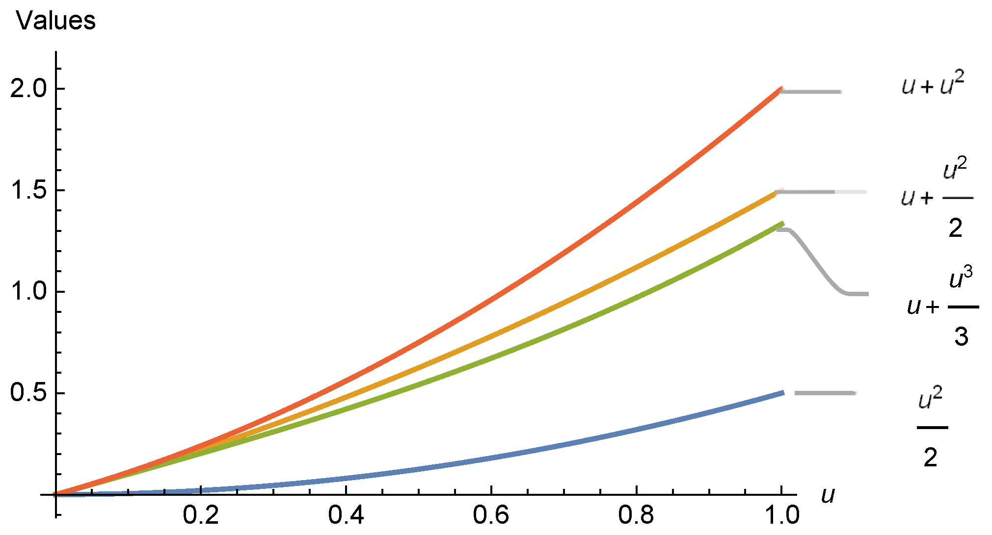
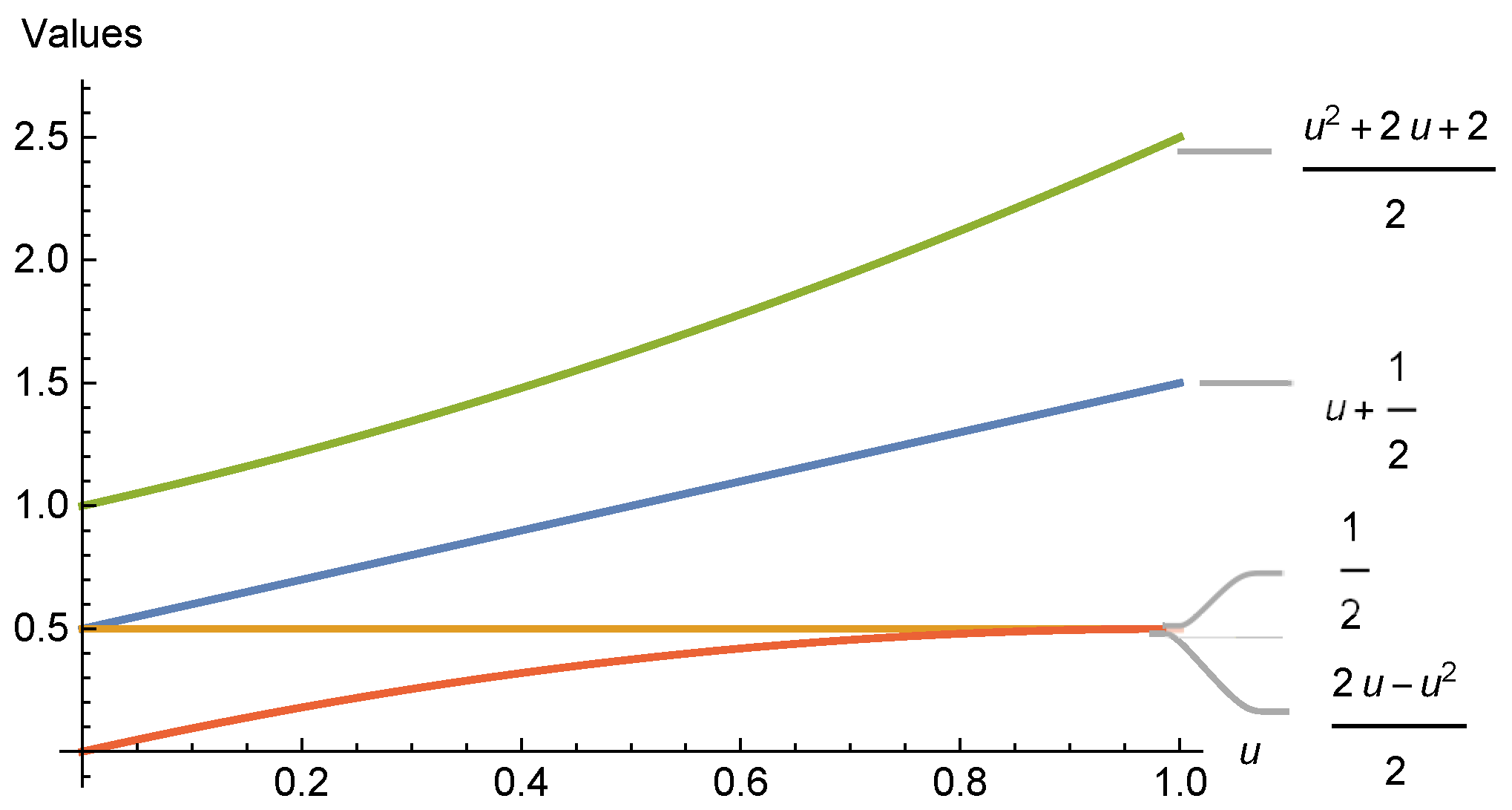
4. Numerical Estimations

Example 2.

Let $\mathcal{K}\left(\mathtt{u}\right)=[-{\mathtt{u}}^2+1,{\mathtt{u}}^2+2]$, $\psi (\mathit{s},\mathit{g})=\mathit{s}-\mathit{g}$, $\mathit{g}=0$, and $\mathit{s}=1$. Then, for $\alpha =\frac{1}{2}$ and $\mathtt{h}(\ell )=\ell$, all assumptions of Theorem 4 are satisfied. We have

$$\begin{array}{cc}\hfill \frac{1}{\alpha \mathtt{h}\left(\frac{1}{2}\right)}\mathcal{K}\left(\mathit{g}+\frac{1}{2}\psi (\mathit{s},\mathit{g})\right)& \approx [3,9],\hfill \\ \hfill \frac{\Gamma \left(\alpha \right)}{{\left(\psi (\mathit{s},\mathit{g})\right)}^{\alpha }}\left[{\mathrm{I}}_{{(\mathit{g}+\psi (\mathit{s},\mathit{g}))}^{-}}^{\alpha }\mathcal{K}\left(\mathit{g}\right)+{\mathrm{I}}_{{\mathit{g}}^{+}}^{\alpha }\mathcal{K}(\mathit{g}+\psi (\mathit{s},\mathit{g}))\right]& \approx \left[\frac{4.75}{1.875},\frac{17.75}{1.875}\right]\hfill \end{array}$$

and

$$[\mathcal{K}\left(\mathit{g}\right)+\mathcal{K}(\mathit{g}+\psi (\mathit{s},\mathit{g}))]{\int }_0^1{\ell }^{\alpha -1}[\mathtt{h}(\ell )+\mathtt{h}(1-\ell )]d\ell \approx \left[2,10\right].$$

Consequently,

$$[3,9]{⪯}_{\mathrm{cr}}\left[\frac{4.75}{1.875},\frac{17.75}{1.875}\right]{⪯}_{\mathrm{cr}}[2,10].$$

This ultimately confirms the validity of Theorem 4.

Example 3.

Let $\mathcal{K}\left(\mathtt{u}\right)=[{\mathtt{u}}^2,{\mathtt{u}}^3+1]$, $\mathcal{G}\left(\mathtt{u}\right)=[-{\mathtt{u}}^2+1,{\mathtt{u}}^2+2]$, $\psi (\mathit{s},\mathit{g})=\mathit{s}-\mathit{g}$, $\mathit{g}=0$ and $\mathit{s}=1$. Then, for $\mathtt{h}(\ell )=\ell$ and $\alpha =\frac{1}{2}$ all assumptions of Theorem 5 are satisfied. Let us denote

$$\begin{array}{cc}\hfill & \frac{\Gamma \left(\alpha \right)}{{\left(\psi (\mathit{s},\mathit{g})\right)}^{\alpha }}\left[{\mathrm{I}}_{{(\mathit{g}+\psi (\mathit{s},\mathit{g}))}^{-}}^{\alpha }\mathcal{K}\left(\mathit{g}\right)\mathcal{G}\left(\mathit{g}\right)+{\mathrm{I}}_{{\mathit{g}}^{+}}^{\alpha }\mathcal{K}(\mathit{g}+\psi (\mathit{s},\mathit{g}))\mathcal{G}(\mathit{g}+\psi (\mathit{s},\mathit{g}))\right]\approx [0.43,12.78],\hfill \\ \hfill & \mathcal{M}(\mathit{g},\mathit{g}+\psi (\mathit{s},\mathit{g})){\int }_0^1{\ell }^{\alpha -1}[{\mathtt{h}}_1(\ell ){\mathtt{h}}_2(\ell )+{\mathtt{h}}_1(1-\ell ){\mathtt{h}}_2(1-\ell )]d\ell \hfill \\ \hfill & +\mathcal{N}(\mathit{g},\mathit{g}+\psi (\mathit{s},\mathit{g})){\int }_0^1{\ell }^{\alpha -1}[{\mathtt{h}}_1(\ell ){\mathtt{h}}_2(1-\ell )+{\mathtt{h}}_1(1-\ell ){\mathtt{h}}_2(\ell )]d\ell \approx \left[0.53,15.47\right].\hfill \end{array}$$

Thus, it can be easily seen that

$$[0.43,12.78]{⪯}_{\mathrm{cr}}\left[0.53,15.47\right].$$

This ultimately confirms the validity of Theorem 5.

Example 4.

Similarly, if we take all the assumptions of Example 3, then all the hypotheses in Theorem 6 are satisfied.

Example 5.

Let $\mathcal{K}\left(\mathtt{u}\right)=[{\mathtt{u}}^2,{\mathtt{u}}^3+1]$, $\psi (\mathit{s},\mathit{g})=\mathit{s}-\mathit{g}$, $\mathit{g}=0$, and $\mathit{s}=1$. Then, for $\mathtt{h}(\ell )=\ell$ and symmetric function $\mathcal{W}\left(\mathtt{u}\right)={\left(\frac{1}{2}-\mathtt{u}\right)}^2$, where $\mathtt{u}\in [0,1]$ is symmetric about $\frac{1}{2}$, we have

$$\begin{array}{cc}\hfill & \mathcal{K}\left(\mathit{g}+\frac{1}{2}\psi (\mathit{s},\mathit{g})\right)\frac{\Gamma \left(\alpha \right)}{{\left(\psi (\mathit{s},\mathit{g})\right)}^{\alpha }}\left[{\mathrm{I}}_{{\mathit{g}}^{+}}^{\alpha }\mathcal{W}(\mathit{g}+\psi (\mathit{s},\mathit{g}))+{\mathrm{I}}_{{(\mathit{g}+\psi (\mathit{s},\mathit{g}))}^{-}}^{\alpha }\mathcal{W}\left(\mathit{g}\right)\right]\approx \left[\frac{7}{60},\frac{21}{40}\right],\hfill \\ \hfill & 2\mathtt{h}\left(\frac{1}{2}\right)\frac{\Gamma \left(\alpha \right)}{{\left(\psi (\mathit{s},\mathit{g})\right)}^{\alpha }}\left[{\mathrm{I}}_{{\mathit{g}}^{+}}^{\alpha }\mathcal{K}(\mathit{g}+\psi (\mathit{s},\mathit{g}))\mathcal{W}(\mathit{g}+\psi (\mathit{s},\mathit{g}))+{\mathrm{I}}_{{(\mathit{g}+\psi (\mathit{s},\mathit{g}))}^{-}}^{\alpha }\mathcal{K}\left(\mathit{g}\right)\mathcal{W}\left(\mathit{g}\right)\right]\approx \left[0.20,0.65\right].\hfill \end{array}$$

Let $A=\left[\frac{7}{60},\frac{21}{40}\right]$, and $B=\left[0.20,0.65\right]$. Then, $A_{\mathrm{c}}\approx 0.32$ and $B_{\mathrm{c}}\approx 0.42$. Thus, from Definition 2, it can be easily seen that

$$\left[\frac{7}{60},\frac{21}{40}\right]{⪯}_{\mathrm{cr}}\left[0.20,0.65\right].$$

This ultimately confirms the validity of Theorem 7.

Example 6.

Similarly, if we take all the assumptions of Example 5, then all the hypotheses in Theorem 8 are satisfied.

5. Conclusions

A suitable technique for introducing uncertainty into prediction processes is to use interval-valued functions. Using a new idea from [43], we proved fractional versions of the Hermite–Hadamard-, Fejér-, and Pachpatte-type inequalities. We demonstrated that our findings can generate a few novel findings for the $\mathrm{cr}-h$-convex function and h-preinvex functions.A new approach for $\mathrm{cr}$-ordered interval-valued inequalities involving the well-known Riemann–Liouville fractional integral was introduced. For clarification of the results, some numerical examples were studied as well. In the future, this approach can also be generalized for other fractional operators such as Atangana–Baleanu, Caputo–Fabrizio, tempered, generalized fractional integral operators, etc. Furthermore, this methodology can also be applied to various non-symmetric functions.

This innovative concept can be applied to future presentations of various inequalities, such as those of the Hermite–Hadamard, Ostrowski, Jensen–Mercer, Bullen, and Simpson types. These inequalities can also be established for a variety of interval-valued quantum calculus, fuzzy calculus, and fractional calculus.

References

1. Hadamard, J. Étude sur les propriétés des fonctions entiéres en particulier d’une fonction considéréé par Riemann. J. Math. Pures Appl. 1893, 58, 171–215. [Google Scholar]
2. Sarikaya, M.Z.; Set, E.; Yaldiz, H.; Başak, N. Hermite–Hadamard inequalities for fractional integrals and related fractional inequalities. Math. Comput. Model. 2013, 57, 2403–2407. [Google Scholar] [CrossRef]
3. Podlubny, I. Geometric and physical interpretations of fractional integration and differentiation. Fract. Calc. Appl. Anal. 2001, 5, 230–237. [Google Scholar]
4. Dragomir, S.S. Ostrowski type inequalities for Riemann-Liouville fractional integrals of absolutely continuous functions in terms of norms. RGMIA Res. Rep. Collect. 2017, 20, 49. [Google Scholar]
5. Set, E.; Akdemir, A.O.; Özdemir, M.E. Simpson type integral inequalities for convex functions via Riemann–Liouville integrals. Filomat 2017, 31, 4415–4420. [Google Scholar] [CrossRef]
6. Öğülmüs, H.; Sarikaya, M.Z. Hermite–Hadamard-Mercer type inequalities for fractional integrals. Filomat 2021, 35, 2425–2436. [Google Scholar] [CrossRef]
7. Chen, H.; Katugampola, U.N. Hermite–Hadamard and Hermite–Hadamard–Fejér type inequalities for generalized fractional integrals. J. Math. Anal. Appl. 2017, 446, 1274–1291. [Google Scholar] [CrossRef] [Green Version]
8. Fernandez, A.; Mohammed, P.O. Hermite-Hadamard inequalities in fractional calculus defined using Mittag-Leffler. kernels. Math. Methods Appl. Sci. 2020, 44, 8414–8431. [Google Scholar] [CrossRef]
9. Tariq, M.; Ahmad, H.; Sahoo, S.K.; Kashuri, A.; Nofal, T.A.; Hsu, C.H. Inequalities of Simpson-Mercer-type including Atangana-Baleanu fractional operators and their applications. AIMS Math. 2022, 7, 15159–15181. [Google Scholar] [CrossRef]
10. Gürbüz, M.; Akdemir, A.O.; Rashid, S.; Set, E. Hermite–Hadamard inequality for fractional integrals of Caputo-Fabrizio type and related inequalities. J. Inequl. Appl. 2020, 2020, 172. [Google Scholar] [CrossRef]
11. Sahoo, S.K.; Mohammed, P.O.; Kodamasingh, B.; Tariq, M.; Hamed, Y.S. New fractional integral inequalities for convex functions pertaining to Caputo-Fabrizio operator. Fractal Fract. 2022, 6, 171. [Google Scholar] [CrossRef]
12. Butt, S.I.; Agarwal, P.; Yousaf, S.; Guirao, J.L. Generalized fractal Jensen and Jensen–Mercer inequalities for harmonic convex function with applications. J. Inequal. Appl. 2022, 2022, 1. [Google Scholar] [CrossRef]
13. Sahoo, S.K.; Agarwal, R.P.; Mohammed, P.O.; Kodamasingh, B.; Nonlaopon, K.; Abualnaja, K.M. Hadamard–Mercer, Dragomir–Agarwal–Mercer, and Pachpatte–Mercer Type Fractional Inclusions for Convex Functions with an Exponential Kernel and Their Applications. Symmetry 2022, 14, 836. [Google Scholar] [CrossRef]
14. Butt, S.I.; Yousaf, S.; Khan, K.A.; Matendo Mabela, R.; Alsharif, A.M. Fejer–Pachpatte–Mercer-Type Inequalities for Harmonically Convex Functions Involving Exponential Function in Kernel. Math. Prob. Eng. 2022, 2022, 7269033. [Google Scholar] [CrossRef]
15. Srivastava, H.M.; Sahoo, S.K.; Mohammed, P.O.; Kodamasingh, B.; Hamed, Y.S. New Riemann–Liouville Fractional-Order Inclusions for Convex Functions via Interval-Valued Settings Associated with Pseudo-Order Relations. Fractal Fract. 2022, 6, 212. [Google Scholar] [CrossRef]
16. Bin-Mohsin, B.; Rafique, S.; Cesarano, C.; Javed, M.Z.; Awan, M.U.; Kashuri, A.; Noor, M.A. Some General Fractional Integral Inequalities Involving LR–Bi-Convex Fuzzy Interval-Valued Functions. Fractal Fract. 2022, 6, 565. [Google Scholar] [CrossRef]
17. Kashuri, A.; Samraiz, M.; Rahman, G.; Khan, Z.A. Some New Beesack–Wirtinger-Type Inequalities Pertaining to Different Kinds of Convex Functions. Mathematics 2022, 10, 757. [Google Scholar] [CrossRef]
18. Almutairi, O.; Kılıçman, A. A Review of Hermite–Hadamard Inequality for α-Type Real-Valued Convex Functions. Symmetry 2022, 14, 840. [Google Scholar] [CrossRef]
19. Xu, P.; Butt, S.I.; Ain, Q.U.; Budak, H. New Estimates for Hermite-Hadamard Inequality in Quantum Calculus via (α, m) Convexity. Symmetry 2022, 14, 1394. [Google Scholar] [CrossRef]
20. Yanagi, K. Refined Hermite-Hadamard Inequalities and Some Norm Inequalities. Symmetry 2022, 14, 2522. [Google Scholar] [CrossRef]
21. Markov, S. Calculus for interval functions of a real variable. Computing 1979, 22, 325–337. [Google Scholar] [CrossRef]
22. Shi, F.; Ye, G.; Liu, W.; Zhao, D. cr-h-convexity and some inequalities for cr-h-convex function. Filomat, 2022; submitted. [Google Scholar]
23. Bhunia, A.; Samanta, S. A study of interval metric and its application in multi-objective optimization with interval objectives. Comput. Ind. Eng. 2014, 74, 169–178. [Google Scholar] [CrossRef]
24. Moore, R.E. Interval Analysis; Prentice-Hall: Englewood Cliffs, NJ, USA, 1966. [Google Scholar]
25. Kulish, U.; Miranker, W. Computer Arithmetic in Theory and Practice; Academic Press: New York, NY, USA, 2014. [Google Scholar]
26. Zhang, D.; Guo, C.; Chen, D.; Wang, G. Jensen’s inequalities for set-valued and fuzzy set-valued functions. Fuzzy Sets Syst. 2020, 404, 178–204. [Google Scholar] [CrossRef]
27. Costa, T.M. Jensen’s inequality type integral for fuzzy-interval-valued functions. Fuzzy Sets Syst. 2017, 327, 31–47. [Google Scholar] [CrossRef]
28. Chalco-Cano, Y.; Lodwick, W.A. Condori-Equice. Ostrowski type inequalities and applications in numerical integration for interval-valued functions. Soft Comput. 2015, 19, 3293–3300. [Google Scholar] [CrossRef]
29. Román-Flores, H.; Chalco-Cano, Y.; Lodwick, W.A. Some integral inequalities for interval-valued functions. Comput. Appl. Math. 2018, 37, 1306–1318. [Google Scholar]
30. Costa, T.M.; Román-Flores, H.; Chalco-Cano, Y. Opial-type inequalities for interval-valued functions. Fuzzy Set. Syst. 2019, 358, 48–63. [Google Scholar] [CrossRef]
31. Zhao, D.F.; An, T.Q.; Ye, G.J.; Liu, W. New Jensen and Hermite-Hadamard type inequalities for h-convex interval-valued functions. J. Inequal. Appl. 2018, 2018, 302. [Google Scholar] [CrossRef] [Green Version]
32. An, Y.R.; Ye, G.J.; Zhao, D.F.; Liu, W. Hermite-Hadamard Type Inequalities for Interval (h1, h2)-Convex Functions. Mathematics 2019, 7, 436. [Google Scholar] [CrossRef] [Green Version]
33. Zhao, D.; Ali, M.A.; Murtaza, G.; Zhang, Z. On the Hermite-Hadamard inequalities for interval-valued coordinated convex functions. Adv. Differ. Equ. 2020, 2020, 570. [Google Scholar] [CrossRef]
34. Nwaeze, E.R.; Khan, M.A.; Chu, Y.M. Fractional inclusions of the Hermite-Hadamard type for m-polynomial convex interval-valued functions. Adv. Differ. Equ. 2020, 2020, 507. [Google Scholar] [CrossRef]
35. Sharma, N.; Singh, S.K.; Mishra, S.K.; Hamdi, A. Hermite-Hadamard type inequalities for interval-valued preinvex functions via Riemann-Liouville fractional integrals. J. Inequal. Appl. 2021, 2021, 98. [Google Scholar] [CrossRef]
36. Srivastava, H.M.; Sahoo, S.K.; Mohammed, P.O.; Baleanu, D.; Kodamasingh, B. Hermite-Hadamard type inequalities for interval-valued preinvex functions via fractional integral operators. Int. J. Comput. Intel. Syst. 2022, 15, 8. [Google Scholar] [CrossRef]
37. Lai, K.K.; Bisht, J.; Sharma, N.; Mishra, S.K. Hermite-Hadamard-Type Fractional Inclusions for Interval-Valued Preinvex Functions. Mathematics 2022, 10, 264. [Google Scholar] [CrossRef]
38. Hanson, M.A. On sufficiency of the Kuhn-Tucker conditions. J. Math. Anal. Appl. 1981, 80, 545–550. [Google Scholar] [CrossRef] [Green Version]
39. Ben-Isreal, A.; Mond, B. What is invexity? J. Aust. Math. Soc. Ser. B 1986, 28, 1–9. [Google Scholar] [CrossRef] [Green Version]
40. Weir, T.; Mond, B. Preinvex functions in multiple objective optimization. J. Math. Anal. Appl. 1988, 136, 29–38. [Google Scholar] [CrossRef] [Green Version]
41. Mohan, S.R.; Neogy, S.K. On invex sets and preinvex functions. J. Math. Anal. Appl. 1995, 189, 901–908. [Google Scholar] [CrossRef] [Green Version]
42. Matłoka, M. Inequalities for h-preinvex functions. Appl. Math. Comput. 2014, 234, 52–57. [Google Scholar] [CrossRef]
43. Sahoo, S.K.; Latif, M.A.; Alsalami, O.M.; Treanţă, S.; Sudsutad, W.; Kongson, J. Hermite–Hadamard, Fejér and Pachpatte-Type Integral Inequalities for Center-Radius Order Interval-Valued Preinvex Functions. Fractal Fract. 2022, 6, 506. [Google Scholar] [CrossRef]
Figure 1. Graphical validation of Theorem 1.
Axioms 11 00732 g001
Figure 2. The graph of K c = u + 1 2 , K r = 1 2 , G c = u 2 + 2 u + 2 2 and G r = 2 u u 2 2 .
Axioms 11 00732 g002
Publisher’s Note: MDPI stays neutral with regard to jurisdictional claims in published maps and institutional affiliations.