
A Fresh Approach to a Special Type of the Luria–Delbrück Distribution
Department of Epidemiology and Biostatistics, School of Public Health, Texas A&M University, College Station, TX 77843, USA
Axioms 2022, 11(12), 730; https://doi.org/10.3390/axioms11120730
Submission received: 19 October 2022
/
Revised: 29 November 2022
/
Accepted: 9 December 2022
/
Published: 14 December 2022
(This article belongs to the Special Issue Mathematics, Statistics, and Computation Inspired by the Fluctuation Test: In Celebration of the 80th Anniversary of the Luria-Delbrück Experiment)
Abstract
:The mutant distribution that accommodates both fitness and plating efficiency is an important class of the Luria–Delbrück distribution. Practical algorithms for computing this distribution do not coincide with the theoretically most elegant ones, as existing generic methods often either produce unreliable results or freeze the computational process altogether when employed to solve real-world research problems. Exploiting properties of the hypergeometric function, this paper offers an algorithm that considerably expands the scope of application of this important class of the Luria–Delbrück distribution. An integration method is also devised to complement the novel algorithm. Asymptotic properties of the mutant probability are derived to help gauge the new algorithm. An illustrative example and simulation results provide further guidelines on the use of the new algorithm.
MSC:
92D15; 92D25; 62M15; 33C901. Introduction
The first distribution in the Luria–Delbrück (LD) distribution family was proposed by Delbrück [1] to provide a mathematical foundation for a trailblazing experimental protocol proposed by Luria. Their joint paper, now a classic in genetics research, ushered in an 80-year period of relentless progress in the experimental determination of microbial mutation rates. The experimental protocol is variously referred to as the fluctuation test, the fluctuation experiment, or the Luria–Delbrück experiment. The data generated by such an experiment are called fluctuation assay data, which is a sequence of nonnegative integers representing the numbers of mutants found by the experimentalist in a series of cultures. (For details about the experimental protocol, see Ref. [2].) Today, despite rapid advances in sequencing technology, the LD experimental protocol remains a widely favored tool for studying microbial mutation rates in the laboratory. While there has been little alteration to the experimental protocol, the LD distribution family has been augmented considerably.
The first addition to the LD distribution family was made by Lea and Coulson [3] to overcome an important drawback of the distribution proposed by Delbrück. Note that Delbrück used a continuous distribution to model the number of bacterial mutants observed in Luria’s experiments. However, the numbers of mutants in those experiments were small random numbers, and they rarely exceeded 1000. Seeing that a continuous distribution was not an efficient tool to model the number of mutants, Lea and Coulson employed a stochastic birth process to construct a new discrete distribution. The distribution constructed by Lea and Coulson is uniquely determined by a single parameter m, which is the expected number of mutations. Lea and Coulson defined their new distribution by giving the probability generating function of the form
along with its more compact form (see Equation (15) in Ref. [3]). This distribution is now widely referred to as the Luria–Delbrück distribution mainly due to historical reasons, as the original distribution proposed by Delbrück fell into disuse soon after the work of Lea and Coulson.
Further augmentation of the LD distribution family was effected by laboratory needs and theoretical considerations. Mandelbrot [4] and Koch [5] independently extended the Lea–Coulson distribution to accommodate distinctive cell growth rates between mutants and nonmutants. The resulting distribution has a fitness parameter w, which is the ratio of the mutant growth rate to the nonmutant growth rate. Another driving force in the augmentation of the LD distribution is the fact that the number of mutants in a culture is often too large to count. This laboratory difficulty clamors for the study of distributions having a plating efficiency parameter that indicates how large a portion of each culture is actually plated to ease the counting burden. After a brief initial study of this kind of distribution by Armitage ([6], p. 14), several investigators explored these distributions more thoroughly in the 1990s [7,8,9,10,11]. More recently, further impetus for augmenting the LD distribution family comes from work on mathematical modeling of tumor progression. Antal and Krapivsky [12] studied the joint distribution of the numbers of both mutants and nonmutants. They allowed not only distinct cell growth rates between mutants and nonmutants, but also distinct cell death rates for both types of cells. In addition, Kessler and Levine [13] proposed a unified approach for computing mutant probabilities.
Efficient algorithms for computing various LD distributions are key to meaningful inference of microbial mutation rates. An algorithm must satisfy two practical requirements to be useful in the analysis of fluctuation assay data. First, it should remain operational for a wide range of key parameter values that an experimentalist might encounter in the laboratory. Among such parameters are and . Second, it should be capable of computing (the probability of k mutants) reasonably fast for for some meaningful K (e.g., K = 2000). In the past 30 years, an idea introduced by Ma et al. [14] to compute the Lea–Coulson distribution has served as the backbone of several algorithms for computing a variety of extensions of the Lea–Coulson distribution. In 2013, Kessler and Levine [15] outlined a new, unified approach that relied on numerical integration to compute a much wider class of LD distributions. More details were given later by the same authors [13]. Mazoyer et al. [16] employed a possibly similar integration-based approach to compute a wide assortment of LD distributions in the R package flan. For the most part, the implementation in flan achieved impressive accuracy and computing speed. However, there are situations where this universal approach may not be optimal, convenient, or practical, as shown by the following example.
This example was inspired by an inquiry from a yeast microbiologist. Her group was planning fluctuation experiments to measure the rate of extra-chromosome loss in yeast cells. Due to the high rates of extra-chromosome loss seen in a pilot study, these investigators would like to plate a 0.5% portion of each culture. They also planned to measure cell growth rates to help enhance the accuracy of their rate estimates. Clearly, their data would require an LD distribution involving and . Because , it is sensible to set as a testing value to allow a manageable number of mutants to be observed in the plated portion of a culture. Next, a value for the fitness parameter w is needed. Meaningful values for w lie around , and we here regard all real numbers on the interval as values for w that may be encountered in real-world research. To produce a complete testing example, we set . With this testing example, the latest version of flan (v. 0.9) can compute easily for . However, computing for any would cause flan to stop responding. Perhaps such an annoying problem can be circumvented by tweaking the algorithm on a case-by-case basis. Still, it is worthwhile to seek alternative algorithms to compute this special type of three-parameter LD distributions. In this paper, we offer a more practical algorithm for the three-parameter LD distribution that is crucial to the yeast microbiologist’s investigation and to numerous other investigations. We begin by studying this distribution’s probability generating function.
2. The Probability Generating Function
As just mentioned, sometimes a culture may contain too many mutants for the experimentalist to count. A way of overcoming this difficulty is to count mutants in only a fraction of the whole culture, a practice called partial plating. If an portion of the whole culture is taken (plated, in microbiology parlance) to count mutants, it is conceptually equivalent to subjecting all mutants in the whole culture to a binomial sampling process with the success probability being . (The parameter is called the plating efficiency). Therefore, the distribution of the number of mutants observed by the experimentalist is related to the distribution of the number of mutants in the whole culture. Armitage ([6], Equation (50)) gave the relation in terms of the two distributions’ generating functions as follows.
Here, and are respectively the generating functions of the number of mutants in the whole culture and of the number of mutants in the plated culture, and is the plating efficiency. A brief proof of Equation (1) may run as follows.
Let X be the number of mutants in the whole culture, and let Y be the number of mutants in the plated culture. From elementary theory of conditional probability it follows that
Therefore,
Now the distribution to be investigated can be assembled by using (1). The distribution of the number of mutants in the whole culture is the same distribution studied by Mandelbrot [4] and Koch [5]. This distribution is known [17] to have an approximate generating function of the form
where denotes the beta function. However, an equivalent expression due to Kessler and Levine [13] would facilitate subsequent development. Setting the two cell death rates to zero and adopting new notation, we reduce Equation (45) of Kessler and Levine [13] to
Here, the symbol is simplified notation for , which denotes the hypergeometric function as defined in Ref. [18], p. 238. Note that the generating function in (5) is well-defined for . The adoption of the hypergeometric function to help manipulate the generating function in (4) has caused the generating function to lose its definition at , as is clearly undefined at . However, this small price paid for mathematical convenience does not compromise the ensuing development. Combining (1) with (5) and simplifying, we obtain the desired generating function of the form
with
3. An Integration-Based Method
Let be the probability of k mutants. That is, . Here, we use the notation to denote the coefficient of in the Maclaurin series expansion of . The integration method is based on Cauchy’s integral formula for derivatives:
Note that is the pgf in (6) and is a circle around the origin with a radius smaller than one. By definition, for any given , the above integral can be computed by
where . However, in practice, there are important drawbacks to this idea. First, the integrand is a complex-valued function, which makes implementation and computation needlessly complicated. Second, it is not clear how to choose an appropriate value of r for a given problem, as a poorly chosen value of r can lead to a nonsensical result. Kessler and Levine [13] proposed a clever way of deforming the integration contour to overcome these difficulties. In this section, we adapt their strategy to devise an improved integration-based algorithm for computing .
The basic idea of Kessler and Levine was to transform the complex integral in (8) to a real integral along the positive real axis. One way to accomplish this task is to deform the contour into a new contour as depicted in Figure 1, which has previously been done in Ref. [19]. We first transform the integral in (8) to a real integral along the ray . To facilitate the transformation, we rewrite the hypergeometric function appearing in the pgf in (6). Applying the transform via Equation (9.5.9) in Ref. [18], we obtain
Note that the hypergeometric function appearing in the first term on the right-hand side of (9) will invalidate this transform when for , because is undefined for . This kind of drawback of the integration approach has been noticed in a previous study [19]. The practical implications of this drawback are worth noting. For example, when , the integration-based algorithm fails altogether. Moreover, for values of w close to 0.5, the algorithm may produce unreliable results. Nevertheless, the transform in (9), introduced to the study of the Luria–Delbrück distribution by Kessler and Levine [13], simplifies the integral in (8) in two important ways. First, for , Therefore, the hypergeometric function appearing in the first term on the right-hand side of (9) is a single-valued function of z for z on both edges of the ray . Second, because for all z, the second term on the right-hand side of (9) does not involve the hypergeometric function; but it can be a multivalued function, depending on whether z lies on the upper edge or lower edge of the ray. Therefore, we now focus on the second term on the right-hand side of (9) with the hypergeometric function removed.
For z on the upper and lower edges of the the ray , which are labeled and , respectively, in Figure 1, we have
Therefore, it follows that
Exponentiating (11) and then taking the imaginary part, we find that one factor of the integrand is
More precisely, is the imaginary part of the quantity in (11) when z lives on the upper edge of the ray ]. If z is on the lower edge of the ray, the imaginary part of (11) is .
In light of (9), the other factor of the integrand is
It is now necessary to assume that the integral along the small circle and that long the large circle vanish as and . As shown in Ref. [19], this kind of claim requires excessive amounts of tedious mathematics to prove, and we do not attempt to prove the two claims here. Assuming the validity of these two claims, we add the integrals on and to obtain
Following Kessler and Levine [13], we recast the above to an integral on the entire positive real axis:
where
Note that the expressions for and are expressible as
and
4. A More Practical Algorithm
Unlike the preceding strategy that extracts directly from the generating function , the strategy here focuses on the expansion of after recasting the generating function as . The success of this strategy relies on an obscure property of the exponential function. Let and be functions analytic inside the unit circle. Let and . Assume further that . Then the sequence can be determined by the sequence as follows.
Equation (17) can be established by differentiating the identity and then equating the coefficients for each separate power of z. This helpful relation can be traced to a once-popular calculus textbook published in the 1950s ([20], p. 448). In 1992, Ma et al. [14] used it to compute the Lea–Coulson distribution.
It follows from (6) that the generating function can be viewed as with
A straightforward way to compute the sequence is to regard as a composite function
with
The sequence can then be obtained by Faà di Bruno’s formula [21]. Theoretically, it seems an easy task. First, applying the Leibniz rule to the function leads to
Therefore,
Second, note that
Hence, can be computed by
Third, the derivatives can be computed from the and sequences using Faà di Bruno’s formula (e.g., Equation (2.2) in Ref. [21]). Finally, note that and for we have . Despite its obvious educational value, this method is of limited use in practice. According to the results of this author’s computational experiments, the computation of by this method is prohibitively expensive when .
A more practical algorithm for computing can be devised by a novel route. Applying Pfaff’s formula (e.g., Equation (9.5.1) in Ref. [18]) yields
Therefore, we can rewrite the generating function in (6) as with
Applying the differentiation formula for the hypergeometric function, e.g., Equation (9.2.3) in Ref. [18], we have for
Clearly,
The computation of the sequence can be improved by noting that for
where
and
Furthermore, setting , we can also compute the sequence recursively.
The forgoing development gives the following recipe for computing for .
5. Asymptotic Behavior of the Mutant Probability
Knowledge of the asymptotic behavior of is of theoretical interest in its own right. Moreover, it plays a helpful role in testing computer implementations of algorithms for computing . A standard tool for fathoming the asymptotic behavior of is classical analysis that relies on so-called transfer theorems in the spirit of the Tauberian method. To seek an asymptotic expression for by this route, we first cite two existing results.
Proposition 1.
Let be a complex-valued function analytic in for some and . Assume that as in ,
for some constants K and α. If , then
On the other hand, if α is a nonnegative integer, then
Here, the symbol defines the close domain with and . This result is due to Flajolet and Odlyzko ([22], Corollary 2).
The second result has appeared in the classic text of Titchmarsh ([23], p. 226) as an exercise for students.
Proposition 2.
Assume that . As ,
In Proposition 2 as stated in Ref. [23], z approaches 1 only along the real axis within the unit circle. In the following informal process, we assume that (32) holds for inside some . This assumption requires the symbol in (32) to represent the analytic continuation of the hypergeometric function defined in the complex plane cut long the segment .
Now an intuitive derivation of the asymptotic behavior of can be executed. Begin with the function defined in (23). Note that
Therefore, in view of Proposion 2, as , for ,
Observe that (34) is equivalent to
Hence it follows from the relation that
Let . Then satisfies the condition . Applying Proposition 1 to and noting the identity , we obtain the relation
As the constant 1 in (35) has no effect on the asymptotic behavior of , we conclude that
The foregoing argument ceases to work when . However, the case has been tackled earlier by a slightly different approach [24], and the result is in agreement with (36):
It appears an elusive goal to translate the above intuitive argument into a formal mathematical proof of (36). A perspicacious reviewer has offered a refreshing, rigorous proof that makes ingenious use of elaborate probabilistic machinery. To help the reader focus on the essence of the probabilistic proof, we present separately two results that play an integral role in the proof but that may distract the reader from the main idea if not proved before the proof of (36). The first result is a special case of a theorem due to Borovkov ([25], p. 258).
Proposition 3.
Let be analytic in a region containing the unit disk. Then
If is a probability generating function, then because . Therefore, .
The next result is more elementary.
Proposition 4.
Let and be nonnegative continuous functions on . Let be a sequence of nonnegative discrete random variables. Assume that
- 1.
- for ;
- 2.
- as ;
- 3.
- there exists a sequence of positive constants such that and
Then
Proof.
Given , there exists such that implies
On the other hand, due to assumption 3, there exists such that
holds almost everywhere. Therefore, for ,
holds almost everywhere. Note that assumption 1 guarantees the existence of for . Taking expectations leads to
which is the desired conclusion. □
Now we proceed to present the probabilistic proof of (36). Consider the generating function in (4). Combining (1) and (4) leads to the generating function of interest
where
Let . Applying the usual binomial-expansion formula and collecting coefficients of , we have
Now, consider two real-valued functions defined on :
and
Observe that as (see, e.g., p. 15 of Ref. [18]). Write
where is a random variable following a negative binomial distribution with parameters and . Because can be viewed as the sum of independently and identically distributed random variables obeying the geometric distribution with parameter , it follows from the strong law of large numbers (see, e.g., p. 42 of Ref. [26]) that
Here, the symbol signifies convergence almost everywhere. Therefore,
For any , the random variable satisfies
Hence it follows from the dominated convergence theorem (see, e.g., p. 42 of Ref. [26]) and (40) that
Clearly, satisfies assumption 1 in Proposition 4. Because , it follows that also satisfies assumption 1. Moreover, the random variable sequence satisfies assumption 3 in Proposition 4 with . In view of Proposition 4 and (41), (39) leads to
This is equivalent to (36) due to Proposition 3.
To show the usefulness of formula (36), we here employ it as a check on the recursive algorithm given in the preceding section. Consider cases where and . For and selected values of n, Table 1, Table 2 and Table 3 list exact values of computed by the recursive algorithm and their corresponding asymptotic values computed by formula (36). The relative errors, defined by , are shown in the last column.
6. Examples and Simulation Results
As alluded to earlier, the foregoing algorithms were motivated by an investigation on chromosome loss in yeast cells. The experimental context of this investigation is similar to that described in a previous study in Refs. [27,28]. In this experimental context, the colonies are the equivalent of the parallel cultures in a classic fluctuation experiment [28]. Table 4 and Table 5 give two fictitious data sets that mimic the real-world data to highlight several important features of such data. First, as reported by Wu et al. [28], there is high variation in , the final total number of viable cells in a culture. Second, there is also high variation in the plating efficiency . Due to these two challenging features, the mutation rate should be estimated directly, not via the estimation of m as is commonly practiced [2,29]. Therefore, the log likelihood function is
Here, is the number of mutants in the ith culture; and are respectively and for the ith culture. The experiment consists of n cultures and w is the fitness that is assumed to be constant cross all cultures (or colonies in the present context). The maximum likelihood (ML) estimator of , denoted by , is defined by
Many optimization algorithms can be employed to compute . The golden section search method ([30], p. 293) is one of the simplest methods for that purpose. The experimentalist starts the computational process by first bracketing the mutation rate via trial and error or by using prior knowledge. Furthermore, the log likelihood function in (42) can also be used to compute confidence intervals (CIs) for the mutation rates. Specifically, to compute the two boundary points of a CI for the mutation rate, we solve numerically the following equation:
Here, denotes the th quantile of the distribution with one degree of freedom. The bisection method ([30], p. 261) can be used to solve (44). The foregoing work extends previous research [31].
Assume that the unknown mutation rates in both fictitious experiments lie in the interval . Applying the above ideas to the first experiment yields a mutation rate estimate and a 95% likelihood ratio confidence interval . For the second experiment, the same method yields and a 95% likelihood ratio confidence interval .
Another essential task in microbial mutation research is the comparison of mutation rates under different conditions or between different strains. Let and be mutant data generated by two fluctuation experiments. In particular, the sample sizes are and respectively. Let the symbol and be corresponding values of the parameters and w associated with the mutant count data . Let the two mutation rates be and , respectively. Here, is assumed to be constant for all cultures in experiment , but this assumption can be relaxed without affecting the ensuing discussion.
The preferred method for comparing mutation rates in two independent fluctuation experiments is the likelihood ratio (LR) test [32]. To perform an LR test, we first compute ML estimates and separately using log likelihood functions and similarly defined as in (42). We next construct a combined log likelihood function
from which we compute a combined mutation rate estimate according to the definition
Finally, we compute an LR statistic using the definition
The test statistic asymptotically obeys a chi-squared distribution with one degree of freedom. Applying the LR test to the mutation rates in the two fictitious experiments, we obtain and .
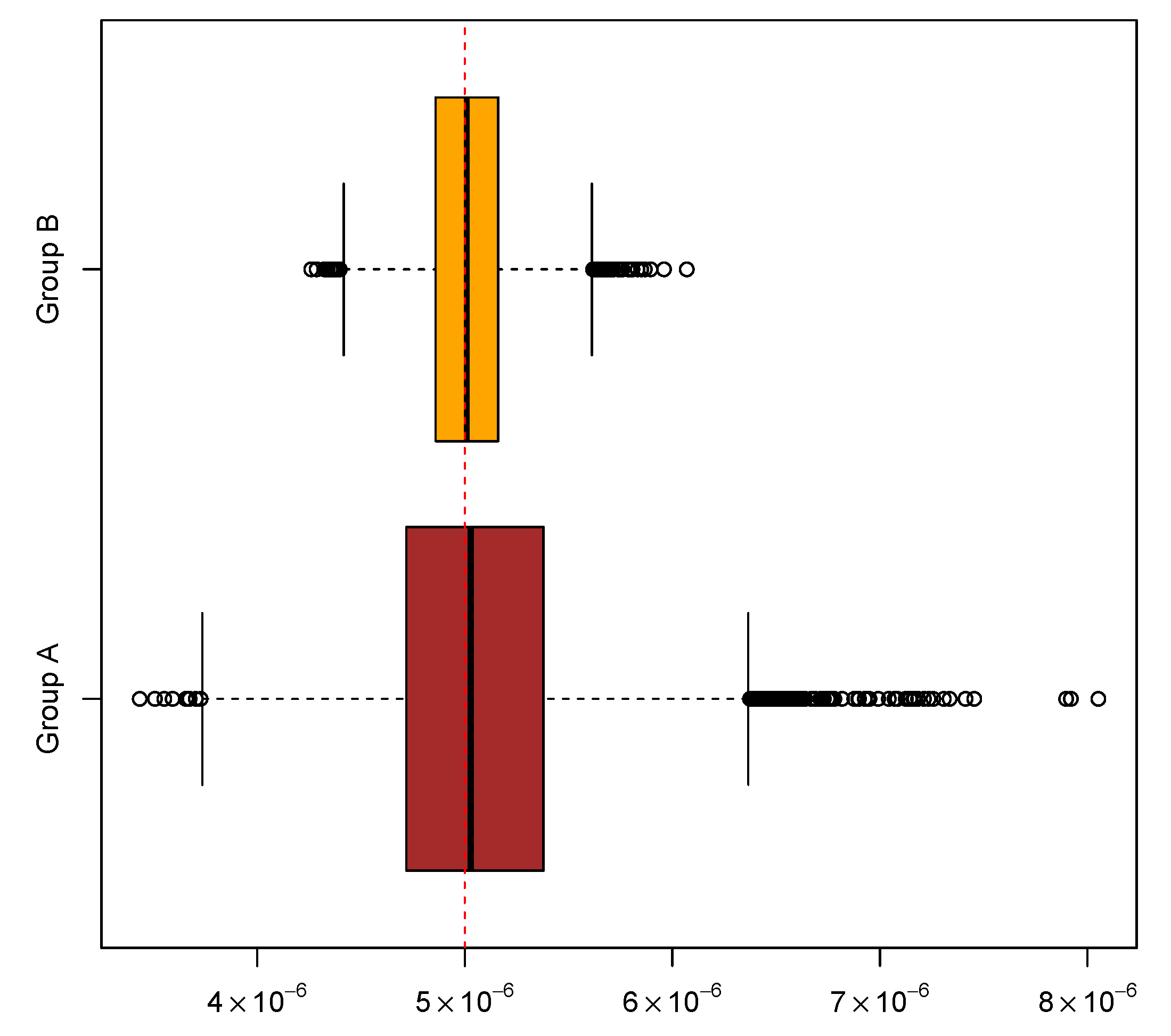
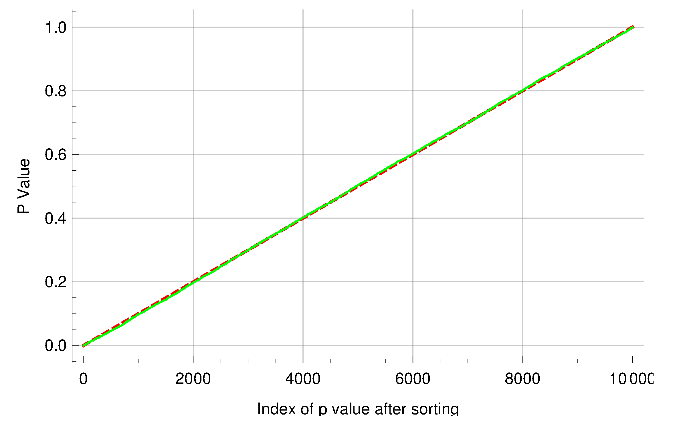
In addition, two groups of experiments were simulated to help assess the performance of the new algorithm. Each group comprises 10,000 experiments with a common mutation rate , and each experiment comprises 20 cultures. In the first group, the other parameter values were and ; in the second group, and . The above inference methods were applied to the two groups of simulated experiments to gauge the new algorithm for computing mutant distributions. The means and medians of the ML estimates and the coverage rates of the attendant 95% CIs are summarized in Table 6. The overall distributional patterns of the ML estimates are displayed in Figure 2. Moreover, experiments in the two groups were paired by their indices and then the LR test was performed on each of the 10,000 pairs of experiments. The sorted p-values produced by the tests exhibited an expected linear pattern as shown in Figure 3. Among the p-values, 545 of them were below 0.05. These results indicate that the new algorithm performed satisfactorily in this simulation study.
7. Concluding Remarks
This paper raises an oft-overlooked issue in research on the Luria–Delbrück distribution. Pure mathematical elegance is sometimes incongruous with real-world problems. A practical solution to a complex problem may occasionally appear inelegant and cumbersome at first sight. A large proportion of fluctuation experiments will produce data that are more amenable to the seemingly complicated and inefficient recursive algorithm presented here than to the integration or other existing algorithms. Admittedly, no algorithm is infallible under all circumstances. Combinations of values of and k can be found that allow certain to baffle the new algorithm as well as the existing algorithms for the Luria–Delbrück distribution. Thus, caution is advisable in practice. Furthermore, a unified algorithm does not seem to be recommendable. If either or holds, practitioners should use the simpler, more efficient existing algorithms [17]. The present investigation may herald a new paradigm for the estimation of microbial mutation rates using the Luria–Delbrück protocol. The examples based on fictitious data show how variations in and can be accounted for simultaneously using the new algorithm. The new algorithm may catalyze the exploration of untrodden territories in microbial mutation research.
Funding
This research received no external funding.
Data Availability Statement
The Python scripts used to generate the results in this paper are available at https://eeeeeric.com/rSalvador/, accessed on 11 December 2022.
Acknowledgments
I am particularly fortunate in receiving from a conscientious reviewer a formal proof of a key result that had eluded me during the writing of the first draft. Extensive algorithm testing in this research relied crucially on the advanced computing resources provided by Texas A&M High Performance Research Computing.
Conflicts of Interest
The author declares no conflict of interest.
References
- Luria, S.E.; Delbrück, M. Mutations of bacteria from virus sensitivity to virus resistance. Genetics 1943, 28, 491–511. [Google Scholar] [CrossRef] [PubMed]
- Foster, P.L. Methods for determining spontaneous mutation rates. Methods Enzymol. 2006, 409, 195–213. [Google Scholar] [PubMed] [Green Version]
- Lea, E.A.; Coulson, C.A. The distribution of the numbers of mutants in bacterial populations. J. Genet. 1949, 49, 264–285. [Google Scholar] [CrossRef] [PubMed]
- Mandelbrot, B. A population birth-and-mutation process, I: Explicit distributions for the number of mutants in an old culture of bacteria. J. Appl. Probab. 1974, 11, 437–444. [Google Scholar] [CrossRef]
- Koch, A.L. Mutation and growth rates from Luria-Delbrück fluctuation tests. Mutat. Res. 1982, 95, 129–143. [Google Scholar] [CrossRef]
- Armitage, P. The statistical theory of bacterial population subject to mutation. J. R. Stat. Soc. Ser. B 1952, 14, 1–44. [Google Scholar] [CrossRef]
- Stewart, F.M.; Gordon, D.M.; Levin, B.R. Fluctuation analysis: The probability distribution of the number of mutants under different conditions. Genetics 1990, 124, 175–185. [Google Scholar] [CrossRef]
- Stewart, F.M. Fluctuation analysis: The effect of plating efficiency. Genetica 1991, 84, 51–55. [Google Scholar] [CrossRef]
- Jones, M.E. An algorithm accounting for plating efficiency in estimating spontaneous mutation rates. Comput. Biol. Med. 1993, 23, 455–461. [Google Scholar] [CrossRef]
- Jones, M.E. Luria–Delbrück fluctuation experiments; accounting simultaneously for plating efficiency and differential growth rate. J. Theor. Biol. 1994, 166, 355–563. [Google Scholar] [CrossRef]
- Jones, M.E.; Thomas, S.M.; Rogers, A. Luria–Delbrück fluctuation experiments: Design and analysis. Genetics 1994, 136, 1209–1216. [Google Scholar] [CrossRef] [PubMed]
- Antal, T.; Krapivsky, P.L. Exact solution of a two-type branching process: Models of tumor progression. J. Stat. Mech. Theory Exp. 2011, 2011, P08018. [Google Scholar] [CrossRef]
- Kessler, D.A.; Levine, H. Scaling solution in the large population limit of the general asymmetric stochastic Luria–Delbrück evolution process. J. Stat. Phys. 2015, 158, 783–805. [Google Scholar] [CrossRef] [Green Version]
- Ma, W.T.; vH Sandri, G.; Sarkar, S. Analysis of the Luria and Delbrück distribution using discrete convolution powers. J. Appl. Probab. 1992, 29, 255–267. [Google Scholar] [CrossRef]
- Kessler, D.A.; Levine, H. Large population solution of the stochastic Luria–Delbrück evolution model. Proc. Natl. Acad. Sci. USA 2013, 110, 11682–11687. [Google Scholar] [CrossRef] [Green Version]
- Mazoyer, A.; Drouilhet, R.; Despréaux, S.; Ycart, B. flan: An R Package for Inference on Mutation Models. R J. 2017, 9, 334–351. [Google Scholar] [CrossRef] [Green Version]
- Zheng, Q. A new practical guide to the Luria–Delbrück protocol. Mutat. Res. 2015, 781, 7–13. [Google Scholar] [CrossRef]
- Lebedev, N.N. Special Functions and Their Applications; Silverman, R.A., Translator; Dover Publications, Inc.: New York, NY, USA, 1972. [Google Scholar]
- Zheng, Q. Estimation of rates of non-neutral mutations when bacteria are exposed to subinhibitory levels of antibiotic. Bull. Math. Biol. 2022, 84, 131. [Google Scholar] [CrossRef]
- Fichtenholtz, G.M. Differential- und Integralrechnung; VEB Deutscher Verlag der Wissenschaften: Berlin, Germany, 1954; Volume 2. [Google Scholar]
- Johnson, W.P. The curious history of Faà di Bruno’s formula. Am. Math. Mon. 2002, 109, 217–234. [Google Scholar]
- Flajolet, P.; Odlyzko, A. Singularity analysis of generating functions. SIAM J. Disc. Math. 1990, 3, 216–240. [Google Scholar] [CrossRef] [Green Version]
- Titchmarsh, E.C. The Theory of Functions, 2nd ed.; Oxford University Press: London, UK, 1939. [Google Scholar]
- Zheng, Q. Remarks on the asymptotics of the Luria–Delbrück and related distributions. J. Appl. Probab. 2009, 46, 1221–1224. [Google Scholar] [CrossRef]
- Borovkov, A.A. Stochastic Processes in Queueing Theory; Springer: Berlin/Heidelberg, Germany, 1976. [Google Scholar]
- Chung, K.K. A Course in Probability Theory, 2nd ed.; Academic Press: Cambridge, MA, USA, 1974. [Google Scholar]
- Strome, E.D.; Wu, X.; Kimmel, M.; Plon, S.E. Heterozygous screen in Saccharomyces cerevisiae identified dosage-sensitive genes that affect chromosome stability. Genetics 2008, 178, 1193–1207. [Google Scholar] [CrossRef] [PubMed] [Green Version]
- Wu, X.; Strome, E.D.; Meng, Q.; Hastings, P.J.; Plon, S.E. A robust estimator of mutation rates. Mutat. Res. 2009, 661, 101–109. [Google Scholar] [CrossRef] [PubMed]
- Zheng, Q. New algorithms for Luria–Delbrück fluctuation analysis. Math. Biosci. 2005, 196, 198–214. [Google Scholar] [CrossRef] [PubMed]
- Press, W.H.; Flannery, B.P.; Teukolsdy, S.A.; Vetterlind, W.T. Numerical Recipes in C: The Art of Scientific Computing; Cambridge University Press: Cambridge, UK, 1988. [Google Scholar]
- Zheng, Q. A note on plating efficiency in fluctuation experiments. Math. Biosci. 2008, 216, 150–153. [Google Scholar] [CrossRef]
- Zheng, Q. Comparing mutation rates under the Luria–Delbrück protocol. Genetica 2016, 144, 351–359. [Google Scholar] [CrossRef] [PubMed]
Figure 1.
A contour used to derive the algorithm for computing given by (15).
Figure 1.
A contour used to derive the algorithm for computing given by (15).

Figure 2.
Distributional patterns of maximum likelihood estimates of mutation rates based on two groups of simulated experiments. Each group comprises 10,000 experiments simulated by assuming a common mutation rate of .
Figure 2.
Distributional patterns of maximum likelihood estimates of mutation rates based on two groups of simulated experiments. Each group comprises 10,000 experiments simulated by assuming a common mutation rate of .

Figure 3.
The p-values generated by performing likelihood ratio tests on 10,000 pairs of simulated fluctuation experiments. Because the two mutation rates were equal, the sorted p-values exhibited an expected linear pattern. The solid line represents the observed p-values, and the dashed line represents the theoretical reference lines with slope and y-intercept 0.


Table 1.
Comparison of exact and asymptotic . .
| k | Recursive | Asymptotic | Error |
|---|---|---|---|
| 1000 | 6.3946195 × 10 | 6.2485639 × 10 | 2.28% |
| 1200 | 4.6651675 × 10 | 4.5713128 × 10 | 2.01% |
| 1400 | 3.5743179 × 10 | 3.5097405 × 10 | 1.81% |
| 1600 | 2.8383575 × 10 | 2.7916453 × 10 | 1.65% |
| 1800 | 2.3163411 × 10 | 2.2812359 × 10 | 1.52% |
| 2000 | 1.9314605 × 10 | 1.9042712 × 10 | 1.41% |
| 2500 | 1.3147908 × 10 | 1.2989647 × 10 | 1.20% |
| 3000 | 9.6046479 × 10 | 9.5029417 × 10 | 1.06% |
| 3500 | 7.3661056 × 10 | 7.2961229 × 10 | 0.95% |
| 4000 | 5.8539548 × 10 | 5.8033314 × 10 | 0.86% |
| 4500 | 4.7803264 × 10 | 4.7422815 × 10 | 0.80% |
| 5000 | 3.9881054 × 10 | 3.9586392 × 10 | 0.74% |
| 5500 | 3.3853023 × 10 | 3.3619173 × 10 | 0.69% |
| 6000 | 2.9149900 × 10 | 2.8960539 × 10 | 0.65% |
| 7500 | 1.9865134 × 10 | 1.9754916 × 10 | 0.55% |
| 8000 | 1.7780098 × 10 | 1.7685851 × 10 | 0.53% |
| 8500 | 1.6021445 × 10 | 1.5940085 × 10 | 0.51% |
| 9000 | 1.4523093 × 10 | 1.4452265 × 10 | 0.49% |
| 9500 | 1.3235060 × 10 | 1.3172937 × 10 | 0.47% |
| 10,000 | 1.2118944 × 10 | 1.2064088 × 10 | 0.45% |
| 10,500 | 1.1144824 × 10 | 1.1096090 × 10 | 0.44% |
| 11,000 | 1.0289091 × 10 | 1.0245558 × 10 | 0.42% |
Table 2.
Comparison of exact and asymptotic . .
| k | Recursive | Asymptotic | Error |
|---|---|---|---|
| 1000 | 2.9574909 × 10 | 2.9350000 × 10 | 0.76% |
| 1200 | 2.0513796 × 10 | 2.0381944 × 10 | 0.64% |
| 1400 | 1.5058433 × 10 | 1.4974490 × 10 | 0.56% |
| 1600 | 1.1521612 × 10 | 1.1464844 × 10 | 0.49% |
| 1800 | 9.0988439 × 10 | 9.0586420 × 10 | 0.44% |
| 2000 | 7.3670246 × 10 | 7.3375000 × 10 | 0.40% |
| 2500 | 4.7113536 × 10 | 4.6960000 × 10 | 0.33% |
| 3000 | 3.2701091 × 10 | 3.2611111 × 10 | 0.28% |
| 3500 | 2.4016450 × 10 | 2.3959184 × 10 | 0.24% |
| 4000 | 1.8382465 × 10 | 1.8343750 × 10 | 0.21% |
| 4500 | 1.4521236 × 10 | 1.4493827 × 10 | 0.19% |
| 5000 | 1.1760123 × 10 | 1.1740000 × 10 | 0.17% |
| 5500 | 9.7176953 × 10 | 9.7024793 × 10 | 0.16% |
| 6000 | 8.1645662 × 10 | 8.1527778 × 10 | 0.14% |
| 7500 | 5.2239033 × 10 | 5.2177778 × 10 | 0.12% |
| 8000 | 4.5910062 × 10 | 4.5859375 × 10 | 0.11% |
| 8500 | 4.0665264 × 10 | 4.0622837 × 10 | 0.10% |
| 9000 | 3.6270442 × 10 | 3.6234568 × 10 | 0.10% |
| 9500 | 3.2551386 × 10 | 3.2520776 × 10 | 0.09% |
| 10,000 | 2.9376332 × 10 | 2.9350000 × 10 | 0.09% |
| 10,500 | 2.6644134 × 10 | 2.6621315 × 10 | 0.09% |
| 11,000 | 2.4276104 × 10 | 2.4256198 × 10 | 0.08% |
Table 3.
Comparison of exact and asymptotic . .
| k | Recursive | Asymptotic | Error |
|---|---|---|---|
| 1000 | 2.8496504 × 10 | 2.8380054 × 10 | 0.41% |
| 1200 | 1.8289321 × 10 | 1.8227030 × 10 | 0.34% |
| 1400 | 1.2571893 × 10 | 1.2535188 × 10 | 0.29% |
| 1600 | 9.0866594 × 10 | 9.0634442 × 10 | 0.26% |
| 1800 | 6.8242226 × 10 | 6.8087237 × 10 | 0.23% |
| 2000 | 5.2823729 × 10 | 5.2715748 × 10 | 0.20% |
| 2500 | 3.0711312 × 10 | 3.0661083 × 10 | 0.16% |
| 3000 | 1.9718894 × 10 | 1.9692016 × 10 | 0.14% |
| 3500 | 1.3558537 × 10 | 1.3542696 × 10 | 0.12% |
| 4000 | 9.8019343 × 10 | 9.7919126 × 10 | 0.10% |
| 4500 | 7.3626620 × 10 | 7.3559704 × 10 | 0.09% |
| 5000 | 5.6999368 × 10 | 5.6952742 × 10 | 0.08% |
| 5500 | 4.5218134 × 10 | 4.5184507 × 10 | 0.07% |
| 6000 | 3.6602731 × 10 | 3.6577779 × 10 | 0.07% |
| 7500 | 2.1286359 × 10 | 2.1274749 × 10 | 0.05% |
| 8000 | 1.8197713 × 10 | 1.8188408 × 10 | 0.05% |
| 8500 | 1.5705871 × 10 | 1.5698313 × 10 | 0.05% |
| 9000 | 1.3669876 × 10 | 1.3663663 × 10 | 0.05% |
| 9500 | 1.1987501 × 10 | 1.1982339 × 10 | 0.04% |
| 10,000 | 1.0583261 × 10 | 1.0578931 × 10 | 0.04% |
| 10,500 | 9.4005077 × 10 | 9.3968451 × 10 | 0.04% |
| 11,000 | 8.3961125 × 10 | 8.3929899 × 10 | 0.04% |
Table 4.
Fictitious data set A ().
| Mutant | ||
|---|---|---|
| 881,200 | 0.12 | 2 |
| 1,147,200 | 0.11 | 1 |
| 529,800 | 0.22 | 19 |
| 1,215,300 | 0.14 | 42 |
| 230,000 | 0.2 | 10 |
| 748,400 | 0.04 | 0 |
| 296,500 | 0.4 | 6 |
| 378,800 | 0.87 | 8 |
| 1,318,500 | 0.63 | 32 |
| 1,328,000 | 0.27 | 10 |
| 999,400 | 0.28 | 3 |
| 1,567,500 | 0.5 | 11 |
Table 5.
Fictitious data set B ().
| Mutant | ||
|---|---|---|
| 432,900 | 0.86 | 213 |
| 54,300 | 5.61 | 31 |
| 145,600 | 2.40 | 481 |
| 103,700 | 4.70 | 79 |
| 138,600 | 3.69 | 151 |
| 115,000 | 5.25 | 161 |
| 100,100 | 3.57 | 833 |
| 51,400 | 8.14 | 895 |
| 364,100 | 1.46 | 1262 |
| 118,800 | 3.93 | 899 |
Table 6.
Summary of algorithm performance.
| Group | Mean of | Median of | 95% CI Coverage |
|---|---|---|---|
| A | 5.071 × 10 | 5.029 × 10 | 94.75% |
| B | 5.010 × 10 | 5.001 × 10 | 95.30% |
Publisher’s Note: MDPI stays neutral with regard to jurisdictional claims in published maps and institutional affiliations. |
© 2022 by the author. Licensee MDPI, Basel, Switzerland. This article is an open access article distributed under the terms and conditions of the Creative Commons Attribution (CC BY) license (https://creativecommons.org/licenses/by/4.0/).
Share and Cite
MDPI and ACS Style
Zheng, Q. A Fresh Approach to a Special Type of the Luria–Delbrück Distribution. Axioms 2022, 11, 730. https://doi.org/10.3390/axioms11120730
AMA Style
Zheng Q. A Fresh Approach to a Special Type of the Luria–Delbrück Distribution. Axioms. 2022; 11(12):730. https://doi.org/10.3390/axioms11120730
Chicago/Turabian StyleZheng, Qi. 2022. "A Fresh Approach to a Special Type of the Luria–Delbrück Distribution" Axioms 11, no. 12: 730. https://doi.org/10.3390/axioms11120730
Note that from the first issue of 2016, this journal uses article numbers instead of page numbers. See further details here.