
Coincidence Theory of a Nonlinear Periodic Sturm–Liouville System and Its Applications


Department of Mathematics, School of Electronics & Information Engineering, Taizhou University, Taizhou 318000, China
Axioms 2022, 11(12), 726; https://doi.org/10.3390/axioms11120726
Submission received: 22 November 2022
/
Revised: 8 December 2022
/
Accepted: 10 December 2022
/
Published: 13 December 2022
(This article belongs to the Special Issue Differential Equations in Applied Mathematics)
Abstract
:Based on the second derivative, this paper directly establishes the coincidence degree theory of a nonlinear periodic Sturm–Liouville (SL) system. As applications, we study the existence of periodic solutions to the S–L system with some special nonlinear functions by applying Mawhin’s continuation theorem. Some examples and simulations are furnished to inspect the correctness and availability of the chief findings.
MSC:
34A34; 34K13; 54H251. Introduction
The S–L equation is one of the most important second-order ODEs, which includes famous physical equations such as the Helmholtz equation, Bessel equation and Legendre equation. Meanwhile, any second-order linear ODE can be transformed into the S–L equation by an appropriate transformation. Therefore, it is of great significance to reveal the various dynamic properties of S–L equation. This manuscript mainly considers the following nonlinear periodic S–L system:
where , , , and there is a constant such that , and , for all .
The S–L equation is a famous mathematical and physical equation with a history of more than 200 years. Many scholars have conducted extensive and in-depth research on it from aspects of theory and application, and have achieved fruitful results. However, we will not repeat the early research results of the S–L equation. We only review some of the latest research achievements and progress of the S–L equation in recent years. The latest research trends on the S–L equation mainly include the following aspects. The first involves the theoretical and numerical methods and applications of inverse S–L problems (see [1,2,3,4,5,6,7,8,9,10,11,12,13,14,15,16]). The second focuses on the investigation of some generalized S–L equations, such as the fractional differential S–L equation (see [13,14,15,17,18,19,20,21,22,23,24]) and the S–L equation on time scales (see [25,26,27,28,29,30,31,32,33,34]). The third deals with the S–L problems with certain singularity (see [35,36,37,38]) or discontinuity (see [11,12]).
This manuscript focuses on the following novel works: (a) We have established the coincidence degree theory for system (1) based on the second derivative. Since the zero-index Fredholm operator that we constructed involves the second derivative, it will be complex and difficult to construct the inverse operator of and projection operators . (b) For some special forms of , we employ Mawhin’s continuation theorem to prove that system (1) has a periodic positive solution. In addition, with the exception that is required to be a positive periodic function, other conditions for the existence of periodic solutions of (1) are not affected by . As far as we know, our research topics and findings have not been seen in previous papers. Therefore, our work expands the application scope of coincidence degree theory and tries a new research method for the S–L equation.
The remaining composition of the manuscript as follows. Section 2 mainly establishes the coincidence degree theory for the S–L system (1). In Section 3, we apply our coincidence degree theory to study the existence of periodic positive solutions for two kinds of special nonlinear S–L system. Section 4 provides some examples and simulations to examine the correctness of our results. In the last Section 5, we briefly summarize the problem and method of the paper, and offer a simple outlook for future research directions.
2. Preliminaries and Coincidence Theory of System (1)
In this section, we attempt to build the coincidence degree theory for system (1). To this end, the following concepts and lemmas are essential.
Let and be real Banach spaces, and define a linear operator and a continuous operator . is called a zero-index Fredholm operator iff , and is closed in . Assuming that is a zero-index Fredholm operator, then there are continuous projectors and such that , , and , , where is an identity operator. It infers that is invertible and its inverse is denoted by . Let be a bounded open set, if is bounded and is compact, then is called -compact on . Since and are isomorphic, there is an isomorphism . Furthermore, the below Mawhin continuation theorem [39] is extremely important in the subsequent discussion.
Lemma 1.
Ref. [39] For the given real Banach spaces , and a bounded open subset , let be a zero-index Fredholm operator, and an operator be -compact on . Assuming that
- (i)
- every solution of possesses ,
- (ii)
- ,
- (iii)
- .
- then has a solution in .
Let be equipped with the norm , then and are Banach spaces.
Lemma 2.
For a given with , define by
then is a zero-index Fredholm operator.
Proof.
Obviously, is linear. From and (2), one has
where c and d are arbitrary real constants. By and (3), one obtains
It follows from and (4) that , which implies that . Thus, . In addition, for any such that , there exists such that . Therefore, one has
which implies that . Thus, one concludes that , i.e., is closed in . So is a zero-index Fredholm operator. The proof is complete. □
Lemma 3.
Define the operators and by
Then, and are all continuous projectors such that
Proof.
It is easy to verify that and are all continuous. From (5), one has
which implies . Similarly, . Thus, one knows that and are all continuous projectors. For each , it follows from (5) that is a real constant, which indicates . For any constant , we have and . This leads to . So , and . For any , then and . Denote , then . Now, we solve to obtain
where are any real constants. Similar to (4), we derive from (6) that
Taking , we know from (6) and (7) that such that , which means that , that is, . Conversely, for each , there exists a such that . By , and (6), we obtain
Taking the derivative of two sides of (8) with respect to t, we apply to obtain
(9) means that , namely . Thus, , and . The proof is complete. □
From Lemmas 2 and 3, is invertible. Its inverse is given as follows.
Lemma 4.
For all , is defined by
where , and .
3. Existence of Periodic Solution
Section 2 has basically established the coincidence degree theory corresponding to system (1). As applications, this section stresses the existence of periodic solutions for (1) with and , where and . These two special forms of are derived from the ecosystem model. The former comes from the Gilpin–Ayala ecosystem; the latter comes from the Lotka–Volterra ecosystem. , and stand for the natural growth rate, intraspecific competition rate and artificial harvest of species, respectively. For convenience, we denote and , where is a continuous -periodic function.
Theorem 1.
In system (1), let . If the following conditions and hold, then system (1) contains at least one ϖ-periodic positive solution in .
- Assume that , , , and is a constant. Moreover, α, β, , and are ϖ-periodic functions.
- , , and .
Proof.
The proof of this assertion is mainly completed by applying Lemma 1. To do so, the operators , , and are defined by (2), (5) and (10) based on Lemmas 2–4. In addition, the operator is given by
Clearly, and are continuous. For any open-bounded subset of , we easily apply the Arzela–Ascoli theorem to show that is compact, and is bounded. Thus, is -compact on .
Consider an operator equation , i.e.,
If Equation (14) contains an -periodic solution , then there exist such that , , , and . Noticing that , it follows from that
Let , . According to and Lemma 2.2 in [40,41], we know that the unique minimum points of and are, respectively, given by
The minimums are
Since
we yield that , and there exist only four real constants , , and such that
From the expressions of and , , we have . Thus, we obtain . By (17) and (18), we obtain and . Noting that is strictly increasing in , leads to
Obviously, is open-bounded such that Lemma 1 is true.
Choosing as the identity operator, and noting that , a direct calculation gives
Thus, Lemma 1 is also true. It follows from Lemma 1 that system (1) has at least an -periodic positive solution satisfying . The proof is complete. □
Theorem 2.
In system (1), let . If the following conditions and hold, then system (1) contains at least one ϖ-periodic positive solution in .
- Assume that , , , and α, β, , and are ϖ-periodic functions.
- , .
Proof.
Similar to the proof of Theorem 1, the operators , , and are defined by (2), (5) and (10) based on Lemmas 2–4. In addition, the operator is given by
Clearly, and are continuous. For any open-bounded subset of , we easily apply the Arzela–Ascoli theorem to show that is compact, and is bounded. Thus, is -compact on .
Consider an operator equation , i.e.,
Assuming that Equation (22) has an -periodic solution , then there exist such that , , , and . Noticing that , we derive from that
Apparently, is open-bounded such that Lemma 1 holds. Additionally, ; we know from (24) and (25) that and . Thus, Lemma 1 holds.
Taking the identity operator , and noticing that , we have
Thus, Lemma 1 also holds. From Lemma 1, we conclude that system (1) has at least an -periodic positive solution satisfying . The proof is complete. □
4. Illustrative Examples and Simulations
Since Equation (1) is a second-order ODE, it is necessary to convert it into a system of first-order ODEs for numerical simulation. Let and , then, Equation (1) becomes
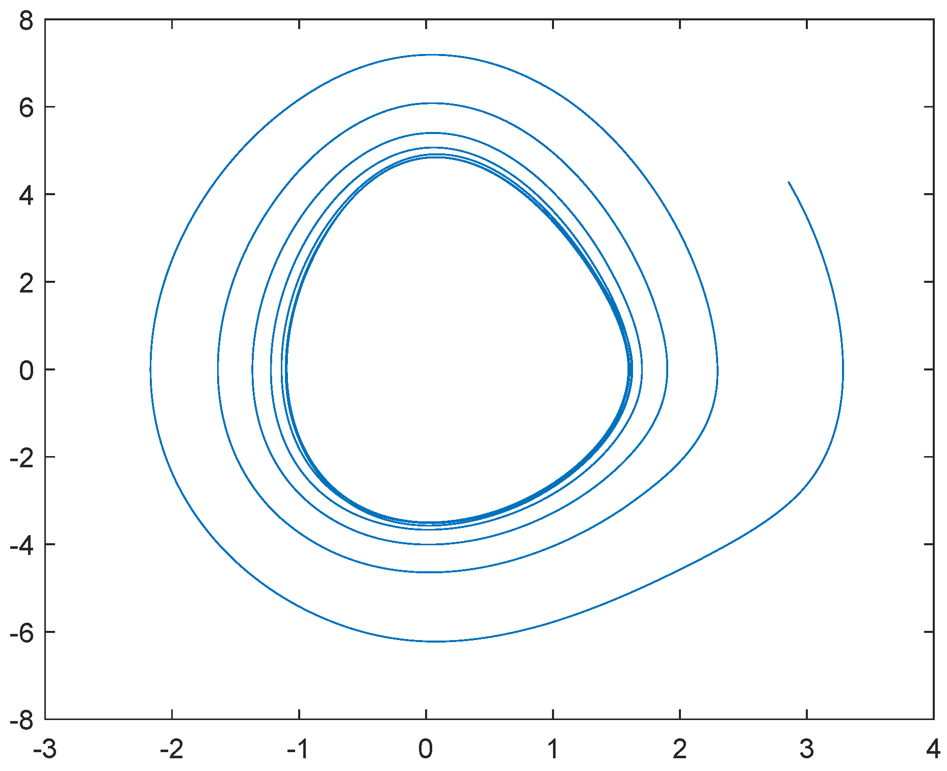
Example 1.
Consider the following ODE
where , , , , , .
Obviously, and the condition holds. By a simple calculation, we have , , , , , and . Therefore, the condition also holds. By solving the following algebraic equation
we obtain , , and . Thus,
Therefore, we conclude from Theorem 1 that (30) has at least a -periodic positive solution .
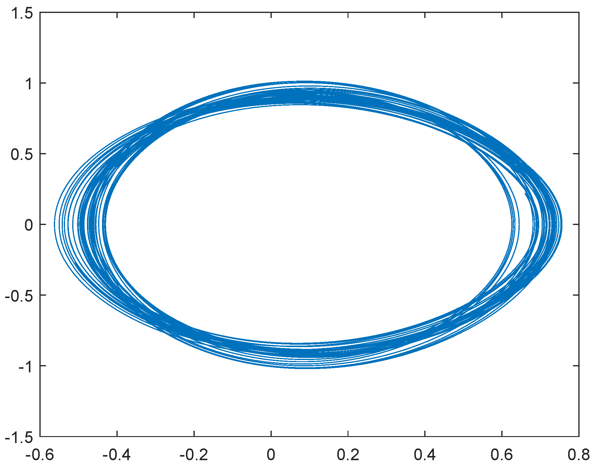
Example 2.
Consider the following ODE
where , , , , , .
Obviously, and the condition holds. We simply compute that , , , , , and . Therefore, the condition also holds. By solving the following algebraic equation
we obtain , , and . Thus,
Therefore, we conclude from Theorem 1 that (31) has at least a -periodic positive solution .
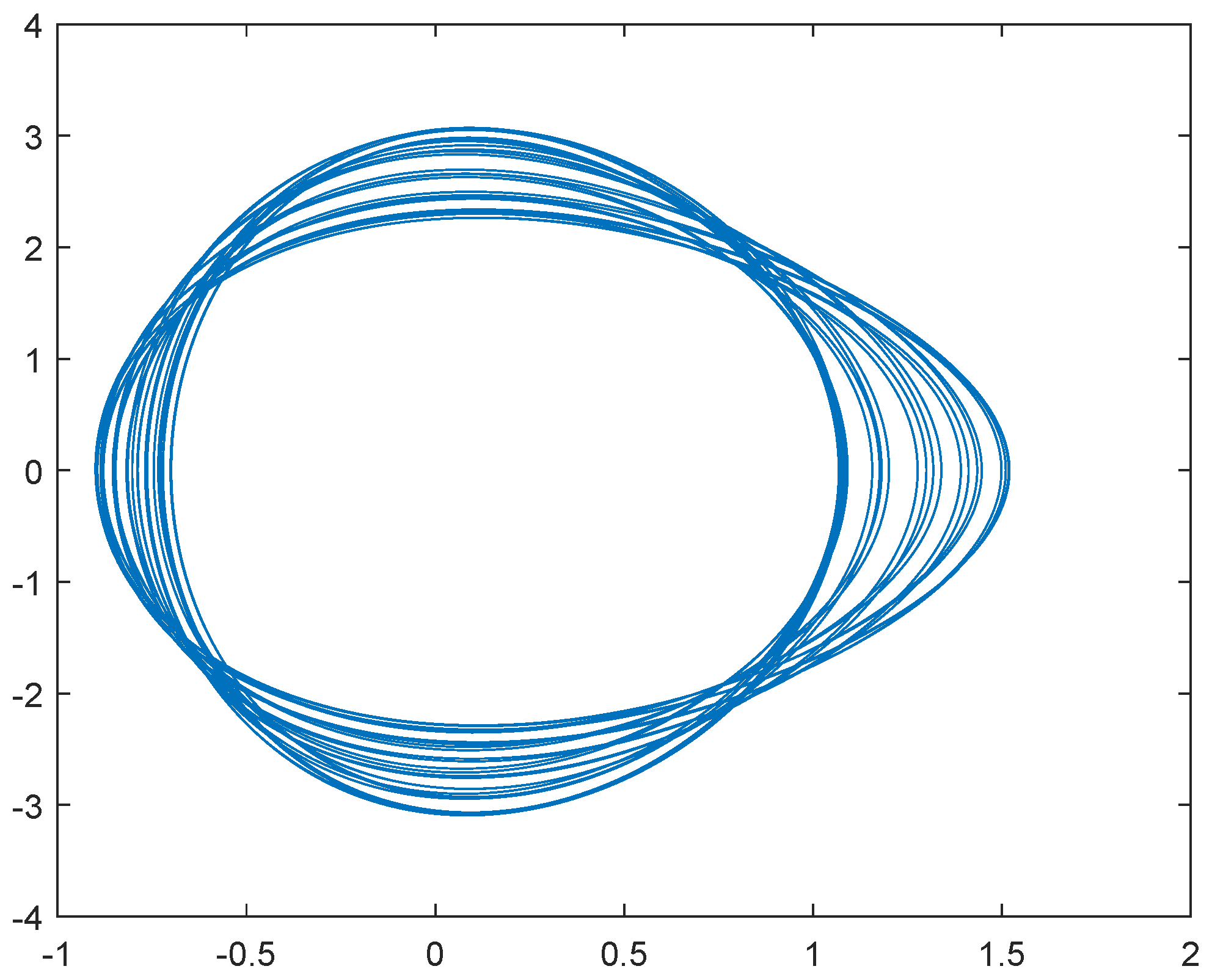
Example 3.
Consider the following ODE
where , , , , .
Obviously, and the condition holds. A simple computation gives , , , , , . Therefore, the condition also holds. By solving the following two quadratic equations
we yield that , , and . Thus,
Therefore, we conclude from Theorem 2 that (32) has at least a -periodic positive solution .
5. Conclusions
The Sturm–Liouville equation is a very famous differential equation. Many scholars have conducted extensive and in-depth research on its dynamics and have made many excellent achievements. In this manuscript, it is novel and interesting for us to establish the coincidence degree theory of Equation (1) and study the existence of its periodic solutions. We obtain some new and easily verifiable sufficient criteria for the existence of periodic solutions. Examples 1 and 2 and their simulations are applied to verify the correctness of Theorem 1 under the conditions of and , respectively. Using our method, we can estimate the existence region of periodic solutions. Our results are a useful supplement to the theory of periodic solutions of the Sturm–Liouville equation, and expand the application scope of coincidence degree theory. Based on this paper, we will further continue to study the dynamics of Equation (1) under pulse, delay and random effects. In addition, inspired by the papers [13,14,15,16,17,18,19,20,22,23,24,42,43,44,45,46,47,48,49,50,51,52], we will also study the Sturm–Liouville equation involving fractional differential as well as reaction–diffusion terms in the future.
Funding
The APC was funded by research start-up funds for high-level talents of Taizhou University.
Institutional Review Board Statement
Not applicable.
Informed Consent Statement
Not applicable.
Data Availability Statement
Not applicable.
Acknowledgments
The author would like to express his heartfelt gratitude to the editors and reviewers for their constructive comments.
Conflicts of Interest
The author declares no conflict of interest.
References
- Liu, C.; Li, B. Reconstructing a second–order Sturm–Liouville operator by an energetic boundary function iterative method. Appl. Math. Lett. 2017, 73, 49–55. [Google Scholar] [CrossRef]
- Bondarenko, N. Finite-difference approximation of the inverse Sturm–Liouville problem with frozen argument. Appl. Math. Comput. 2022, 413, 126653. [Google Scholar] [CrossRef]
- Kravchenko, V. On a method for solving the inverse Sturm–Liouville problem. J. Inverse Ill-Pose. P. 2019, 27, 401–407. [Google Scholar] [CrossRef]
- Kravchenko, V.; Torba, S. A direct method for solving inverse Sturm–Liouville problems. Inverse Probl. 2021, 37, 015015. [Google Scholar] [CrossRef]
- Kravchenko, V.; Torba, S. A practical method for recovering Sturm–Liouville problems from the Weyl function. Inverse Probl. 2021, 37, 065011. [Google Scholar] [CrossRef]
- Yang, C.; Bondarenko, N.; Xu, X. An inverse problem for the Sturm–Liouville pencil with arbitrary entire functions in the boundary condition. Inverse Probl. Imaging 2020, 14, 153–169. [Google Scholar] [CrossRef] [Green Version]
- Yang, C.; Wang, F.; Huang, Z. Ambarzumyan theorems for Dirac operators. Acta Math. Appl. Sin.-E 2021, 37, 287–298. [Google Scholar] [CrossRef]
- Sadovnichii, V.; Sultanaev, Y.; Valeev, N. Reconstruction of nonsplitting boundary conditions of the Sturm–Liouville operator from a minimal set of eigenvalues. Differ. Equ. 2020, 56, 1290–1297. [Google Scholar] [CrossRef]
- Dalvand, Z.; Hajarian, M. Solving generalized inverse eigenvalue problems via L–BFGS–B method. Inverse Probl. Sci. Eng. 2020, 28, 1719–1746. [Google Scholar] [CrossRef]
- Delgado, B.; Khmelnytskaya, K.; Kravchenko, V. The transmutation operator method for efficient solution of the inverse Sturm–Liouville problem on a half–line. Math. Method Appl. Sci. 2019, 42, 7359–7366. [Google Scholar] [CrossRef]
- Bason, G. Inverse method identification of thermophysical properties based on solotone effect analysis for discontinuous Sturm–Liouville systems. Inverse Probl. Sci. Eng. 2019, 27, 1718–1739. [Google Scholar] [CrossRef]
- Yang, C.; Bondarenko, N. Local solvability and stability of inverse problems for Sturm–Liouville operators with a discontinuity. J. Differ. Equ. 2020, 268, 6173–6188. [Google Scholar] [CrossRef] [Green Version]
- Ali, M.; Aziz, S.; Malik, S. Inverse problem for a space–time fractional diffusion equation: Application of fractional Sturm–Liouville operator. Math. Method Appl. Sci. 2018, 40, 2733–2747. [Google Scholar] [CrossRef]
- Ali, M.; Aziz, S.; Malik, S. Inverse problem for a multi–parameters space–time fractional diffusion equation with nonlocal boundary conditions: Operational calculus approach. J. Pseudo–Differ. Oper. 2022, 13, 3. [Google Scholar] [CrossRef]
- Sa’idu, A.; Koyunbakan, H. Inverse fractional Sturm–Liouville problem with eigenparameter in the boundary conditions. Math. Method Appl. Sci. 2022, in press. [Google Scholar] [CrossRef]
- Djennadi, S.; Shawagfeh, N.; Abu Arqub, O. A fractional Tikhonov regularization method for an inverse backward and source problems in the time–space fractional diffusion equations. Chaos Solitons Fract. 2021, 150, 111127. [Google Scholar] [CrossRef]
- Geng, X.; Cheng, H.; Fan, W. A note on analytical solution for the time–fractional telegraph equation by the method of separating variables. J. Math. Anal. Appl. 2022, 512, 126144. [Google Scholar] [CrossRef]
- Batiha, I.; Ouannas, A.; Albadarneh, R.; Al-Nana, A.A.; Momani, S. Existence and uniqueness of solutions for generalized Sturm–Liouville and Langevin equations via Caputo-Hadamard fractional–order operator. Eng. Comput. 2022, 39, 2581–2603. [Google Scholar] [CrossRef]
- Moutamal, M.; Joseph, C. Optimal control of fractional Sturm–Liouville wave equations on a star graph. Optimization 2022, in press. [Google Scholar] [CrossRef]
- Javed, S.; Malik, S. Some inverse problems for fractional integro–differential equation involving two arbitrary kernels. Z. Angew. Math. Phys. 2022, 73, 40. [Google Scholar] [CrossRef]
- Heydarpour, Z.; Izadi, J.; George, R.; Ghaderi, M.; Rezapour, S. On a partial fractional hybrid version of generalized Sturm–Liouville–Langevin equation. Fractal Fract. 2022, 6, 269. [Google Scholar] [CrossRef]
- Klimek, M.; Ciesielski, M.; Blaszczyk, T. Exact and numerical solution of the fractional Sturm–Liouville problem with Neumann boundary conditions. Entropy 2022, 24, 143. [Google Scholar] [CrossRef] [PubMed]
- Min, D.; Chen, F. Variational Methods to the p–Laplacian type nonlinear fractional impulsive differential equations with Sturm-Liouville boundary value problems. Fract. Calc. Appl. Anal. 2021, 24, 1069–1093. [Google Scholar] [CrossRef]
- Paknazar, M.; De La Sen, M. Fractional coupled hybrid Sturm–Liouville differential equation with multi–point boundary coupled hybrid condition. Axioms 2021, 10, 65. [Google Scholar] [CrossRef]
- Koyunbakan, H. Reconstruction of potential in discrete Sturm–Liouville problem. Qual. Theory Dyn. Syst. 2022, 21, 13. [Google Scholar] [CrossRef]
- Allahverdiev, B.; Tuna, H. Conformable fractional Sturm–Liouville problems on time scales. Math. Method Appl. Sci. 2022, 45, 2299–2314. [Google Scholar] [CrossRef]
- Kuznetsova, M. On recovering the Sturm–Liouville differential operators on time scales. Math. Notes 2021, 109, 74–88. [Google Scholar] [CrossRef]
- Adalar, I.; Ozkan, A. An interior inverse Sturm–Liouville problem on a time scale. Anal. Math. Phys. 2020, 10, 58. [Google Scholar] [CrossRef]
- Heidarkhani, S.; Moradi, S.; Caristi, G. Existence results for a dynamic Sturm–Liouville boundary value problem on time scales. Optim. Lett. 2020, 15, 2497–2514. [Google Scholar] [CrossRef]
- Kuznetsova, M. A uniqueness theorem on inverse spectral problems for the Sturm–Liouville differential operators on time scales. Results Math. 2020, 75, 44. [Google Scholar] [CrossRef]
- Ozkan, A.; Adalar, I. Half–inverse Sturm-Liouville problem on a time scale. Inverse Probl. 2020, 36, 025015. [Google Scholar] [CrossRef]
- Ao, J.; Wang, J. Eigenvalues of Sturm–Liouville problems with distribution potentials on time scales. Quaest. Math. 2019, 42, 1185–1197. [Google Scholar] [CrossRef]
- Ao, J.; Wang, J. Finite spectrum of Sturm–Liouville problems with eigenparameter–dependent boundary conditions on time scales. Filomat 2019, 33, 1747–1757. [Google Scholar] [CrossRef] [Green Version]
- Barilla, D.; Bohner, M.; Heidarkhani, S.; Moradi, S. Existence results for dynamic Sturm–Liouville boundary value problems via variational methods. Appl. Math. Comput. 2021, 409, 125614. [Google Scholar] [CrossRef]
- Ishkin, K.; Davletova, L. Regularized trace of a Sturm–Liouville operator on a curve with a regular singularity on the chord. Differ. Equ. 2020, 56, 1257–1269. [Google Scholar] [CrossRef]
- Hu, X.; Liu, L.; Wu, L.; Zhu, H. Singularity of the n–th eigenvalue of high dimensional Sturm–Liouville problems. J. Differ. Equ. 2019, 266, 4106–4136. [Google Scholar] [CrossRef] [Green Version]
- Bondarenko, N. Inverse problems for the matrix Sturm–Liouville equation with a Bessel–type singularity. Appl. Anal. 2018, 97, 1209–1222. [Google Scholar] [CrossRef]
- Chen, L. A sub–density theorem of Sturm–Liouville eigenvalue problem with finitely many singularities. J. Contemp. Math. Anal. 2018, 53, 1–5. [Google Scholar] [CrossRef]
- Gaines, R.; Mawhin, J. Coincidence Degree and Nonlinear Differetial Equitions; Lecture Notes in Mathematics Series; Springer: Berlin/Heidelberg, Germany, 1977; Volume 568. [Google Scholar]
- Zhao, K. Local exponential stability of four almost–periodic positive solutions for a classic Ayala–Gilpin competitive ecosystem provided with varying–lags and control terms. Int. J. Control 2022, in press. [Google Scholar] [CrossRef]
- Zhao, K. Local exponential stability of several almost periodic positive solutions for a classical controlled GA–predation ecosystem possessed distributed delays. Appl. Math. Comput. 2023, 437, 127540. [Google Scholar] [CrossRef]
- Zhang, T.; Li, Y. Exponential Euler scheme of multi–delay Caputo–Fabrizio fractional–order differential equations. Appl. Math. Lett. 2022, 124, 107709. [Google Scholar] [CrossRef]
- Zhang, T.; Xiong, L. Periodic motion for impulsive fractional functional differential equations with piecewise Caputo derivative. Appl. Math. Lett. 2020, 101, 106072. [Google Scholar] [CrossRef]
- Zhang, T.; Li, Y. Global exponential stability of discrete–time almost automorphic Caputo–Fabrizio BAM fuzzy neural networks via exponential Euler technique. Knowl.–Based Syst. 2022, 246, 108675. [Google Scholar] [CrossRef]
- Zhang, T.; Zhou, J.; Liao, Y. Exponentially stable periodic oscillation and Mittag–Leffler stabilization for fractional-order impulsive control neural networks with piecewise Caputo derivatives. IEEE Trans. Cybern. 2022, 52, 9670–9683. [Google Scholar] [CrossRef] [PubMed]
- Zhao, K. Stability of a nonlinear fractional Langevin system with nonsingular exponential kernel and delay control. Discret. Dyn. Nat. Soc. 2022, 2022, 9169185. [Google Scholar] [CrossRef]
- Zhao, K. Existence, stability and simulation of a class of nonlinear fractional Langevin equations involving nonsingular Mittag–Leffler kernel. Fractal Fract. 2022, 6, 469. [Google Scholar] [CrossRef]
- Zhao, K. Stability of a nonlinear ML–nonsingular kernel fractional Langevin system with distributed lags and integral control. Axioms 2022, 11, 350. [Google Scholar] [CrossRef]
- Huang, H.; Zhao, K.; Liu, X. On solvability of BVP for a coupled Hadamard fractional systems involving fractional derivative impulses. AIMS Math. 2022, 7, 19221–19236. [Google Scholar] [CrossRef]
- Zhao, K. Stability of a nonlinear Langevin system of ML–type fractional derivative affected by time–varying delays and differential feedback control. Fractal Fract. 2022, 6, 725. [Google Scholar] [CrossRef]
- Zhao, K. Global stability of a novel nonlinear diffusion online game addiction model with unsustainable control. AIMS Math. 2022, 7, 20752–20766. [Google Scholar] [CrossRef]
- Zhao, K. Probing the oscillatory behavior of internet game addiction via diffusion PDE model. Axioms 2022, 11, 649. [Google Scholar] [CrossRef]
Figure 1.
Phase portrait of (30) with .
Figure 1.
Phase portrait of (30) with .

Figure 2.
Phase portrait of (31) with .
Figure 2.
Phase portrait of (31) with .

Figure 3.
Phase portrait of (32) with .
Figure 3.
Phase portrait of (32) with .

Disclaimer/Publisher’s Note: The statements, opinions and data contained in all publications are solely those of the individual author(s) and contributor(s) and not of MDPI and/or the editor(s). MDPI and/or the editor(s) disclaim responsibility for any injury to people or property resulting from any ideas, methods, instructions or products referred to in the content. |
© 2022 by the author. Licensee MDPI, Basel, Switzerland. This article is an open access article distributed under the terms and conditions of the Creative Commons Attribution (CC BY) license (https://creativecommons.org/licenses/by/4.0/).
Share and Cite
MDPI and ACS Style
Zhao, K. Coincidence Theory of a Nonlinear Periodic Sturm–Liouville System and Its Applications. Axioms 2022, 11, 726. https://doi.org/10.3390/axioms11120726
AMA Style
Zhao K. Coincidence Theory of a Nonlinear Periodic Sturm–Liouville System and Its Applications. Axioms. 2022; 11(12):726. https://doi.org/10.3390/axioms11120726
Chicago/Turabian StyleZhao, Kaihong. 2022. "Coincidence Theory of a Nonlinear Periodic Sturm–Liouville System and Its Applications" Axioms 11, no. 12: 726. https://doi.org/10.3390/axioms11120726
Note that from the first issue of 2016, this journal uses article numbers instead of page numbers. See further details here.