Probing the Oscillatory Behavior of Internet Game Addiction via Diffusion PDE Model

Abstract

We establish a non-linear diffusion partial differential equation (PDE) model to depict the dynamic mechanism of Internet gaming disorder (IGD). By constructing appropriate super- and sub-solutions and applying Schauder’s fixed point theorem and continuation method, we study the existence and asymptotic stability of traveling wave solutions to probe into the oscillating behavior of IGD. An example is numerically simulated to examine the correctness of our outcomes.

1. Introduction

1.1. Background and Model

In the past decade, with the continuous popularization of the Internet, the number of Internet users has increased sharply. The convenience and other benefits of the Internet are obvious to all. However, there is also some harmful content on the Internet, such as pornography, violence, online games and so on. In particular, various types of Internet games are full of major Internet websites with legal identities. These Internet games have attracted a large number of game players, especially teenagers. Many game players become addicted to Internet games. People with Internet gaming addiction tend to be impulsive, violent, misanthropic and withdrawn. This not only brings great harm to the physical and mental health of Internet game addicts but also endangers society and their families. In recent years, the number of Internet game addicts has continued to rise. This phenomenon has been widely concerning and studied. The World Health Organization [1] has pointed out that Internet game addiction is a new disease. The disease is named Internet gaming disorder (IGD) and is characterized by “Persistent and recurrent use of the Internet to engage in games, often with other players, leading to clinically significant impairment or distress” [2]. IGD is often referred to as a mental illness. The Diagnostic and Statistical Manual of Mental Disorders [3,4] provides some classifications of IGD. In order to cure and reduce the number of people with IGD, scholars from all walks of life have begun to study IGD from various aspects. Some researchers [5,6,7,8,9] use mathematical theories and methods to study IGD by establishing mathematical models.

In this context, we also try to use calculus methods to establish a differential equation model to study IGD. To this end, we make the underlying assumptions as follows:

(i)

Internet game players are simply divided into two categories: moderate gamers M and addictive gamers A;

(ii)

Because it is very difficult to stop playing games through self-control, Internet game players M and A are treated.

(iii)

The spatial distribution of the number of Internet game players is very uneven, which is concentrated in places such as Internet cafes and schools, and then gradually decreases outward. Based on this, we assume that the population distribution of the two types of Internet game players is diffuse in space.

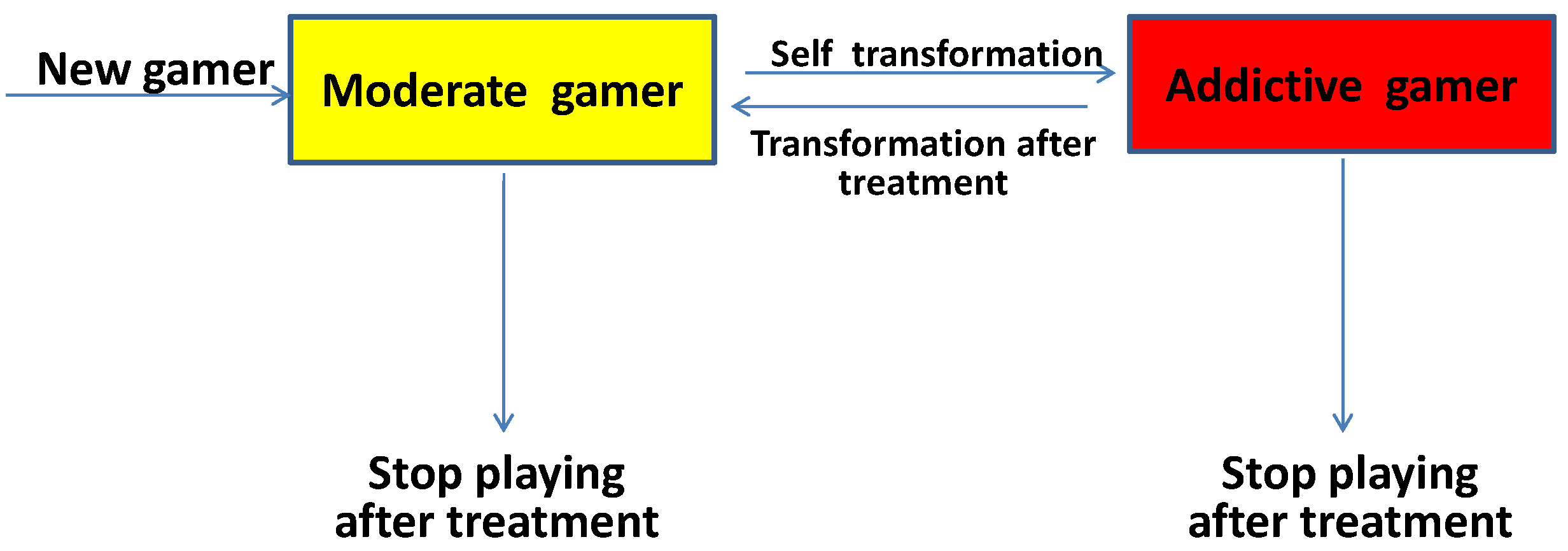
Below, we give the state changes in Internet game players, as shown in the Figure 1.

Based on the assumptions $\left(\mathrm{i}\right)$–$\left(\mathrm{iii}\right)$, we explain the process described in Figure 1 in detail. $M(x,t)$ and $A(x,t)$ stand for the population density of moderate gamers and addictive gamers at time t and position x, respectively. In time period $\Delta t$, the moderate gamers M have increased by $\alpha M(x,t)\Delta t$ and $\delta A(x,t)\Delta t$ because some non-gamers have become new gamers and some addictive gamers have converted to moderate gamers after treatment. In the meantime, the moderate gamers M have declined by $\beta M(x,t)A(x,t)\Delta t$ and ${\gamma }_{1}M(x,t)\Delta t$ because some moderate gamers have become addictive gamers and another moderate gamers have converted to non-gamers after treatment. Vice versa, the addictive gamers A have only raised by $\beta M(x,t)A(x,t)\Delta t$ because of the transformation from moderate gamers to addictive gamers. At the same time, the addictive gamers M have reduced by $\delta A(x,t)\Delta t$ and ${\gamma }_{2}A(x,t)\Delta t$ because some addictive gamers have become moderate gamers and another addictive gamers have converted to non-gamers after treatment. Furthermore, we added the diffusion terms $d_1\frac{{\partial }^{2}M}{\partial x^2}\Delta t$ and $d_2\frac{{\partial }^{2}A}{\partial x^2}\Delta t$, where $d_1$ and $d_2$ are the diffusion coefficients. Through the above analysis, we build a new model as follows:

$$\begin{array}{c}\hfill \left\{\begin{array}{c}\frac{\partial M}{\partial t}=d_1\frac{{\partial }^2}{\partial x^2}M(x,t)+\alpha -\beta M(x,t)A(x,t)-{\gamma }_{1}M(x,t)+\delta A(x,t),\hfill \\ \frac{\partial A}{\partial t}=d_2\frac{{\partial }^2}{\partial x^2}A(x,t)+\beta M(x,t)A(x,t)-({\gamma }_2+\delta )A(x,t),\hfill \end{array}\right.\end{array}$$

(1)

where $(x,t)\in \mathbb{R}\times (0,\infty )$, $\alpha ,\beta ,\delta ,{\gamma }_1,{\gamma }_2,d_1,d_2>0$ are some constants.

Remark 1.

In (1), if there is lack of treatment and diffusion, then $M+A=M\left(0\right)+A\left(0\right)+\alpha t\to +\infty$, as $t\to +\infty$. This will lead to everyone eventually becoming a gamer. Therefore, proper treatment is necessary. Moreover, there are two kinds of healing effects on addicted gamers. One is to cure them completely and make them non-gamers. The other is to reduce their addiction and make them moderate gamers. This shows that game addiction is a stubborn psychological disease. It is difficult to eradicate completely.

1.2. Significance and Contribution

The traveling wave solutions of non-linear reaction–diffusion equations have important applications in many disciplines, such as biological dynamics [10,11], epidemic dynamics [12,13,14] and tumor dynamics [15,16]. Therefore, the study of traveling wave solutions and their properties of diffusion of non-linear partial differential equation models has attracted the attention of many scholars. There have been many good works [17,18,19,20,21,22,23] dealing with the traveling wave of reaction–diffusion equations. Enlightened by the ideas and methods in these references, this paper focuses on the existence of traveling wave solutions to Equation (1). So, let $M(x,t)=\tilde{M}\left(\xi \right)$, $A(x,t)=\tilde{A}\left(\xi \right)$, $\xi =x+ct (c>0)$, then (1) becomes

$$\begin{array}{c}\hfill \left\{\begin{array}{c}c{\tilde{M}}^{\prime }\left(\xi \right)-d_1{\tilde{M}}^{″}\left(\xi \right)=\alpha -\beta \tilde{M}\left(\xi \right)\tilde{A}\left(\xi \right)-{\gamma }_1\tilde{M}\left(\xi \right)+\delta \tilde{A}\left(\xi \right),\hfill \\ c{\tilde{A}}^{\prime }\left(\xi \right)-d_2{\tilde{A}}^{″}\left(\xi \right)=\beta \tilde{M}\left(\xi \right)\tilde{A}\left(\xi \right)-({\gamma }_2+\delta )\tilde{A}\left(\xi \right).\hfill \end{array}\right.\end{array}$$

(2)

It is easy to verify that Equation (2) has a unique non-negative constant solution $(\tilde{M}\left(\xi \right),\tilde{A}\left(\xi \right))$$=(\frac{\alpha }{{\gamma }_1},0)$. Let $\mathcal{M}\left(\xi \right)=\tilde{M}\left(\xi \right)-\frac{\alpha }{{\gamma }_1}$, $\mathcal{A}\left(\xi \right)=\tilde{A}\left(\xi \right)$, then Equation (2) changes into

$$\begin{array}{c}\hfill \left\{\begin{array}{c}c{\mathcal{M}}^{\prime }\left(\xi \right)-d_1{\mathcal{M}}^{″}\left(\xi \right)=-\beta \mathcal{M}\left(\xi \right)\mathcal{A}\left(\xi \right)-{\gamma }_1\mathcal{M}\left(\xi \right)-(\alpha \beta {\gamma }_1^{-1}-\delta )\mathcal{A}\left(\xi \right),\hfill \\ c{\mathcal{A}}^{\prime }\left(\xi \right)-d_2{\mathcal{A}}^{″}\left(\xi \right)=\beta \mathcal{M}\left(\xi \right)\mathcal{A}\left(\xi \right)+(\alpha \beta {\gamma }_1^{-1}-{\gamma }_2-\delta )\mathcal{A}\left(\xi \right).\hfill \end{array}\right.\end{array}$$

(3)

The whole paper requires the following assumptions.

$\left(\mathrm{A}\right)$

For some given constants $\alpha ,\beta ,\delta ,{\gamma }_1,{\gamma }_2,d_1,d_2>0$ and an unknown constant $c>0$, there are ${\gamma }_2+\delta <\alpha \beta {\gamma }_1^{-1}$ and $c>2\sqrt{d_2(\alpha \beta {\gamma }_1^{-1}-{\gamma }_2-\delta )}$.

The paper mainly includes the following contributions. $\left(\mathrm{a}\right)$ We propose a novel diffusion PDE (1) modeling Internet game addiction, which is rare in previous papers. $\left(\mathrm{b}\right)$ Based on Schauder’s fixed point theorem and continuation method, we study the existence and asymptotic stability of traveling waves of the model (1) to reveal the oscillating behavior of IGD. $\left(\mathrm{c}\right)$ Our research provides some theoretical help for the study and treatment of IGD. The remaining structure of the paper is as follows. Section 2 introduces super- and sub-solutions and their properties. Section 3 gives the detailed proof process of the existence of traveling waves. Section 4 studies the global asymptotic stability of traveling waves. In Section 5, we provide an example and carry out numerical simulation to examine the validity of our results. Section 6 is a brief summary.

2. Super- and Sub-Solutions

This section provides the upper and lower solutions of (3) and their properties. Define the super-solutions $\overline{P}\left(\xi \right)=e^{\lambda \xi }$, and $\overline{Q}\left(\xi \right)=e^{\mu \xi }$, where

$$\begin{array}{c}\hfill \lambda =\frac{c+\sqrt{c^2+4d_1{\gamma }_1}}{2d_1},\mu =\frac{c+\sqrt{c^2-4d_2(\alpha \beta {\gamma }_1^{-1}-{\gamma }_2-\delta )}}{2d_2}.\end{array}$$

By the condition $\left(\mathrm{B}\right)$, one has $\lambda ,\mu >0$, and

$$\begin{array}{c}\hfill c{\overline{P}}^{\prime }\left(\xi \right)-d_1{\overline{P}}^{″}\left(\xi \right)=-{\gamma }_1\overline{P}\left(\xi \right),c{\overline{Q}}^{\prime }\left(\xi \right)-d_2{\overline{Q}}^{″}\left(\xi \right)=(\alpha \beta {\gamma }_1^{-1}-{\gamma }_2-\delta )\overline{Q}\left(\xi \right).\end{array}$$

Take the sub-solutions $\underline{P}\left(\xi \right)=e^{\lambda \xi }-\mathcal{P}{e}^{(\lambda -ϵ)\xi }$ and $\underline{Q}\left(\xi \right)=e^{\mu \xi }-\mathcal{Q}{e}^{(\mu -ϵ)\xi }$, where $\mathcal{P},\mathcal{Q}>1$ and $ϵ\in (0,min\{\lambda ,\mu \left\}\right)$ are small enough such that

$$\rho =-d_1{(\lambda -ϵ)}^2+c(\lambda -ϵ)>0,\varrho =-d_2{(\mu -ϵ)}^2+c(\mu -ϵ)-(\alpha \beta {\gamma }_1^{-1}-{\gamma }_2-\delta )>0,$$

$$\underline{\xi }\triangleq max\left\{\frac{ln\mathcal{P}}{ϵ},\frac{ln\mathcal{Q}}{ϵ}\right\}<min\left\{\frac{1}{\lambda }ln\frac{\rho (\alpha \beta {\gamma }_1^{-1}-\delta )}{\beta {\gamma }_1},\frac{1}{\mu }ln\frac{\mathcal{P}{\gamma }_1}{\alpha \beta {\gamma }_1^{-1}-\delta }\right\}\triangleq \overline{\xi }.$$

When $\underline{\xi }<\xi <\overline{\xi }$, we obtain $\underline{P}\left(\xi \right),\underline{Q}\left(\xi \right)>0$, and

$$\begin{array}{cc}\hfill & c{\underline{P}}^{\prime }\left(\xi \right)-d_1{\underline{P}}^{″}\left(\xi \right)+\beta \underline{P}\left(\xi \right)\underline{Q}\left(\xi \right)+{\gamma }_1\underline{P}\left(\xi \right)+(\alpha \beta {\gamma }_1^{-1}-\delta )\underline{Q}\left(\xi \right)\hfill \\ \hfill =& c\left[\lambda e^{\lambda \xi }-\mathcal{P}(\lambda -ϵ)e^{(\lambda -ϵ)\xi }\right]-d_1\left[{\lambda }^2{e}^{\lambda \xi }-\mathcal{P}{(\lambda -ϵ)}^2{e}^{(\lambda -ϵ)\xi }\right]+{\gamma }_1\left[e^{\lambda \xi }-\mathcal{P}{e}^{(\lambda -ϵ)\xi }\right]\hfill \\ \hfill & +\beta \left[e^{\lambda \xi }-\mathcal{P}{e}^{(\lambda -ϵ)\xi }\right]\left[e^{\mu \xi }-\mathcal{Q}{e}^{(\mu -ϵ)\xi }\right]+\left(\alpha \beta {\gamma }_1^{-1}-\delta \right)\left[e^{\mu \xi }-b{e}^{(\mu -ϵ)\xi }\right]\hfill \\ \hfill <& \left[\mathcal{P}{d}_1{(\lambda -ϵ)}^2-\mathcal{P}c(\lambda -ϵ)-\mathcal{P}{\gamma }_1\right]e^{(\lambda -ϵ)\xi }+\beta e^{\lambda \xi }{e}^{\mu \xi }+\left(\alpha \beta {\gamma }_1^{-1}-\delta \right)e^{\mu \xi }\hfill \\ \hfill <& -\left[\mathcal{P}\rho -\beta e^{\lambda \xi }{e}^{\mu \xi }+\mathcal{P}{\gamma }_1-\left(\alpha \beta {\gamma }_1^{-1}-\delta \right)e^{\mu \xi }\right]e^{(\lambda -ϵ)\xi }\hfill \\ \hfill <& -\left[\mathcal{P}\rho -\beta ·\frac{\rho (\alpha \beta {\gamma }_1^{-1}-\delta )}{\beta {\gamma }_1}·\frac{\mathcal{P}{\gamma }_1}{\alpha \beta {\gamma }_1^{-1}-\delta }+\mathcal{P}{\gamma }_1-\left(\alpha \beta {\gamma }_1^{-1}-\delta \right)·\frac{\mathcal{P}{\gamma }_1}{\alpha \beta {\gamma }_1^{-1}-\delta }\right]e^{(\lambda -ϵ)\xi }=0,\hfill \end{array}$$

$$\begin{array}{cc}\hfill & c{\underline{Q}}^{\prime }\left(\xi \right)-d_2{\underline{Q}}^{″}\left(\xi \right)-\beta \underline{P}\left(\xi \right)\underline{Q}\left(\xi \right)-(\alpha \beta {\gamma }_1^{-1}-{\gamma }_2-\delta )\underline{Q}\left(\xi \right)\hfill \\ \hfill =& c\left[\mu e^{\mu \xi }-\mathcal{Q}(\mu -ϵ)e^{(\mu -ϵ)\xi }\right]-d_2\left[{\mu }^2{e}^{\mu \xi }-\mathcal{Q}{(\mu -ϵ)}^2{e}^{(\mu -ϵ)\xi }\right]\hfill \\ \hfill & -\beta \left[e^{\lambda \xi }-\mathcal{P}{e}^{(\lambda -ϵ)\xi }\right]\left[e^{\mu \xi }-\mathcal{Q}{e}^{(\mu -ϵ)\xi }\right]-(\alpha \beta {\gamma }_1^{-1}-{\gamma }_2-\delta )\left[e^{\mu \xi }-\mathcal{Q}{e}^{(\mu -ϵ)\xi }\right]\hfill \\ \hfill <& -\mathcal{Q}\left[-d_2{(\mu -ϵ)}^2+c(\mu -ϵ)-(\alpha \beta {\gamma }_1^{-1}-{\gamma }_2-\delta )\right]e^{(\mu -ϵ)\xi }=-\mathcal{Q}\varrho e^{(\mu -ϵ)\xi }<0.\hfill \end{array}$$

Let $\tilde{P}\left(\xi \right)=max\{0,\underline{P}\left(\xi \right)\}$, $\tilde{Q}\left(\xi \right)=max\{0,\underline{Q}\left(\xi \right)\}$, $\xi \in \mathbb{R}$, then, we have

$$c{\tilde{P}}^{\prime }\left(\xi \right)-d_1{\tilde{P}}^{″}\left(\xi \right)+\beta \tilde{P}\left(\xi \right)\tilde{Q}\left(\xi \right)+{\gamma }_1\tilde{P}\left(\xi \right)+(\alpha \beta {\gamma }_1^{-1}-\delta )\tilde{Q}\left(\xi \right)\le 0,\forall \xi \ne \frac{ln\mathcal{P}}{ϵ},$$

$$c{\tilde{Q}}^{\prime }\left(\xi \right)-d_2{\tilde{Q}}^{″}\left(\xi \right)-\beta \tilde{P}\left(\xi \right)\tilde{Q}\left(\xi \right)-(\alpha \beta {\gamma }_1^{-1}-{\gamma }_2-\delta )\tilde{Q}\left(\xi \right)\le 0,\forall \xi \ne \frac{ln\mathcal{Q}}{ϵ}.$$

3. Existence of Traveling Wave

This section mainly discusses the existence and non-existence of traveling waves and some properties of traveling waves. We boil them down to the following theorem.

Theorem 1.

Assume that $\left(\mathrm{A}\right)$ holds, then the following assertions are true:

$\left(\mathrm{a}\right)$

For any $c>c^{*}=2\sqrt{d_2(\alpha \beta {\gamma }_1^{-1}-{\gamma }_2-\delta )}$, there is a traveling wave solution $({\tilde{M}}^{*}\left(\xi \right),$${\tilde{A}}^{*}\left(\xi \right))$ of model (1) satisfying $\underset{\xi \to -\infty }{lim}{\tilde{M}}^{*}\left(\xi \right)=\frac{\alpha }{{\gamma }_1}$, $\underset{\xi \to -\infty }{lim}{\tilde{A}}^{*}\left(\xi \right)=0$.

$\left(\mathrm{b}\right)$

$\exists {\xi }_0>0$, when $\xi \in (-\infty ,-{\xi }_0)$, ${\tilde{M}}^{*}\left(\xi \right)$ and ${\tilde{A}}^{*}\left(\xi \right)$ are monotone increasing functions.

$\left(\mathrm{c}\right)$

There is no traveling wave solution of model (1) provided that $c<c^{*}$.

$\left(\mathrm{d}\right)$

$\underset{\xi \to +\infty }{lim\; inf}{\tilde{M}}^{*}\left(\xi \right)>\frac{\alpha }{{\gamma }_1}$, $\underset{\xi \to +\infty }{lim\; inf}{\tilde{A}}^{*}\left(\xi \right)>0$.

Proof. 

(1) The proof of assertion $\left(\mathrm{a}\right)$. Here, we prove it in two steps.

Step 1: Local existence of traveling wave. For $c>2\sqrt{d_2(\alpha \beta {\gamma }_1^{-1}-{\gamma }_2-\delta )}$, consider a two-point BVP in $(-l,l)$ of the form

$$\begin{array}{c}\hfill \left\{\begin{array}{c}c{\mathcal{M}}^{\prime }\left(\xi \right)-d_1{\mathcal{M}}^{″}\left(\xi \right)=-\beta \overline{\mathcal{M}}\left(\xi \right)\overline{\mathcal{A}}\left(\xi \right)-{\gamma }_1\overline{\mathcal{M}}\left(\xi \right)-(\alpha \beta {\gamma }_1^{-1}-\delta )\overline{\mathcal{A}}\left(\xi \right)\hfill \\ \triangleq F(\overline{\mathcal{M}}\left(\xi \right),\overline{\mathcal{A}}\left(\xi \right)),\hfill \\ c{\mathcal{A}}^{\prime }\left(\xi \right)-d_2{\mathcal{A}}^{″}\left(\xi \right)=\beta \overline{\mathcal{M}}\left(\xi \right)\overline{\mathcal{M}}\left(\xi \right)+(\alpha \beta {\gamma }_1^{-1}-{\gamma }_2-\delta )\overline{\mathcal{A}}\left(\xi \right)\triangleq G(\overline{\mathcal{M}}\left(\xi \right),\overline{\mathcal{A}}\left(\xi \right)),\hfill \\ \mathcal{M}(\pm l)=\tilde{P}(\pm l),\mathcal{A}(\pm l)=\tilde{Q}(\pm l),{\mathcal{M}}^{\prime }(\pm l)={\tilde{P}}^{\prime }(\pm l),{\mathcal{A}}^{\prime }(\pm l)={\tilde{Q}}^{\prime }(\pm l),\hfill \end{array}\right.\end{array}$$

(4)

where $l>\underline{\xi }$, and

$$\begin{array}{c}\hfill \overline{\mathcal{M}}\left(\xi \right)=\left\{\begin{array}{cc}\mathcal{M}(-l),\hfill & \xi <-l,\hfill \\ \mathcal{M}\left(\xi \right),\hfill & -l\le \xi \le l,\hfill \\ \mathcal{M}\left(l\right),\hfill & \xi >l,\hfill \end{array}\right.\overline{\mathcal{A}}\left(\xi \right)=\left\{\begin{array}{cc}\mathcal{A}(-l),\hfill & \xi <-l,\hfill \\ \mathcal{A}\left(\xi \right),\hfill & -l\le \xi \le l,\hfill \\ \mathcal{A}\left(l\right),\hfill & \xi >l.\hfill \end{array}\right.\end{array}$$

(5)

By Section 2, for a solution $\left(\mathcal{M}\right(\xi ),\mathcal{A}(\xi \left)\right)$ of (4), one has $\tilde{P}\left(\xi \right)\le \mathcal{M}\left(\xi \right)\le \overline{P}\left(\xi \right)$, $\tilde{Q}\left(\xi \right)\le \mathcal{A}\left(\xi \right)\le \overline{Q}\left(\xi \right)$. Introducing a norm

$$\parallel (u,v)\parallel =max\left\{\underset{\xi \in [-l,l]}{sup}\left|u\left(\xi \right)\right|,\underset{\xi \in [-l,l]}{sup}\left|v\left(\xi \right)\right|,\underset{\xi \in [-l,l]}{sup}|u^{\prime }\left(\xi \right)|,\underset{\xi \in [-l,l]}{sup}\left|v^{\prime }\left(\xi \right)\right|\right\},$$

for $(u,v)\in C^2([-l,l],{\mathbb{R}}^2)$, then $C^2([-l,l],{\mathbb{R}}^2)$ is a Banach space. Let $\parallel (\tilde{P},\tilde{Q})\parallel =R_1$, $\parallel (\overline{P},\overline{Q})\parallel =R_2$, $R_3=R_1+R_1{d}_1{c}^{-1}\left(e^{\frac{2cl}{d_1}}-1\right)+d_1{R}_2{c}^{-2}(\beta R_2+{\gamma }_1+\alpha \beta {\gamma }_1^{-1}-\delta )\left(e^{\frac{cl}{d_1}}-1\right)\left(e^{\frac{cl}{d_1}}-e^{-\frac{cl}{d_1}}\right)$, $R_4=R_1+R_1{d}_1{c}^{-1}\left(e^{\frac{2cl}{d_2}}-1\right)+d_2{R}_2{c}^{-2}(\beta R_2+\alpha \beta {\gamma }_1^{-1}-{\gamma }_2-\delta )\left(e^{\frac{cl}{d_2}}-1\right)\left(e^{\frac{cl}{d_2}}-e^{-\frac{cl}{d_2}}\right)$, $R=max\{R_1,R_2,R_3,R_4\}$, $\Omega =\{(u,v)\in C^2([-l,l],{\mathbb{R}}^2):\parallel (u,v)\parallel <R+1\}$. For $(u,v)\in \Omega$, define a mapping $\mathcal{L}={({\mathcal{L}}_1,{\mathcal{L}}_2)}^T:\Omega \to {\mathbb{R}}^2$ as

$$\begin{array}{c}\hfill \left(\mathcal{L}(u,v)\right)\left(\xi \right)=\left(\begin{array}{c}\left(\mathcal{L}\right(u,v\left)\right)\left(\xi \right)\\ \left(\mathcal{L}\right(u,v\left)\right)\left(\xi \right)\end{array}\right),\end{array}$$

(6)

where

$$\left({\mathcal{L}}_1(u,v)\right)\left(\xi \right)=u(-l)+u^{\prime }(-l)e^{\frac{cl}{d_1}}{\int }_{-l}^{\xi }{e}^{\frac{c}{d_1}\tau }d\tau -\frac{1}{d_1}{\int }_{-l}^{\xi }\left[{\int }_{-l}^{\tau }{e}^{-\frac{c}{d_1}(s-\tau )}F(\overline{u}\left(s\right),\overline{v}\left(s\right))ds\right]d\tau ,$$

$$\left({\mathcal{L}}_2(u,v)\right)\left(\xi \right)=v(-l)+v^{\prime }(-l)e^{\frac{cl}{d_2}}{\int }_{-l}^{\xi }{e}^{\frac{c}{d_2}\tau }d\tau -\frac{1}{d_2}{\int }_{-l}^{\xi }\left[{\int }_{-l}^{\tau }{e}^{-\frac{c}{d_2}(s-\tau )}G(\overline{u}\left(s\right),\overline{v}\left(s\right))ds\right]d\tau .$$

By the boundary conditions, $\left(\mathrm{A}\right)$ and (6), we have

$$\begin{array}{cc}\hfill & \left|\right({\mathcal{L}}_1(u,v)\left)\left(\xi \right)\right|\hfill \\ \hfill =& |\tilde{P}(-l)+{\tilde{P}}^{\prime }(-l)e^{\frac{cl}{d_1}}{\int }_{-l}^{\xi }{e}^{\frac{c}{d_1}\tau }d\tau -\frac{1}{d_1}{\int }_{-l}^{\xi }\left[{\int }_{-l}^{\tau }{e}^{-\frac{c}{d_1}(s-\tau )}F(\overline{u}\left(s\right),\overline{v}\left(s\right))ds\right]d\tau |\hfill \\ \hfill \le & |\tilde{P}(-l)|+|{\tilde{P}}^{\prime }(-l)|e^{\frac{cl}{d_1}}{\int }_{-l}^l{e}^{\frac{c}{d_1}\tau }d\tau +\frac{1}{d_1}{\int }_{-l}^l\left[{\int }_{-l}^{\tau }{e}^{-\frac{c}{d_1}(s-\tau )}\left|F(\overline{u}\left(s\right),\overline{v}\left(s\right))\right|ds\right]d\tau \hfill \\ \hfill \le & R_1+R_1\frac{d_1}{c}\left(e^{\frac{2cl}{d_1}}-1\right)+\frac{1}{d_1}{\int }_{-l}^l[{\int }_{-l}^l{e}^{-\frac{c}{d_1}(s-\tau )}\left[\beta \right|\overline{u}\left(s\right)\left|\right|\overline{v}\left(s\right)\left)\right|\hfill \\ \hfill & +{\gamma }_1|\overline{u}\left(s\right)|+(\alpha \beta {\gamma }_1^{-1}-\delta )|\overline{v}\left(s\right)\left|\right]ds]d\tau \hfill \\ \hfill \le & R_1+R_1{d}_1{c}^{-1}\left(e^{\frac{2cl}{d_1}}-1\right)+d_1{R}_2{c}^{-2}(\beta R_2+{\gamma }_1+\alpha \beta {\gamma }_1^{-1}-\delta )\left(e^{\frac{cl}{d_1}}-1\right)\left(e^{\frac{cl}{d_1}}-e^{-\frac{cl}{d_1}}\right)\hfill \\ \hfill =& R_3<R+1.\hfill \end{array}$$

(7)

Similar to (7), we obtain

$$\begin{array}{cc}\hfill & \left|\right({\mathcal{L}}_2(u,v)\left)\left(\xi \right)\right|\hfill \\ \hfill =& |v(-l)+v^{\prime }(-l)e^{\frac{cl}{d_2}}{\int }_{-l}^{\xi }{e}^{\frac{c}{d_2}\tau }d\tau -\frac{1}{d_2}{\int }_{-l}^{\xi }\left[{\int }_{-l}^{\tau }{e}^{-\frac{c}{d_2}(s-\tau )}G(\overline{u}\left(s\right),\overline{v}\left(s\right))ds\right]d\tau |\hfill \\ \hfill \le & R_1+R_1{d}_1{c}^{-1}\left(e^{\frac{2cl}{d_2}}-1\right)+d_2{R}_2{c}^{-2}(\beta R_2+\alpha \beta {\gamma }_1^{-1}-{\gamma }_2-\delta )\left(e^{\frac{cl}{d_2}}-1\right)\left(e^{\frac{cl}{d_2}}-e^{-\frac{cl}{d_2}}\right)\hfill \\ \hfill =& R_4<R+1.\hfill \end{array}$$

(8)

From (7) and (8), one knows that $\mathcal{L}(\Omega )\subset \Omega$. Obviously, $\mathcal{L}$ is continuous. Moreover, it is easy to prove by Arzela–Ascoli theorem that $\mathcal{L}$ is compact. Therefore, by applying Schauder’s fixed point theorem, $\mathcal{L}$ exists as a fixed point $({\mathcal{M}}_l^{*}\left(\xi \right),{\mathcal{A}}_l^{*}\left(\xi \right))\in \Omega$, which is the solution of (4). Furthermore, $0\le \tilde{P}\left(\xi \right)\le {\mathcal{M}}_l^{*}\left(\xi \right)<R+1$ and $0\le \tilde{Q}\left(\xi \right)\le {\mathcal{A}}_l^{*}\left(\xi \right)<R+1$.

Step 2: Global continuation of traveling wave. For $({\mathcal{M}}_l\left(\xi \right),{\mathcal{A}}_l\left(\xi \right))$, from the standard elliptic estimates, one derives that there is $N_0>0$ such that

$$\begin{array}{c}\hfill \parallel {\mathcal{M}}_l{\left(\xi \right)\parallel }_{C^{2,\nu }(-\frac{l}{2},\frac{l}{2})}\le N_0,{\parallel {\mathcal{A}}_l\left(\xi \right)\parallel }_{C^{2,\nu }(-\frac{l}{2},\frac{l}{2})}\le N_0,\forall l>max\left\{\frac{ln\mathcal{P}}{ϵ},\frac{ln\mathcal{Q}}{ϵ}\right\},\end{array}$$

where $\nu \in (0,1)$ is a constant. Taking $l\to +\infty$, then, one has ${\mathcal{M}}_l^{*}\left(\xi \right)\to {\mathcal{M}}^{*}\left(\xi \right)$, ${\mathcal{A}}_l^{*}\left(\xi \right)\to {\mathcal{A}}^{*}\left(\xi \right)$ in $C_{\mathrm{loc}}^2\left(\mathbb{R}\right)$, and $({\mathcal{M}}^{*}\left(\xi \right),{\mathcal{A}}^{*}\left(\xi \right))$ satisfies Equation (3). Noticing that $0\le \tilde{P}\left(\xi \right)\le {\mathcal{M}}^{*}\left(\xi \right)\le e^{\lambda \xi }=\overline{P}\left(\xi \right)$ and $0\le \tilde{Q}\left(\xi \right)\le {\mathcal{A}}^{*}\left(\xi \right)\le e^{\mu \xi }=\overline{Q}\left(\xi \right)$, we have $\underset{\xi \to -\infty }{lim}{\mathcal{M}}^{*}\left(\xi \right)=\underset{\xi \to -\infty }{lim}{\mathcal{A}}^{*}\left(\xi \right)=0$. Thus, ${\tilde{M}}^{*}\left(\xi \right)={\mathcal{M}}^{*}\left(\xi \right)+\frac{\alpha }{{\gamma }_1}$ and ${\tilde{A}}^{*}\left(\xi \right)={\mathcal{A}}^{*}\left(\xi \right)$ satisfy the Equation (2).

Therefore, $({\tilde{M}}^{*}\left(\xi \right),{\tilde{A}}^{*}\left(\xi \right))$ is a traveling wave solution of (1) and satisfies $\underset{\xi \to -\infty }{lim}{\tilde{M}}^{*}\left(\xi \right)=$$\frac{\alpha }{{\gamma }_1}$ and $\underset{\xi \to -\infty }{lim}{\tilde{A}}^{*}\left(\xi \right)=0$.

(2) The proof of assertion $\left(\mathrm{b}\right)$. For this purpose, we adopt the reduction to absurdity. Assume that, $\forall \xi >0$, ${\mathcal{M}}^{*}\left(\xi \right)$, and ${\mathcal{A}}^{*}\left(\xi \right)$ is non-monotonic in $(-\infty ,\xi )$, then, there are two infinite points sequences ${\left\{{\xi }_k\right\}}_{k=1}^{\infty }$ and ${\left\{{\eta }_k\right\}}_{k=1}^{\infty }$ satisfying $\underset{k\to \infty }{lim}{\xi }_k=\underset{k\to \infty }{lim}{\eta }_k=-\infty$, $\underset{k\to \infty }{lim}{\mathcal{M}}^{*}\left({\xi }_k\right)=\underset{k\to \infty }{lim}\mathcal{A}\left({\eta }_k\right)=0$, and ${\mathcal{M}}^{*}\left(\xi \right)$ taking the maximum at $\xi ={\xi }_k(k\in {\mathbb{N}}^{+})$ and ${\mathcal{A}}^{*}\left(\xi \right)$ taking the minimum at $\xi ={\eta }_k(k\in {\mathbb{N}}^{+})$. Thus, we have

$$\begin{array}{c}\hfill {\left({\mathcal{M}}^{*}\right)}^{\prime }\left({\xi }_k\right)={\left({\mathcal{A}}^{*}\right)}^{\prime }\left({\eta }_k\right)=0,{\left({\mathcal{M}}^{*}\right)}^{″}\left({\xi }_k\right)<0,{\left({\mathcal{A}}^{*}\right)}^{″}\left({\eta }_k\right)>0,\end{array}$$

which, together with $\left(\mathrm{A}\right)$, implies that

$$\begin{array}{c}\hfill 0<c{\left({\mathcal{M}}^{*}\right)}^{\prime }\left({\xi }_k\right)-d_1{\left({\mathcal{M}}^{*}\right)}^{″}\left({\xi }_k\right)=-\beta {\mathcal{M}}^{*}\left({\xi }_k\right){\mathcal{A}}^{*}\left({\xi }_k\right)-{\gamma }_1{\mathcal{M}}^{*}\left({\xi }_k\right)<0,\end{array}$$

(9)

and

$$\begin{array}{c}\hfill 0>c{\left({\mathcal{A}}^{*}\right)}^{\prime }\left({\eta }_k\right)-d_2{\left({\mathcal{A}}^{*}\right)}^{″}\left({\eta }_k\right)=\beta {\mathcal{M}}^{*}\left({\eta }_k\right){\mathcal{A}}^{*}\left({\eta }_k\right)+(\alpha \beta {\gamma }_1^{-1}-{\gamma }_2-\delta ){\mathcal{A}}^{*}\left({\eta }_k\right)>0.\end{array}$$

(10)

Obviously, (9) and (10) are contradictory in themselves. So, there is a constant ${\xi }_0>0$ such that ${\mathcal{M}}^{*}\left(\xi \right)$ and ${\mathcal{A}}^{*}\left(\xi \right)$ are all monotonous in $(-\infty ,-{\xi }_0)$. Moreover, assume that ${\mathcal{M}}^{*}\left(\xi \right)$ and ${\mathcal{A}}^{*}\left(\xi \right)$ are all monotonically decreasing in $(-\infty ,-{\xi }_0)$, then, for any $-{\xi }_0>\xi >-\infty$, we have $0<{\mathcal{M}}^{*}\left(\xi \right)<{\mathcal{M}}^{*}(-\infty )=0$ and $0<{\mathcal{A}}^{*}\left(\xi \right)<{\mathcal{A}}^{*}(-\infty )=0$, which is an evident fallacy. Therefore, ${\mathcal{M}}^{*}\left(\xi \right)$ and ${\mathcal{A}}^{*}\left(\xi \right)$ are all monotonically increasing in $(-\infty ,-{\xi }_0)$. By ${\tilde{M}}^{*}\left(\xi \right)={\mathcal{M}}^{*}\left(\xi \right)+\frac{\alpha }{{\gamma }_1}$ and ${\tilde{A}}^{*}\left(\xi \right)={\mathcal{A}}^{*}\left(\xi \right)$, one knows that ${\tilde{M}}^{*}\left(\xi \right)$ and ${\tilde{A}}^{*}\left(\xi \right)$ are all monotonically increasing in $(-\infty ,-{\xi }_0)$ as well.

(3) The proof of assertion $\left(\mathrm{c}\right)$. We still adopt the fallacy reduction. Assume that, when $c<c^{*}$, the model (1) has a traveling wave solution $(\tilde{M}\left(\xi \right),\tilde{A}\left(\xi \right))$, then, the Equation (3) has a traveling wave solution $\mathcal{M}\left(\xi \right)=\tilde{M}\left(\xi \right)-\frac{\alpha }{{\gamma }_1}$, $\mathcal{A}\left(\xi \right)=\tilde{A}\left(\xi \right)$. Choose an infinite point sequence ${\left\{{\xi }_k\right\}}_{k=1}^{\infty }$ such that $\underset{k\to \infty }{lim}{\xi }_k=-\infty$, and let ${\mathcal{M}}_k\left(\xi \right)=\frac{\mathcal{M}(\xi +{\xi }_k)}{\mathcal{M}\left({\xi }_k\right)}$, ${\mathcal{A}}_k\left(\xi \right)=\frac{\mathcal{A}(\xi +{\xi }_k)}{\mathcal{A}\left({\xi }_k\right)}$, ${\widehat{\mathcal{M}}}_k\left(\xi \right)=\mathcal{M}(\xi +{\xi }_k)$ and ${\widehat{\mathcal{A}}}_k\left(\xi \right)=\mathcal{A}(\xi +{\xi }_k)$, then, ${\widehat{\mathcal{M}}}_k\left(\xi \right)$ and ${\widehat{\mathcal{A}}}_k\left(\xi \right)$ satisfy the Equation (3), which yields

$$\begin{array}{c}\hfill c{\widehat{\mathcal{A}}}_k^{\prime }\left(\xi \right)-d_2{\widehat{\mathcal{A}}}_k^{″}\left(\xi \right)=\beta {\widehat{\mathcal{M}}}_k\left(\xi \right){\widehat{\mathcal{A}}}_k\left(\xi \right)+(\alpha \beta {\gamma }_1^{-1}-{\gamma }_2-\delta ){\widehat{\mathcal{A}}}_k\left(\xi \right).\end{array}$$

(11)

Dividing by $\mathcal{A}\left({\xi }_k\right)$ at both ends of (11) leads to

$$\begin{array}{c}\hfill c{\mathcal{A}}_k^{\prime }\left(\xi \right)-d_2{\mathcal{A}}_k^{″}\left(\xi \right)=\beta {\widehat{\mathcal{M}}}_k\left(\xi \right){\mathcal{A}}_k\left(\xi \right)+(\alpha \beta {\gamma }_1^{-1}-{\gamma }_2-\delta ){\mathcal{A}}_k\left(\xi \right).\end{array}$$

(12)

In addition, ${\mathcal{M}}_k\left(0\right)={\mathcal{A}}_k\left(0\right)=1$ and $({\widehat{\mathcal{M}}}_k\left(\xi \right),{\widehat{\mathcal{A}}}_k\left(\xi \right))\to (0,0)$ as $k\to \infty$ because of $\left(\mathcal{M}\right(\xi ),\mathcal{A}(\xi \left)\right)\to (0,0)$ as $\xi \to -\infty$. Setting $k\to \infty$ on both sides of (12), and denoting $\underset{k\to \infty }{lim}{\mathcal{A}}_k\left(\xi \right)={\mathcal{A}}_0\left(\xi \right)$ in $C_{\mathrm{loc}}^2\left(\mathbb{R}\right)$, then, we obtain

$$\begin{array}{c}\hfill c{\mathcal{A}}_0^{\prime }\left(\xi \right)-d_2{\mathcal{A}}_0^{″}\left(\xi \right)=(\alpha \beta {\gamma }_1^{-1}-{\gamma }_2-\delta ){\mathcal{A}}_0\left(\xi \right).\end{array}$$

(13)

The general solution of ODE (13) is

$$\begin{array}{c}\hfill {\mathcal{A}}_0\left(\xi \right)=C_1{e}^{{\mu }_1\xi }+C_2{e}^{{\mu }_2\xi },\end{array}$$

(14)

where $C_1,C_2$ are two arbitrary constants, and the characteristic roots

$$\begin{array}{c}\hfill {\mu }_{1,2}=\frac{c\pm \sqrt{c^2-4d_2(\alpha \beta {\gamma }_1^{-1}-{\gamma }_2-\delta )}}{2d_2}.\end{array}$$

Moreover, ${\mathcal{A}}_k\left(0\right)=1$ implies ${\mathcal{A}}_0\left(0\right)=1$. Since ${\mathcal{A}}_k\left(\xi \right)>0$ is monotonically increasing, ${\mathcal{A}}_0\left(\xi \right)>0$ is monotonically increasing, too, which indicates that ${\mu }_{1,2}\in \mathbb{R}$. Thus, we obtain $c>c^{*}=2\sqrt{d_2(\alpha \beta {\gamma }_1^{-1}-{\gamma }_2-\delta )}$, which is contradictory to $c<c^{*}$. So, the model (1) has no traveling wave solution when $c<c^{*}$.

(4) The proof of assertion $\left(\mathrm{d}\right)$. Let us first prove that $\underset{\xi \to +\infty }{lim\; inf}[{\mathcal{M}}^{*}\left(\xi \right)+{\mathcal{A}}^{*}\left(\xi \right)]>0$. Indeed, since ${\mathcal{M}}^{*}\left(\xi \right),{\mathcal{A}}^{*}\left(\xi \right)>0$, one has $\underset{\xi \to +\infty }{lim\; inf}[{\mathcal{M}}^{*}\left(\xi \right)+{\mathcal{A}}^{*}\left(\xi \right)]\ge 0$. Now, we just need to prove $\underset{\xi \to +\infty }{lim\; inf}[{\mathcal{M}}^{*}\left(\xi \right)+{\mathcal{A}}^{*}\left(\xi \right)]\ne 0$. By application of fallacy reduction, suppose that the conclusion is not true, then, there is an infinite point sequence $\left\{{\zeta }_k\right\}{)}_{k=1}^{\infty }$ such that $\underset{k\to \infty }{lim}{\zeta }_k=+\infty$ and $\underset{k\to \infty }{lim}[{\mathcal{M}}^{*}\left({\zeta }_k\right)+{\mathcal{A}}^{*}\left({\zeta }_k\right)]=0$, which deduces $\underset{k\to \infty }{lim}{\mathcal{M}}^{*}\left({\zeta }_k\right)=\underset{k\to \infty }{lim}{\mathcal{A}}^{*}\left({\zeta }_k\right)=0$. Let ${\zeta }_k=-{\omega }_k$, ${\mathcal{M}}^{*}\left({\zeta }_k\right)={\widehat{\mathcal{M}}}^{*}(-{\zeta }_k)$ and ${\mathcal{A}}^{*}\left({\zeta }_k\right)={\widehat{\mathcal{A}}}^{*}(-{\zeta }_k)$, then $\underset{k\to \infty }{lim}{\omega }_k=-\infty$, $\underset{k\to \infty }{lim}{\widehat{\mathcal{M}}}^{*}\left({\omega }_k\right)=\underset{k\to \infty }{lim}{\widehat{\mathcal{A}}}^{*}\left({\omega }_k\right)=0$, ${\widehat{\mathcal{M}}}^{*}\left({\omega }_k\right)$ and ${\widehat{\mathcal{A}}}^{*}\left({\omega }_k\right)$ satisfy

$$\begin{array}{c}\hfill (-c){\widehat{\mathcal{A}}}^{\prime }\left({\omega }_k\right)-d_2{\widehat{\mathcal{A}}}^{″}\left({\omega }_k\right)=\beta \widehat{\mathcal{M}}\left({\omega }_k\right)\widehat{\mathcal{A}}\left({\omega }_k\right)+(\alpha \beta {\gamma }_1^{-1}-{\gamma }_2-\delta )\widehat{\mathcal{A}}\left({\omega }_k\right).\end{array}$$

(15)

Meanwhile, from the assertion $\left(\mathrm{b}\right)$, we know that ${\mathcal{M}}^{*}\left({\omega }_k\right)$ and ${\mathcal{A}}^{*}\left({\omega }_k\right)$ are monotonically increasing in $(-\infty ,{\xi }_0)$. Similar to the proof process of assertion $\left(\mathrm{c}\right)$, only when $-c>2\sqrt{d_2(\alpha \beta {\gamma }_1^{-1}-{\gamma }_2-\delta )}$, ${\mathcal{M}}^{*}\left({\omega }_k\right)$ and ${\mathcal{A}}^{*}\left({\omega }_k\right)$ satisfying (15) are monotonically increasing in $(-\infty ,{\xi }_0)$. Thus, we obtain $c<2\sqrt{d_2(\alpha \beta {\gamma }_1^{-1}-{\gamma }_2-\delta )}=c^{*}$, which is contradictory to the hypothesis $c>c^{*}$.

Next, we show that $\underset{\xi \to +\infty }{lim\; inf}{\mathcal{M}}^{*}\left(\xi \right)>0$ and $\underset{\xi \to +\infty }{lim\; inf}{\mathcal{A}}^{*}\left(\xi \right)>0$. One can easily obtain $\underset{\xi \to +\infty }{lim\; inf}{\mathcal{M}}^{*}\left(\xi \right)\ge 0$ and $\underset{\xi \to +\infty }{lim\; inf}{\mathcal{A}}^{*}\left(\xi \right)\ge 0$ due to ${\mathcal{M}}^{*}\left(\xi \right),{\mathcal{A}}^{*}\left(\xi \right)>0$. Now, we apply the proof by contradiction to prove that $\underset{\xi \to +\infty }{lim\; inf}{\mathcal{M}}^{*}\left(\xi \right)\ne 0$ and $\underset{\xi \to +\infty }{lim\; inf}{\mathcal{A}}^{*}\left(\xi \right)\ne 0$. Consider $\underset{\xi \to +\infty }{lim\; inf}{\mathcal{M}}^{*}\left(\xi \right)\ne 0$ at first, if $\underset{\xi \to +\infty }{lim\; inf}{\mathcal{M}}^{*}\left(\xi \right)=0$, there exists an infinite point ${\left\{{\xi }_k\right\}}_{k=1}^{\infty }$ such that $\underset{k\to \infty }{lim}{\xi }_k=+\infty$ and $\underset{k\to \infty }{lim}{\mathcal{M}}^{*}\left({\xi }_k\right)=0$. For ${\mathcal{A}}^{*}\left(\xi \right)$, there are two cases, namely, Case 1: $\underset{k\to \infty }{lim\; inf}{\mathcal{A}}^{*}\left({\xi }_k\right)=0$ and Case 2: $\underset{k\to \infty }{lim\; inf}{\mathcal{A}}^{*}\left({\xi }_k\right)>0$. In Case 1, there is a sub-sequence $\left\{{\xi }_k^{*}\right\}\subset \left\{{\xi }_k\right\}$ such that $\underset{k\to \infty }{lim}{\mathcal{A}}^{*}\left({\xi }_k^{*}\right)=\underset{k\to \infty }{lim}{\mathcal{M}}^{*}\left({\xi }_k^{*}\right)=0$. Similar to the proof of $\underset{\xi \to +\infty }{lim\; inf}[{\mathcal{M}}^{*}\left(\xi \right)+{\mathcal{A}}^{*}\left(\xi \right)]>0$, we find the contradiction between $c>c^{*}$ and $c<c^{*}$. In Case 2, there is a sub-sequence $\left\{{\xi }_k^{**}\right\}\subset \left\{{\xi }_k\right\}$ such that $\underset{k\to \infty }{lim}{\mathcal{A}}^{*}\left({\xi }_k^{**}\right)>0$ and $\underset{k\to \infty }{lim}{\mathcal{M}}^{*}\left({\xi }_k^{**}\right)=0$ and satisfies

$$\begin{array}{cc}\hfill & c{\left({\mathcal{M}}^{*}\right)}^{\prime }\left({\xi }_k^{**}\right)-d_1{\left({\mathcal{M}}^{*}\right)}^{″}\left({\xi }_k^{**}\right)\hfill \\ \hfill =& -\beta {\mathcal{M}}^{*}\left({\xi }_k^{**}\right){\mathcal{A}}^{*}\left({\xi }_k^{**}\right)-{\gamma }_1\mathcal{M}\left({\xi }_k^{**}\right)-(\alpha \beta {\gamma }_1^{-1}-\delta ){\mathcal{A}}^{*}\left({\xi }_k^{**}\right).\hfill \end{array}$$

(16)

It is worth noting that we apply $\underset{k\to \infty }{lim}{\mathcal{M}}^{*}\left({\xi }_k^{**}\right)=0$ and Taylor expansion formula to obtain $\underset{k\to \infty }{lim}{\left({\mathcal{M}}^{*}\right)}^{\prime }\left({\xi }_k^{**}\right)=\underset{k\to \infty }{lim}{\left({\mathcal{M}}^{*}\right)}^{″}\left({\xi }_k^{**}\right)=0$. So, taking the limit $k\to \infty$ at both ends of (16), we have $0=0-(\alpha \beta {\gamma }_1^{-1}-\delta )\underset{k\to \infty }{lim}{\mathcal{A}}^{*}\left({\xi }_k^{**}\right)<0$, which is an evident falsehood. Thus, we completed the proof of $\underset{\xi \to +\infty }{lim\; inf}{\mathcal{M}}^{*}\left(\xi \right)>0$. Similar discussions can prove that $\underset{\xi \to +\infty }{lim\; inf}{\mathcal{A}}^{*}\left(\xi \right)>0$ hold, and the specific proof process is omitted. Noticing the transformation $\mathcal{M}\left(\xi \right)=\tilde{M}\left(\xi \right)-\frac{\alpha }{{\gamma }_1}$ and $\mathcal{A}\left(\xi \right)=\tilde{A}\left(\xi \right)$, one obtains $\underset{\xi \to +\infty }{lim\; inf}{\tilde{A}}^{*}\left(\xi \right)>\frac{\alpha }{{\gamma }_1}$ and $\underset{\xi \to +\infty }{lim\; inf}{\tilde{A}}^{*}\left(\xi \right)>0$.

So far, we completed the proof of all the propositions of the Theorem 1. □

4. Asymptotical Stability of Traveling Wave

This section focuses on the stability of the traveling wave solution of the model (1). Some preparatory work is necessary. According to the actual situation, our model considers the distribution and change in the number of Internet game addicts in a fixed spatial area, so we assume that there is no flow between the population in the spatial area and the outside of the area. Based on this assumption, we give the initial and boundary value conditions for the model (1) as follows:

$$\begin{array}{c}\hfill \left\{\begin{array}{cc}\frac{\partial M(x,t)}{\partial \overrightarrow{\nu }}=\frac{\partial A(x,t)}{\partial \overrightarrow{\nu }}=0,\hfill & (x,t)\in \partial \Lambda \times {\mathbb{R}}^{+},\hfill \\ M(x,0)={\varphi }_1\left(x\right),A(x,0)={\varphi }_2\left(x\right),\hfill & x\in \Lambda ,\hfill \end{array}\right.\end{array}$$

(17)

here, ${\mathbb{R}}^{+}=(0,\infty )$, $\Lambda \subset \mathbb{R}$ is bounded with smooth boundary $\partial \Lambda$, $\overrightarrow{\nu }$ is outer normal vector of $\partial \Lambda$ and ${\varphi }_1\left(x\right),{\varphi }_2\left(x\right)>0$ are continuous.

Let $\mathcal{X}=C^3(\overline{\Lambda }\times {\mathbb{R}}^{+},{\mathbb{R}}^2)$ be a Banach space, then ${\mathcal{X}}^{+}=\{(u,v)\in \mathcal{X}:u>0,v>0\}$ is a closed positive cone of $\mathcal{X}$. We discuss the stability of traveling wave solutions of model (1). Obviously, $(M(x,t),A(x,t))=(\frac{\alpha }{{\gamma }_1},0)$ is a non-negative constant stationary solution of model (1). Here, we have the following result about the stability of the model (1).

Theorem 2.

If $\left(\mathrm{A}\right)$ is true, then the traveling wave solution $(M^{*}(x,t),A^{*}(x,t))$ of model (1) satisfying condition (17) is globally asymptotically stable in ${\mathcal{X}}^{+}$.

Proof. 

Let $\mathcal{M}(x,t)=M(x,t)-\frac{\alpha }{{\gamma }_1}$ and $\mathcal{A}(x,t)=A(x,t)$, then system (1) and condition (17) change into

$$\begin{array}{c}\hfill \left\{\begin{array}{cc}\frac{\partial \mathcal{M}}{\partial t}=d_1\Delta \mathcal{M}-\beta \mathcal{M}\mathcal{A}-{\gamma }_1\mathcal{M}-(\alpha \beta {\gamma }_1^{-1}-\delta )\mathcal{A},\hfill & (x,t)\in \Lambda \times {\mathbb{R}}^{+},\hfill \\ \frac{\partial \mathcal{A}}{\partial t}=d_2\Delta \mathcal{A}+\beta \mathcal{M}\mathcal{A}+(\alpha \beta {\gamma }_1^{-1}-{\gamma }_2-\delta )\mathcal{A},\hfill & (x,t)\in \Lambda \times {\mathbb{R}}^{+},\hfill \\ \frac{\partial \mathcal{M}(x,t)}{\partial \overrightarrow{\nu }}=\frac{\partial \mathcal{A}(x,t)}{\partial \overrightarrow{\nu }}=0,\hfill & (x,t)\in \partial \Lambda \times {\mathbb{R}}^{+},\hfill \\ \mathcal{M}(x,0)={\varphi }_1\left(x\right)-\frac{\alpha }{{\gamma }_1},\mathcal{A}(x,0)={\varphi }_2\left(x\right),\hfill & x\in \Lambda .\hfill \end{array}\right.\end{array}$$

(18)

Now, it suffices to prove that the traveling wave solution $({\mathcal{M}}^{*}(x,t),{\mathcal{A}}^{*}(x,t))$ of (18) is globally asymptotically stable in ${\mathcal{X}}^{+}$. To this end, build a functional $V\left(t\right)={\int }_{\Lambda }[\mathcal{M}(x,t)+\mathcal{A}(x,t)]dx$. Obviously, $V\left(t\right)$ is smooth, $V\left(t\right)>0$ for all $t\ne 0$ and $V\left(0\right)=0$ in ${\mathcal{X}}^{+}$. It follows from [24] that $\{t\in \mathbb{R}:V(t)\le \mu \}$ is bounded for $\mu \ge 0$. Thus, calculating the derivative of $V\left(t\right)$ along (18), we have

$$\begin{array}{cc}\hfill \frac{dV}{dt}=& {\int }_{\Lambda }\left[\frac{\partial \mathcal{M}}{\partial t}+\frac{\partial \mathcal{A}}{\partial t}\right]dx={\int }_{\Lambda }[d_1\Delta \mathcal{M}-\beta \mathcal{M}\mathcal{A}-{\gamma }_1\mathcal{M}-(\alpha \beta {\gamma }_1^{-1}-\delta )\mathcal{A}\hfill \\ \hfill & +d_2\Delta \mathcal{A}+\beta \mathcal{M}\mathcal{A}+(\alpha \beta {\gamma }_1^{-1}-{\gamma }_2-\delta )\mathcal{A}]dx\hfill \\ \hfill =& {\int }_{\Lambda }\left[d_1\Delta \mathcal{M}+d_2\Delta \mathcal{A}-{\gamma }_1\mathcal{M}-{\gamma }_2\mathcal{A}\right]dx\hfill \\ \hfill =& {\int }_{\Lambda }\left[d_1\Delta \mathcal{M}+d_2\Delta \mathcal{A}\right]dx-{\int }_{\Lambda }\left[{\gamma }_1\mathcal{M}+{\gamma }_2\mathcal{A}\right]dx.\hfill \end{array}$$

(19)

From the boundary value condition $\frac{\partial \mathcal{M}(x,t)}{\partial \overrightarrow{\nu }}=\frac{\partial \mathcal{A}(x,t)}{\partial \overrightarrow{\nu }}=0$, we obtain

$$\begin{array}{c}\hfill {\int }_{\Lambda }\Delta \mathcal{M}dx=\frac{\partial \mathcal{M}}{\partial x}{|}_{\partial \Lambda }=0,{\int }_{\Lambda }\Delta \mathcal{A}dx=\frac{\partial \mathcal{A}}{\partial x}{|}_{\partial \Lambda }=0.\end{array}$$

(20)

(19) and (20) yield

$$\begin{array}{c}\hfill \frac{dV}{dt}=-{\int }_{\Lambda }\left[{\gamma }_1\mathcal{M}+{\gamma }_2\mathcal{A}\right]dx<0.\end{array}$$

(21)

In view of (21) and [24], we know that $V\left(t\right)$ is a Lyapunov function of (18). From the parabolic $L^p$-theory, the Sobolev Embedding Theorem and the standard compactness argument [25], we conclude that there are some constants $N,t_0>0$ such that ${\parallel \mathcal{M}\parallel }_{C^2\left(\overline{\Lambda }\right)}+{\parallel \mathcal{A}\parallel }_{C^2\left(\overline{\Lambda }\right)}\le N$, $\forall t>t_0$. So, we apply the Sobolev Embedding Theorem [26] to obtain that $(\mathcal{M},\mathcal{A})\to (0,0)$ in $L^2(\Lambda )\times L^2(\Lambda )$, as $t\to \infty$. Additionally, $\frac{dV}{dt}=0$ iff $(\mathcal{M},\mathcal{A})=(0,0)$, which leads to $\{(\mathcal{M},\mathcal{A}):\frac{dV}{dt}=0\}=\left\{(0,0)\right\}$. Thus, according to Lyapunov stability theory, we conclude that the traveling wave solution $({\mathcal{M}}^{*}(x,t),$${\mathcal{A}}^{*}(x,t))$ of (18) is globally asymptotically stable in ${\mathcal{X}}^{+}$. The proof is completed. □

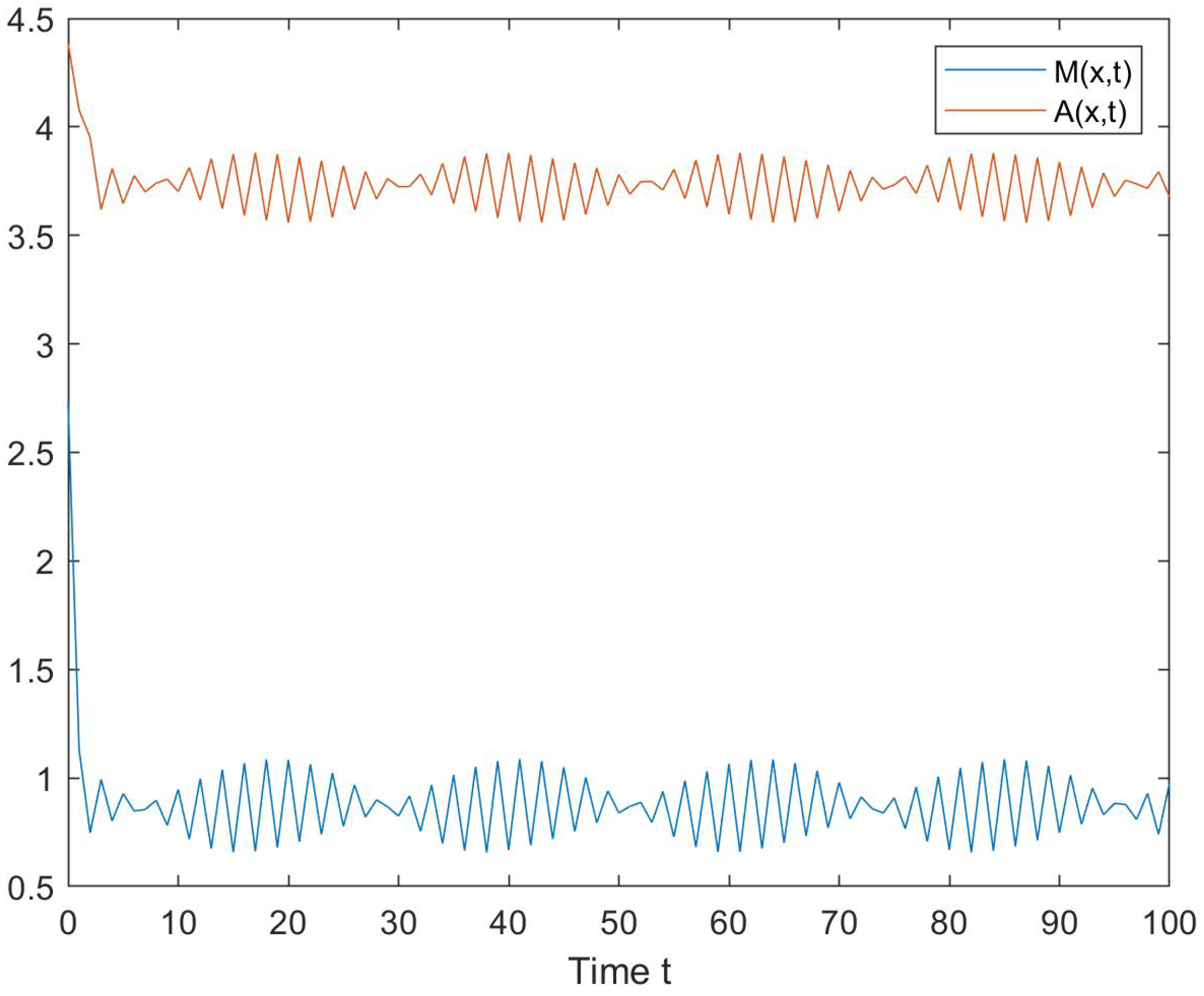
5. Numerical Simulation

Consider the following non-linear diffusion PDE model of IGD

$$\begin{array}{c}\hfill \left\{\begin{array}{cc}\frac{\partial M}{\partial t}=d_1\Delta M+\alpha -\beta MA-{\gamma }_{1}M+\delta A,\hfill & (x,t)\in \Lambda \times {\mathbb{R}}^{+},\hfill \\ \\ \frac{\partial A}{\partial t}=d_2\Delta A+\beta MA-({\gamma }_2+\delta )A,\hfill & (x,t)\in \Lambda \times {\mathbb{R}}^{+},\hfill \\ \frac{\partial M(x,t)}{\partial \overrightarrow{\nu }}=\frac{\partial A(x,t)}{\partial \overrightarrow{\nu }}=0,\hfill & (x,t)\in \partial \Lambda \times {\mathbb{R}}^{+},\hfill \\ M(x,0)={\varphi }_1\left(x\right),A(x,0)={\varphi }_2\left(x\right),\hfill & x\in \Lambda ,\hfill \end{array}\right.\end{array}$$

(22)

where ${\mathbb{R}}^{+}=(0,\infty )$, $\Lambda =(0,10)$, $\alpha =10$, $\beta =6$, ${\gamma }_1=3$ ${\gamma }_2=2$, $\delta =3$, $d_1=0.5$, $d_2=0.8$, ${\varphi }_1\left(x\right)=5+3sin\left(x\right)$, ${\varphi }_2\left(x\right)=7+4cos\left(x\right)$.

A simple calculation gives $5={\gamma }_2+\delta <\alpha \beta {\gamma }_1^{-1}=20$ and $c^{*}=2\sqrt{d_2(\alpha \beta {\gamma }_1^{-1}-{\gamma }_2-\delta )}$ = 8. The condition $\left(\mathrm{A}\right)$ holds. According to Theorem 1 and Theorem 2, for any $c>c^{*}=8$, the model (22) has a traveling wave solution $({\tilde{M}}^{*}\left(\xi \right),{\tilde{A}}^{*}\left(\xi \right))$, which is globally asymptotically stable.

Figure 2 shows that when the initial conditions are the periodic functions ${\varphi }_1\left(x\right)=5+3sin\left(x\right)$ and ${\varphi }_2\left(x\right)=7+4cos\left(x\right)$, the system (22) exists as a globally asymptotically stable oscillatory periodic traveling wave solution.

6. Conclusions

In the last decade, with the popularity of the Internet, the number of Internet users has continued to increase. While people enjoy the convenience and benefits brought by the Internet, some disadvantages brought by the Internet also begin to appear gradually. For example, Internet game addiction endangers the physical and mental health of players. In particular, many young addictive gamers are trapped in it. Many scholars, including mathematicians, have begun to pay attention to and study this phenomenon. Through the analysis of the dynamic change process of Internet gamers, we put forward a new non-linear diffusion PDE model (1) of IGD in this paper. By applying fixed point theory and Lyapunov stability theory, we study the existence and asymptotic stability of the traveling wave of model (1). With the help of the MATLAB toolbox, an example is numerically simulated to examine the correctness of our outcomes. The major findings of the paper provide theoretical help for the research and treatment of Internet game addiction. For example, our results show that appropriate treatment can ensure that the number of gamers is bounded without unlimited increase. The population density of gamers will gradually stabilize at $(\frac{\alpha }{{\gamma }_1},0)$, which suggests that we can eventually make the gamers disappear by reducing the number of moderate gamers and strengthening their treatment. Our work provides an example for applying mathematical theories and methods to solve social problems such as Internet game addiction, which makes the study of this kind of problem transform from qualitative research to quantitative research. In addition, recently published papers [27,28,29,30,31,32,33,34,35,36,37,38,39,40,41,42,43,44,45,46] enlighten us to discuss the existence, exponential stability and Ulam–Hyers stability of model (1) in the sense of fractional calculus in the future.

References

- World Health Organization. The 11th Revision of the International Classification of Diseases (ICD-11). Available online: https://icd.who.int/ (accessed on 25 May 2019).
- Feng, W.; Ramo, D.; Chan, S.; Bourgeois, J. Internet gaming disorder: Trends in prevalence 1998–2016. Addic. Behav. 2017, 75, 17–24. [Google Scholar] [CrossRef] [PubMed]
- American Psychiatric Association, Diagnostic and Statistical Manual of Mental Disorders (DSM-5); American Psychiatric Publishing: Washington, DC, USA, 2013.
- Paulus, F.; Ohmann, S.; von Gontard, A.; Popow, C. Internet gaming disorder in children and adolescents: A systematic review. Dev. Med. Child Neurol. 2018, 60, 645–659. [Google Scholar] [CrossRef] [PubMed]
- Guo, Y.; Li, T. Optimal control and stability analysis of an online game addiction model with two stages. Math. Meth. Appl. Sci. 2020, 43, 4391–4408. [Google Scholar] [CrossRef]
- Li, T.; Guo, Y. Stability and optimal control in a mathematical model of online game addiction. Filomat 2019, 33, 5691–5711. [Google Scholar] [CrossRef] [Green Version]
- Viriyapong, R.; Sookpiam, M. Education campaign and family understanding affect stability and qualitative behavior of an online game addiction model for children and youth in Thailand. Math. Meth. Appl. Sci. 2019, 42, 6906–6916. [Google Scholar] [CrossRef]
- Seno, H. A mathematical model of population dynamics for the internet gaming addiction. Nonlinear Anal-Model. 2021, 26, 861–883. [Google Scholar] [CrossRef]
- Zhao, K. Global stability of a novel nonlinear diffusion online game addiction model with unsustainable control. AIMS Math. 2022, 7, 20752–20766. [Google Scholar] [CrossRef]
- Murray, J. Mathematical Biology; Springer: New York, NY, USA, 1993. [Google Scholar]
- Britton, N. Reaction-Diffusion Equations and Their Applications to Biology; Academic Press: New York, NY, USA, 1986. [Google Scholar]
- Brauer, F.; Castillo-Chavez, C. Mathematical Models in Population Biology and Epidemiology; Springer: New York, NY, USA, 2012. [Google Scholar]
- Diekmann, O. Run for your life, a note on the asymptotic speed of propagation of an epidemic. J. Differ. Equ. 1979, 33, 58–73. [Google Scholar] [CrossRef] [Green Version]
- Abi Rizk, L.; Burie, J.; Ducrot, A. Travelling wave solutions for a nonlocal evolutionary-epidemic system. J. Differ. Equ. 2019, 267, 1467–1509. [Google Scholar] [CrossRef]
- Zhang, Y.; Xu, Z. Dynamics of a diffusive HBV model with delayed Beddington-DeAngelis response. Nonlinear Anal. Real World Appl. 2014, 15, 118–139. [Google Scholar] [CrossRef]
- Ren, X.; Tian, Y.; Liu, L.; Liu, X. A reaction-diffusion within-host HIV model with cell-to-cell transmission. J. Math. Biol. 2018, 76, 1831–1872. [Google Scholar] [CrossRef] [PubMed]
- Kapel, A. Existence of travelling-wave type solutions for the Belousov-Zhabotinskii system of equations. Sib. Mat. Zhurnal 1991, 32, 47–59. [Google Scholar]
- Trofimchuk, E.; Pinto, M.; Trofimchuk, S. On the minimal speed of front propagation in a model of the Belousov-Zhabotinsky reaction. Discrete Contin. Dyn. Syst. Ser. B 2014, 19, 1769–1781. [Google Scholar] [CrossRef]
- Owolabi, K.; Hammouch, Z. Spatiotemporal patterns in the Belousov-Zhabotinskii reaction systems with Atangana-Baleanu fractional order derivative. Phys. A 2019, 523, 1072–1090. [Google Scholar] [CrossRef]
- Alfaro, M.; Coville, J.; Raoul, G. Traveling waves in a nonlocal reaction-diffusion equation as a model for a population structured by a space variable and a phenotypic trait. Commun. Part. Diff. Equ. 2013, 38, 2126–2154. [Google Scholar] [CrossRef]
- Li, J.; Latos, E.; Chen, L. Wavefronts for a nonlinear nonlocal bistable reaction-diffusion equation in population dynamics. J. Differ. Equ. 2017, 263, 6427–6455. [Google Scholar] [CrossRef] [Green Version]
- Diaz, J.; Vrabie, I. Existence for reaction diffusion systems: A compactness method approach. J. Math. Anal. Appl. 1994, 188, 521–540. [Google Scholar] [CrossRef]
- Mallet-Paret, J. The global structure of traveling waves in spatially discrete dynamical systems. J. Dyn. Differ. Equ. 1999, 11, 49–127. [Google Scholar] [CrossRef]
- Guo, Z.; Huang, L.; Zou, X. Impact of discontinuous treatments on disease dynamics in an SIR epidemic model. Math. Biosci. Eng. 2012, 9, 97–110. [Google Scholar]
- Brown, K.; Dunne, P.; Gardner, R. A semilinear parabolic system arising in the theory of superconductivity. J. Differ. Equ. 1981, 40, 232–252. [Google Scholar] [CrossRef] [Green Version]
- Simsen, J.; Gentile, C. On p-Laplacian differential inclusions-Global existence, compactness properties and asymptotic behavior. Nonlinear Anal. 2009, 71, 3488–3500. [Google Scholar] [CrossRef]
- Zhao, K. Stability of a nonlinear ML-nonsingular kernel fractional Langevin system with distributed lags and integral control. Axioms 2022, 11, 350. [Google Scholar] [CrossRef]
- Zhao, K. Existence, stability and simulation of a class of nonlinear fractional Langevin equations involving nonsingular Mittag—Leffler kernel. Fractal Fract. 2022, 6, 469. [Google Scholar] [CrossRef]
- Zhao, K.; Ma, Y. Study on the existence of solutions for a class of nonlinear neutral Hadamard-type fractional integro-differential equation with infinite delay. Fractal Fract. 2021, 5, 52. [Google Scholar] [CrossRef]
- Zhao, K. Stability of a nonlinear fractional Langevin system with nonsingular exponential kernel and delay Control. Discrete Dyn. Nat. Soc. 2022, 2022, 9169185. [Google Scholar] [CrossRef]
- Zhao, K. Local exponential stability of four almost-periodic positive solutions for a classic Ayala-Gilpin competitive ecosystem provided with varying-lags and control terms. Int. J. Control, 2022; in press. [Google Scholar] [CrossRef]
- Zhao, K. Local exponential stability of several almost periodic positive solutions for a classical controlled GA-predation ecosystem possessed distributed delays. Appl. Math. Comput. 2023, 437, 127540. [Google Scholar] [CrossRef]
- Huang, H.; Zhao, K.; Liu, X. On solvability of BVP for a coupled Hadamard fractional systems involving fractional derivative impulses. AIMS Math. 2022, 7, 19221–19236. [Google Scholar] [CrossRef]
- Zhao, K.; Ma, S. Ulam-Hyers-Rassias stability for a class of nonlinear implicit Hadamard fractional integral boundary value problem with impulses. AIMS Math. 2021, 7, 3169–3185. [Google Scholar] [CrossRef]
- Zhao, K.; Deng, S. Existence and Ulam-Hyers stability of a kind of fractional-order multiple point BVP involving noninstantaneous impulses and abstract bounded operator. Adv. Differ. Equ-NY 2021, 2021, 44. [Google Scholar] [CrossRef]
- Luo, D.; Tian, M.; Zhu, Q. Some results on finite-time stability of stochastic fractional-order delay differential equations. Chaos Soliton Fract. 2022, 158, 111996. [Google Scholar] [CrossRef]
- Wang, X.; Luo, D.; Zhu, Q. Ulam-Hyers stability of Caputo type fuzzy fractional differential equations with time-delays. Chaos Soliton Fract. 2022, 156, 111822. [Google Scholar] [CrossRef]
- Luo, D.; Zhu, Q.; Luo, Z. A novel result on averaging principle of stochastic Hilfer-type fractional system involving non-Lipschitz coefficients. Appl. Math. Lett. 2021, 122, 107549. [Google Scholar] [CrossRef]
- Luo, D.; Zhu, Q.; Luo, Z. An averaging principle for stochastic fractional differential equations with time-delays. Appl. Math. Lett. 2020, 105, 106290. [Google Scholar] [CrossRef]
- Zhang, T.; Xiong, L. Periodic motion for impulsive fractional functional differential equations with piecewise Caputo derivative. Appl. Math. Lett. 2020, 101, 106072. [Google Scholar] [CrossRef]
- Zhang, T.; Zhou, J.; Liao, Y. Exponentially stable periodic oscillation and Mittag-Leffler stabilization for fractional-order impulsive control neural networks with piecewise Caputo derivatives. IEEE Trans. Cybernet. 2022, 52, 9670–9683. [Google Scholar] [CrossRef]
- Zhang, T.; Li, Y. Exponential Euler scheme of multi-delay Caputo-Fabrizio fractional-order differential equations. Appl. Math. Lett. 2022, 124, 107709. [Google Scholar] [CrossRef]
- Zhang, T.; Li, Y. Global exponential stability of discrete-time almost automorphic Caputo-Fabrizio BAM fuzzy neural networks via exponential Euler technique. Knowl-Based Syst. 2022, 246, 108675. [Google Scholar] [CrossRef]
- Li, Z.; Zhang, W.; Huang, C.; Zhou, J. Bifurcation for a fractional-order Lotka-Volterra predator-prey model with delay feedback control. AIMS Math. 2021, 6, 675–687. [Google Scholar]
- Zhou, J.; Zhou, B.; Tian, L.; Wang, Y. Variational approach for the variable-order fractional magnetic Schrödinger equation with variable growth and steep potential in ℝN*. Adv. Math. Phys. 2020, 2020, 1320635. [Google Scholar] [CrossRef]
- Zhou, J.; Zhou, B.; Wang, Y. Multiplicity results for variable-order nonlinear fractional magnetic Schrödinger equation with variable growth. J. Funct. Spaces 2020, 2020, 7817843. [Google Scholar] [CrossRef]
Figure 1.
General scheme of the state transition of Internet gamers in our modeling.
Figure 2.
Evolutions of and over time t.
Publisher’s Note: MDPI stays neutral with regard to jurisdictional claims in published maps and institutional affiliations. |
© 2022 by the author. Licensee MDPI, Basel, Switzerland. This article is an open access article distributed under the terms and conditions of the Creative Commons Attribution (CC BY) license (https://creativecommons.org/licenses/by/4.0/).
Share and Cite
MDPI and ACS Style
Zhao, K. Probing the Oscillatory Behavior of Internet Game Addiction via Diffusion PDE Model. Axioms 2022, 11, 649. https://doi.org/10.3390/axioms11110649
AMA Style
Zhao K. Probing the Oscillatory Behavior of Internet Game Addiction via Diffusion PDE Model. Axioms. 2022; 11(11):649. https://doi.org/10.3390/axioms11110649
Chicago/Turabian StyleZhao, Kaihong. 2022. "Probing the Oscillatory Behavior of Internet Game Addiction via Diffusion PDE Model" Axioms 11, no. 11: 649. https://doi.org/10.3390/axioms11110649
Note that from the first issue of 2016, this journal uses article numbers instead of page numbers. See further details here.