
New Financial Ratios Based on the Compositional Data Methodology
 ,
, 
Abstract
:1. Introduction
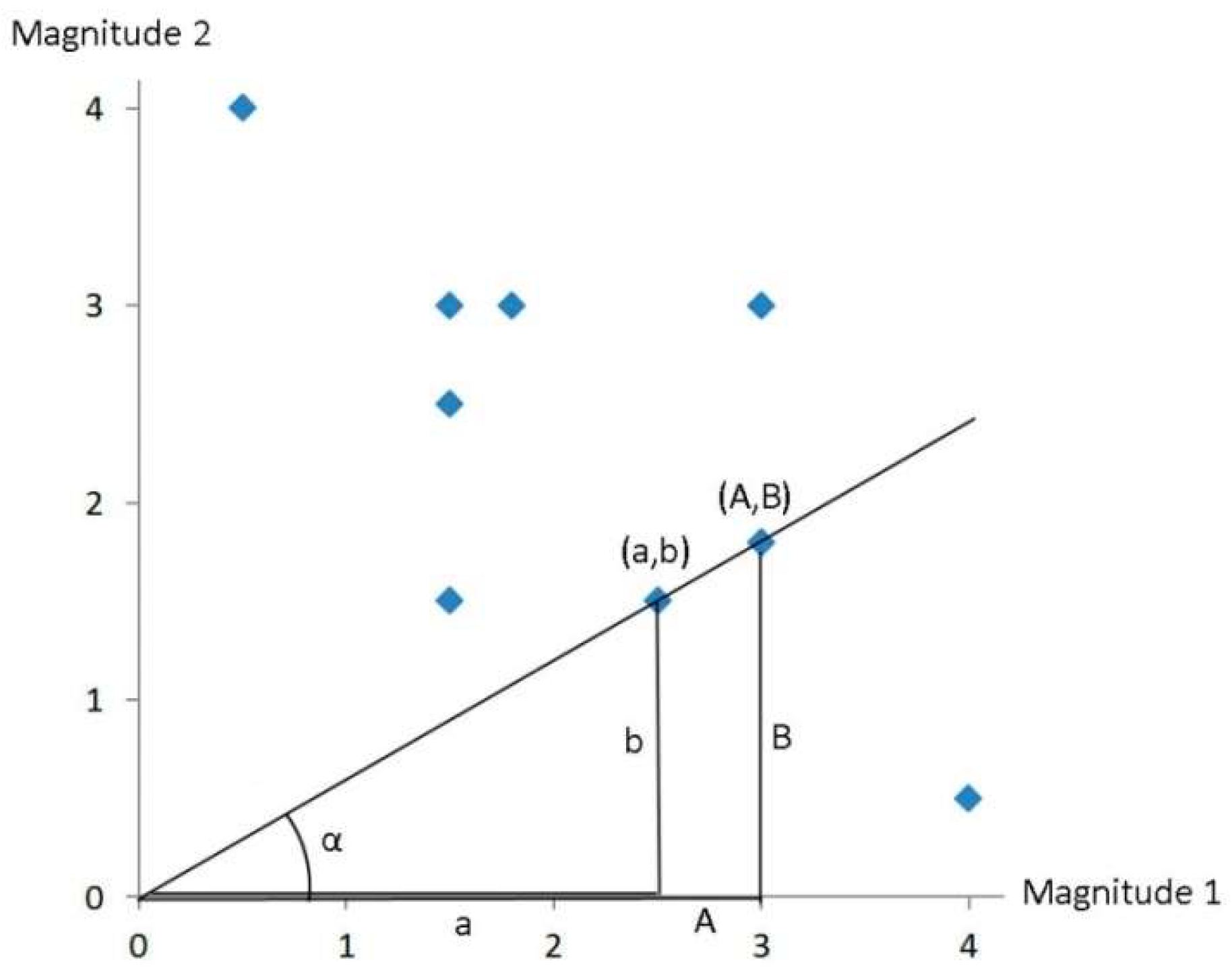
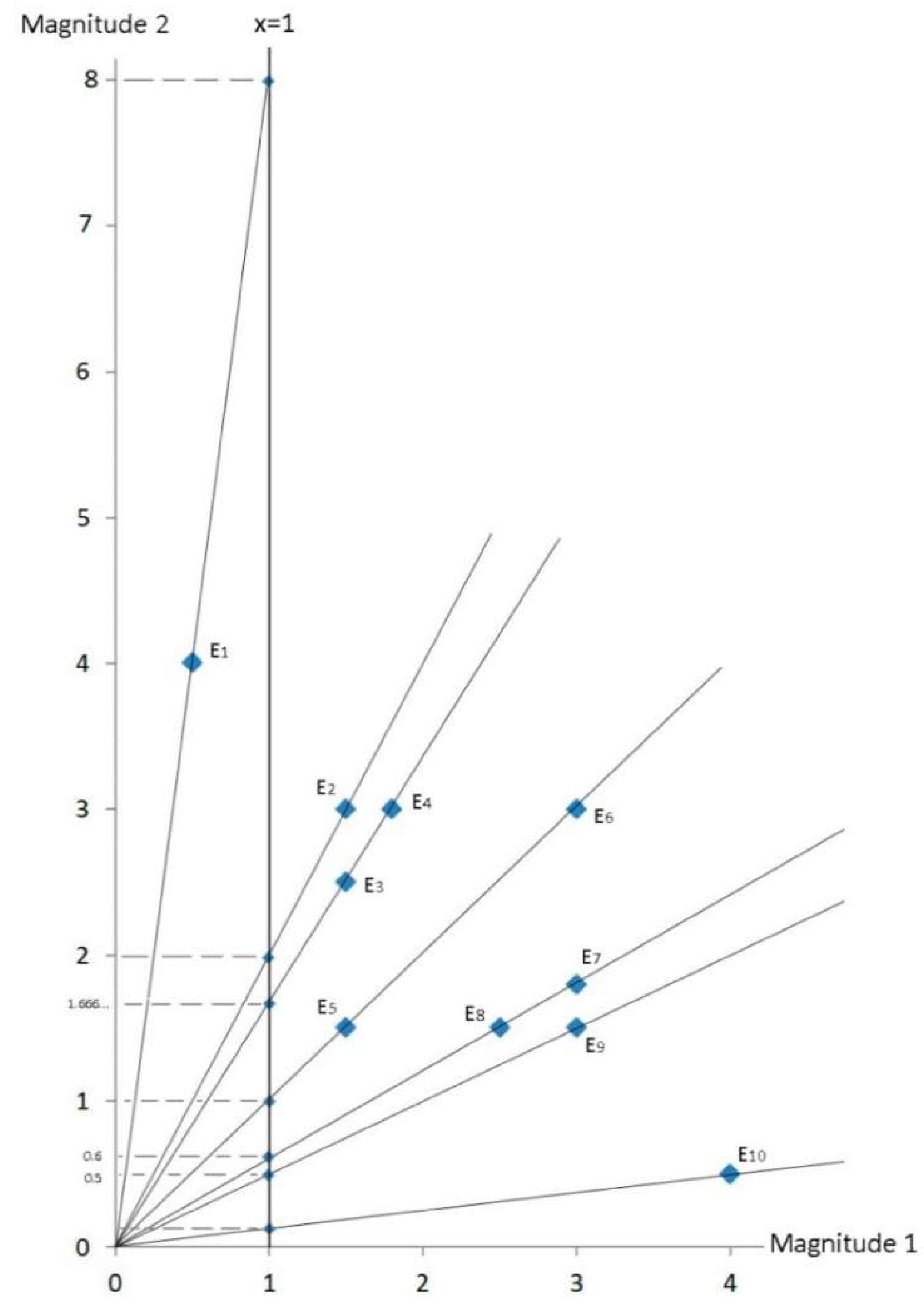
2. Theory: The Problem of the Asymmetry of Standard Ratios and the Appearance of Spurious Outliers
3. Materials and Methods
3.1. Financial Ratios Based on the CoDa Methodology

- The same values identifiable as outliers in both cases are obtained.
- The same skewness statistic is obtained, but with the opposite sign.
- The relationships with non-financial external variables (e.g., differences in means, correlations, coefficients of regression) are identical in size, but with opposite signs.
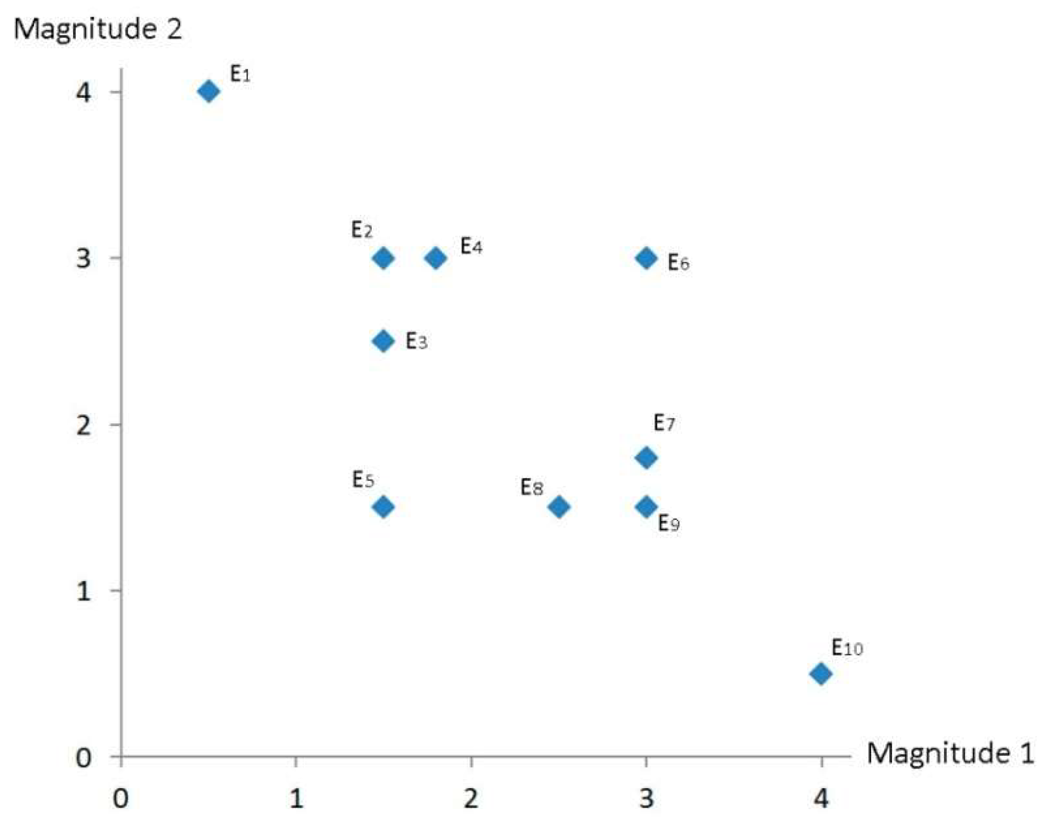
3.2. Example Data
4. Results
5. Discussion
6. Conclusions
Author Contributions
Funding
Data Availability Statement
Conflicts of Interest
References
- Barnes, P. The analysis and use of financial ratios: A review article. J. Bus. Financ. Account. 1987, 14, 449–461. [Google Scholar] [CrossRef]
- Bernstein, L.A. Financial Statement Analysis: Theory, Application and Interpretation; Irwin: Homewood, IL, UAS, 1993; pp. 1–1075. [Google Scholar]
- Gallizo, J.L. Avances en la investigación de ratios financieros. La dinámica de los ratios. Rev. De Contab. Y Dir. 2005, 2, 21–146. [Google Scholar]
- Whittington, G. Some basic properties of accounting ratios. J. Bus. Financ. Account. 1980, 7, 219–223. [Google Scholar] [CrossRef]
- Cowen, S.S.; Hoffer, J.A. Usefulness of financial ratios in a single industry. J. Bus. Res. 1982, 10, 103–118. [Google Scholar] [CrossRef]
- Deakin, E.B. Distributions of financial accounting ratios: Some empirical evidence. Account. Rev. 1976, 51, 90–96. [Google Scholar]
- Lev, B.; Sunder, S. Methological issues in the use of financial ratios. J. Account. Econ. 1979, 1, 187–210. [Google Scholar] [CrossRef]
- Mcleay, S.; Omar, A. The sensitivity of prediction models to the non-normality of bounded and unbounded financial ratios. Br. Account. Rev. 2000, 32, 213–230. [Google Scholar] [CrossRef]
- Delord, B.; Montaigne, É.; Coelho, A. Vine planting rights, farm size and economic performance: Do economies of scale matter in the French viticulture sector? Wine Econ. Policy 2015, 4, 22–34. [Google Scholar] [CrossRef]
- Fernandez-Olmosá, M.; Rosell-Martinez, J.; Espitia-Escuer, M.A. Vertical integration in the wine industry: A transaction costs analysis on the Rioja DOCa. Agribusiness 2009, 25, 231–250. [Google Scholar] [CrossRef]
- Hammervoll, T.; Mora, P.; Toften, K. The financial crisis and the wine industry: The performance of niche firms versus mass-market firms. Wine Econ. Policy 2014, 3, 108–114. [Google Scholar] [CrossRef] [Green Version]
- Lorenzo, J.R.F.; Rubio, M.T.M.; Garcés, S.A. The competitive advantage in business, capabilities and strategy. What general performance factors are found in the Spanish wine industry? Wine Econ. Policy 2018, 7, 94–108. [Google Scholar] [CrossRef]
- Newton, S.K.; Gilinsky, A., Jr.; Jordan, D. Differentiation strategies and winery financial performance: An empirical investigation. Wine Econ. Policy 2015, 4, 88–97. [Google Scholar] [CrossRef]
- Tseng, S.H.; Nguyen, T.S. A method for visualizing posterior probit model uncertainty in the early prediction of fraud for sustainability development. Axioms 2021, 10, 178. [Google Scholar] [CrossRef]
- Isles, P.D. The misuse of ratios in ecological stoichiometry. Ecology 2020, 101, e03153. [Google Scholar] [CrossRef]
- Creixans-Tenas, J.; Coenders, G.; Arimany-Serrat, N. Corporate social responsibility and financial profile of Spanish private hospitals. Heliyon 2019, 5, e02623. [Google Scholar] [CrossRef] [Green Version]
- Ezzamel, M.; Mar-Molinero, C. The distributional properties of financial ratios in UK manufacturing companies. J. Bus. Financ. Account. 1990, 17, 1–29. [Google Scholar] [CrossRef]
- Martikainen, T.; Perttunen, J.; Yli-Olli, P.; Gunasekaran, A. Financial ratio distribution irregularities: Implications for ratio classification. Eur. J. Oper. Res. 1995, 80, 34–44. [Google Scholar] [CrossRef]
- So, J.C. Some empirical evidence on the outliers and the non-normal distribution of financial ratios. J. Bus. Financ. Account. 1987, 14, 483–496. [Google Scholar] [CrossRef]
- Watson, C.J. Multivariate distributional properties, outliers, and transformation of financial ratios. Account. Rev. 1990, 65, 682–695. [Google Scholar]
- Frecka, T.J.; Hopwood, W.S. The effects of outliers on the cross-sectional distributional properties of financial ratios. Account. Rev. 1983, 58, 115–128. [Google Scholar]
- Linares-Mustarós, S.; Coenders, G.; Vives-Mestres, M. Financial performance and distress profiles. From classification according to financial ratios to compositional classification. Adv. Account. 2018, 40, 1–10. [Google Scholar] [CrossRef]
- Aitchison, J. The Statistical Analysis of Compositional Data. Monographs on Statistics and Applied Probability; Chapman and Hall: London, UK, 1986; pp. 1–416. [Google Scholar]
- Filzmoser, P.; Hron, K.; Templ, M. Applied Compositional Data Analysis with Worked Examples in R.; Springer: New York, NY, USA, 2018; pp. 1–280. [Google Scholar]
- Greenacre, M. Compositional Data Analysis in Practice; Chapman and Hall/CRC Press: New York, NY, USA, 2018; pp. 1–121. [Google Scholar]
- Pawlowsky-Glahn, V.; Buccianti, A. Compositional Data Analysis. Theory and Applications; Wiley: New York, NY, USA, 2011; pp. 1–378. [Google Scholar]
- Pawlowsky-Glahn, V.; Egozcue, J.J.; Tolosana-Delgado, R. Modeling and Analysis of Compositional Data; Wiley: Chichester, UK, 2015; pp. 1–247. [Google Scholar]
- van den Boogaart, K.G.; Tolosana-Delgado, R. Analyzing Compositional Data with R.; Springer: Berlin/Heidelberg, Germany, 2013; pp. 1–258. [Google Scholar]
- Aitchison, J. The statistical analysis of compositional data (with discussion). J. R. Stat. Soc. Ser. B Stat. Methodol. 1982, 44, 139–177. [Google Scholar] [CrossRef]
- Coenders, G.; Ferrer-Rosell, B. Compositional data analysis in tourism. Review and future directions. Tour. Anal. 2020, 25, 153–168. [Google Scholar] [CrossRef]
- Belles-Sampera, J.; Guillen, M.; Santolino, M. Compositional methods applied to capital allocation problems. J. Risk 2016, 19, 15–30. [Google Scholar] [CrossRef]
- Boonen, T.; Guillén, M.; Santolino, M. Forecasting compositional risk allocations. Insur. Math. Econ. 2019, 84, 79–86. [Google Scholar] [CrossRef] [Green Version]
- Davis, B.C.; Hmieleski, K.M.; Webb, J.W.; Coombs, J.E. Funders’ positive affective reactions to entrepreneurs’ crowdfunding pitches: The influence of perceived product creativity and entrepreneurial passion. J. Bus. Ventur. 2017, 32, 90–106. [Google Scholar] [CrossRef]
- Gámez-Velázquez, D.; Coenders, G. Identification of exchange rate shocks with compositional data and written press. Financ. Mark. Valuat. 2020, 6, 99–113. [Google Scholar] [CrossRef]
- Kokoszka, P.; Miao, H.; Petersen, A.; Shang, H.L. Forecasting of density functions with an application to cross-sectional and intraday returns. Int. J. Forecast. 2019, 35, 1304–1317. [Google Scholar] [CrossRef]
- Ortells, R.; Egozcue, J.J.; Ortego, M.I.; Garola, A. Relationship between popularity of key words in the Google browser and the evolution of worldwide financial indices. In Compositional Data Analysis. Springer Proceedings in Mathematics & Statistics; Martín-Fernández, J.A., Thió-Henestrosa, S., Eds.; Springer: Cham, Switzerland, 2016; Volume 187, pp. 145–166. [Google Scholar]
- Maldonado, W.L.; Egozcue, J.J.; Pawlowsky–Glahn, V. No-arbitrage matrices of exchange rates: Some characterizations. Int. J. Econ. Theory 2021, 17, 375–389. [Google Scholar] [CrossRef]
- Maldonado, W.L.; Egozcue, J.J.; Pawlowsky–Glahn, V. Compositional analysis of exchange rates. In Advances in Contemporary Statistics and Econometrics. Festschrift in Honor of Christine Thomas-Agnan; Daouia, A., Ruiz-Gazen, A., Eds.; Springer Nature: Cham, Switzerland, 2021; pp. 489–507. [Google Scholar] [CrossRef]
- Porro, F. A geographical analysis of the systemic risk by a compositional data (CoDa) Approach. In Mathematical and Statistical Methods for Actuarial Sciences and Finance; Corazza, M., Perna, C., Pizzi, C., Sibillo, M., Eds.; Springer: Cham, Switzerland, 2022; pp. 383–389. [Google Scholar] [CrossRef]
- Vega-Baquero, J.D.; Santolino, M. Too big to fail? an analysis of the Colombian banking system through compositional data. LAJCB 2022, 3, 100060. [Google Scholar] [CrossRef]
- Verbelen, R.; Antonio, K.; Claeskens, G. Unravelling the predictive power of telematics data in car insurance pricing. J. R. Stat. Soc. Ser. C Appl. Stat. 2018, 67, 1275–1304. [Google Scholar] [CrossRef] [Green Version]
- Voltes-Dorta, A.; Jiménez, J.L.; Suárez-Alemán, A. An initial investigation into the impact of tourism on local budgets: A comparative analysis of Spanish municipalities. Tour. Manag. 2014, 45, 124–133. [Google Scholar] [CrossRef]
- Wang, H.; Lu, S.; Zhao, J. Aggregating multiple types of complex data in stock market prediction: A model-independent framework. Knowl. Based Syst. 2019, 164, 193–204. [Google Scholar] [CrossRef] [Green Version]
- Arimany-Serrat, N.; Farreras-Noguer, M.À.; Coenders, G. New developments in financial statement analysis. Liquidity in the winery sector. Accounting 2022, 8, 355–366. [Google Scholar] [CrossRef]
- Carreras-Simó, M.; Coenders, G. Principal component analysis of financial statements. A compositional approach. Rev. Métodos Cuantitativos Econ. Empresa 2020, 29, 18–37. [Google Scholar] [CrossRef]
- Carreras-Simó, M.; Coenders, G. The relationship between asset and capital structure: A compositional approach with panel vector autoregressive models. Quant. Financ. Econ. 2021, 5, 571–590. [Google Scholar] [CrossRef]
- Jofre-Campuzano, P.; Coenders, G. Compositional classification of financial statement profiles: The weighted case. J. Risk Financ. Manag. 2022, 15, 546. [Google Scholar] [CrossRef]
- Saus-Sala, E.; Farreras-Noguer, M.A.; Arimany-Serrat, N.; Coenders, G. Compositional DuPont analysis. A visual tool for strategic financial performance assessment. In Advances in Compositional Data Analysis. Festschrift in Honour of Vera Pawlowsky-Glahn; Filzmoser, P., Hron, K., Martín-Fernández, J.A., Palarea-Albaladejo, J., Eds.; Springer Nature: Cham, Switzerland, 2021; pp. 189–206. [Google Scholar] [CrossRef]
- Chen, K.H.; Shimerda, T.A. An empirical analysis of useful financial ratios. Financ. Manag. 1981, 10, 51–60. [Google Scholar] [CrossRef]
- Buccianti, A.; Mateu-Figueras, G.; Pawlowsky-Glahn, V. Compositional Data Analysis in the Geosciences: From Theory to Practice; Geological Society of London: London, UK, 2006; pp. 1–212. [Google Scholar]
- Egozcue, J.J.; Pawlowsky-Glahn, V. Compositional data: The sample space and its structure. TEST 2019, 28, 599–638. [Google Scholar] [CrossRef]
- Egozcue, J.J.; Pawlowsky-Glahn, V.; Mateu-Figueras, G.; Barcelo-Vidal, C. Isometric logratio transformations for compositional data analysis. Math Geol. 2003, 35, 279–300. [Google Scholar] [CrossRef]
- Vizcaino, D.; Domínguez, A.; Sosa, J. Importancia Económica y Social del Sector Vitivinícola en España; Organización Interprofesional del Vino en España: Madrid, Spain, 2020; pp. 1–64. Available online: https://www.agro-alimentarias.coop/ficheros/doc/06306.pdf (accessed on 1 March 2022).
- Feranecová, A.; Krigovská, A. Measuring the performance of universities through cluster analysis and the use of financial ratio indexes. Econ. Sociol. 2016, 9, 259–271. [Google Scholar] [CrossRef]
- Santis, P.; Albuquerque, A.; Lizarelli, F. Do sustainable companies have a better financial performance? A study on Brazilian public companies. J. Clean. Prod. 2016, 133, 735–745. [Google Scholar] [CrossRef]
- Yoshino, N.; Taghizadeh-Hesary, F.; Charoensivakorn, P.; Niraula, B. Small and medium-sized enterprise (SME) credit risk analysis using bank lending data: An analysis of Thai SMEs. J. Comp. Asian Dev. 2016, 15, 383–406. [Google Scholar] [CrossRef]
- Rondós Casas, E.; Linares-Mustarós, S.; Farreras-Noguer, M.A. Expansion of the current methodology for the study of the short-term liquidity problems in a sector. Intang. Cap. 2018, 14, 25–34. [Google Scholar] [CrossRef] [Green Version]
- Aitchison, J. Principal component analysis of compositional data. Biometrika 1983, 70, 57–65. [Google Scholar] [CrossRef]
- Stevens, S.S. On the theory of scales of measurement. Science 1946, 103, 677–680. [Google Scholar] [CrossRef]
- Martín-Fernández, J.A.; Hron, K.; Templ, M.; Filzmoser, P.; Palarea-Albaladejo, J. Model-based replacement of rounded zeros in compositional data: Classical and robust approaches. Comput. Stat. Data. Anal. 2012, 56, 2688–2704. [Google Scholar] [CrossRef]
- Palarea-Albaladejo, J.; Martín-Fernández, J.A. A modified EM alr-algorithm for replacing rounded zeros in compositional data sets. Comput. Geosci. 2008, 34, 2233–2251. [Google Scholar] [CrossRef]
- Palarea-Albaladejo, J.; Martín-Fernández, J.A. zCompositions—R package for multivariate imputation of left-censored data under a compositional approach. Chemom. Intell. Lab. Syst. 2015, 143, 85–96. [Google Scholar] [CrossRef]


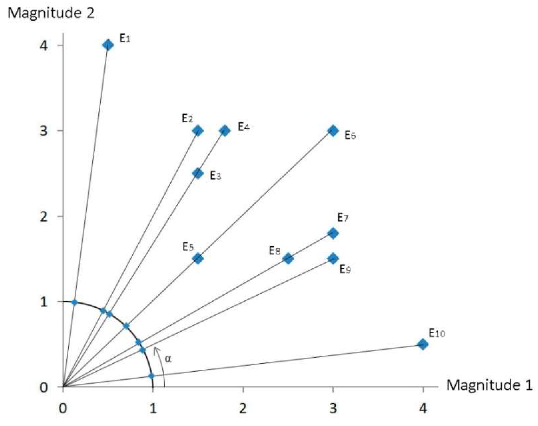
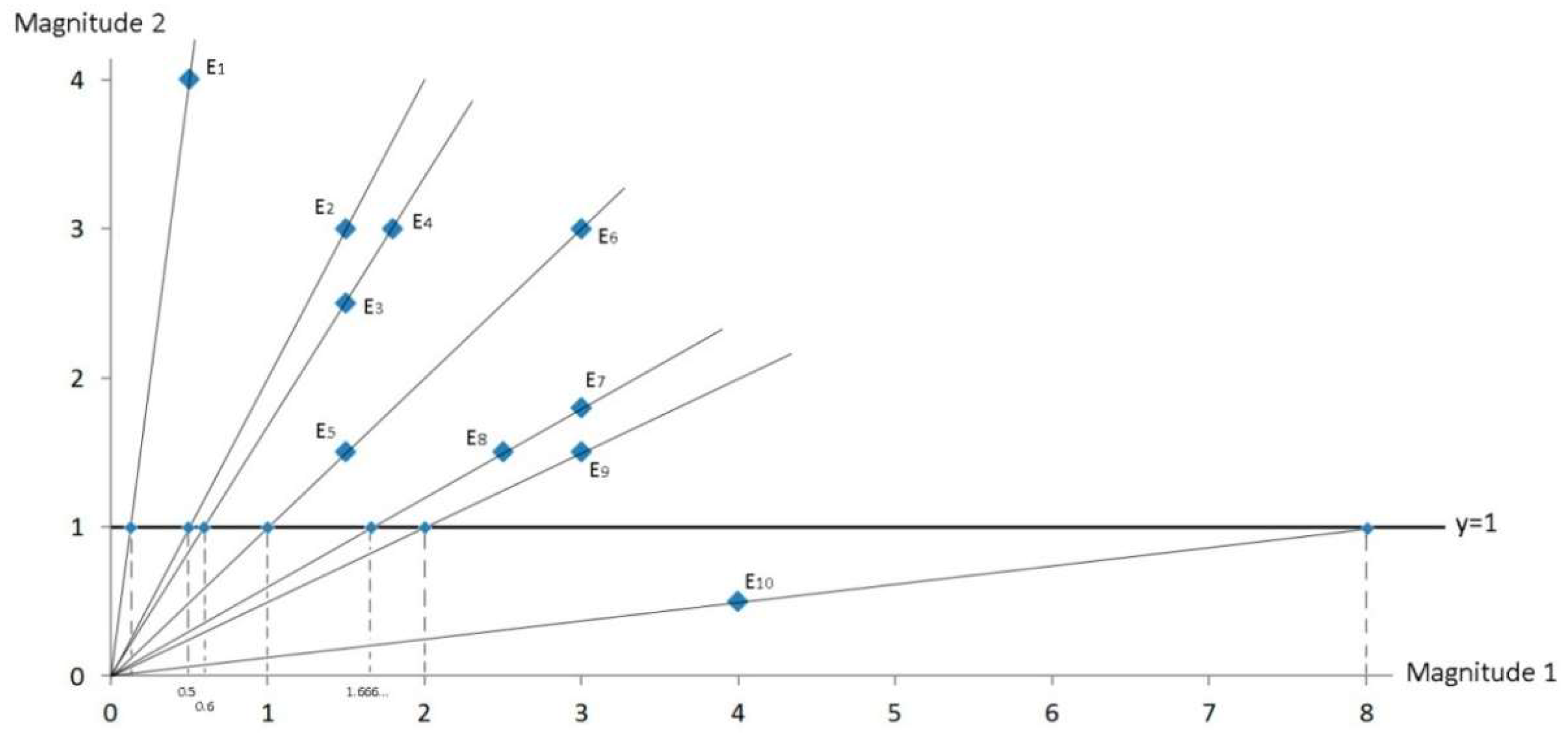
| Magnitude 1 | Magnitude 2 | α | |||
|---|---|---|---|---|---|
| Firm E1 | 0.5 | 4 | ~82.875 (=45 + 37.875) | 8 | 0.125 |
| Firm E2 | 1.5 | 3 | ~63.435 (=45 + 18.435) | 2 | 0.5 |
| Firm E3 | 1.5 | 2.5 | ~59.035 (=45 + 14.035) | 0.6 | |
| Firm E4 | 1.8 | 3 | ~59.035 (=45 + 14.035) | 0.6 | |
| Firm E5 | 1.5 | 1.5 | ~45 (=45 + 0) | 1 | 1 |
| Firm E6 | 3 | 3 | ~45 (=45 − 0) | 1 | 1 |
| Firm E7 | 3 | 1.8 | ~30.965 (=45 − 14.035) | 0.6 | |
| Firm E8 | 2.5 | 1.5 | ~30.965 (=45 − 14.035) | 0.6 | |
| Firm E9 | 3 | 1.5 | ~26.565 (=45 − 18.435) | 0.5 | 2 |
| Firm E10 | 4 | 0.5 | ~7.125 (=45 − 37.875) | 0.125 | 8 |
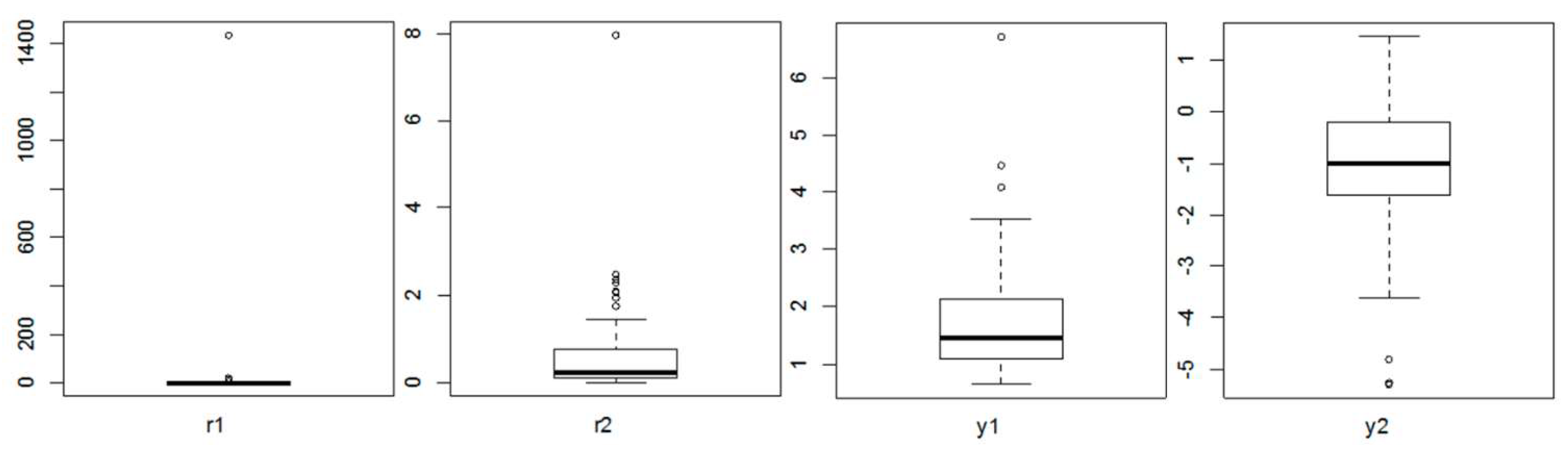
| Skewness | Kurtosis | n Outliers * | n Extreme Outliers ** | |
|---|---|---|---|---|
| r1 | 10.48 | 109.87 | 10 | 7 |
| r2 | 5.27 | 38.85 | 9 | 1 |
| y1 | 1.97 | 6.53 | 3 | 1 |
| y2 | −0.98 | 1.52 | 3 | 0 |
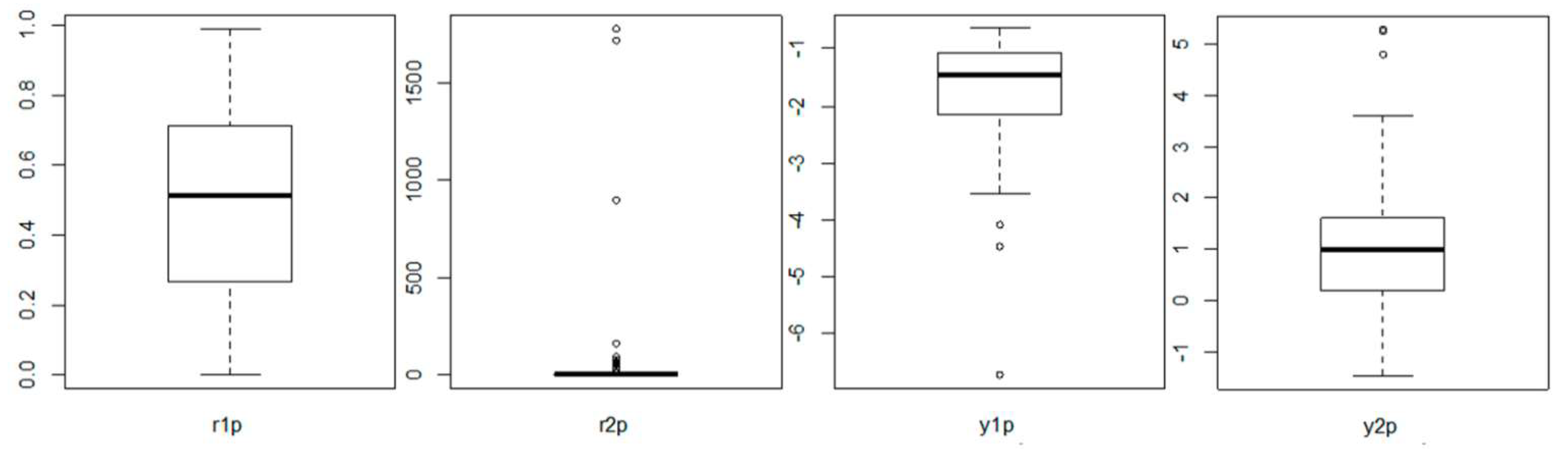
| r1p | −0.01 | −1.16 | 0 | 0 |
| r2p | 6.34 | 40.72 | 22 | 17 |
| y1p | −1.97 | 6.53 | 3 | 1 |
| y2p | 0.98 | 1.52 | 3 | 0 |
| t-Value | p-Value | R-Squared | |
|---|---|---|---|
| r1 | 0.53 | 0.59 | 0.3% |
| r2 | 1.88 | 0.06 * | 3.2% |
| y1 | 0.25 | 0.80 | 0.1% |
| y2 | 2.14 | 0.03 ** | 4.1% |
| r1p | −2.23 | 0.03 ** | 4.4% |
| r2p | −0.78 | 0.44 | 0.6% |
| y1p | −0.25 | 0.80 | 0.1% |
| y2p | −2.14 | 0.03 ** | 4.1% |
Publisher’s Note: MDPI stays neutral with regard to jurisdictional claims in published maps and institutional affiliations. |
© 2022 by the authors. Licensee MDPI, Basel, Switzerland. This article is an open access article distributed under the terms and conditions of the Creative Commons Attribution (CC BY) license (https://creativecommons.org/licenses/by/4.0/).
Share and Cite
Linares-Mustarós, S.; Farreras-Noguer, M.À.; Arimany-Serrat, N.; Coenders, G. New Financial Ratios Based on the Compositional Data Methodology. Axioms 2022, 11, 694. https://doi.org/10.3390/axioms11120694
Linares-Mustarós S, Farreras-Noguer MÀ, Arimany-Serrat N, Coenders G. New Financial Ratios Based on the Compositional Data Methodology. Axioms. 2022; 11(12):694. https://doi.org/10.3390/axioms11120694
Chicago/Turabian StyleLinares-Mustarós, Salvador, Maria Àngels Farreras-Noguer, Núria Arimany-Serrat, and Germà Coenders. 2022. "New Financial Ratios Based on the Compositional Data Methodology" Axioms 11, no. 12: 694. https://doi.org/10.3390/axioms11120694