
HPSBA: A Modified Hybrid Framework with Convergence Analysis for Solving Wireless Sensor Network Coverage Optimization Problem

Abstract
:1. Introduction
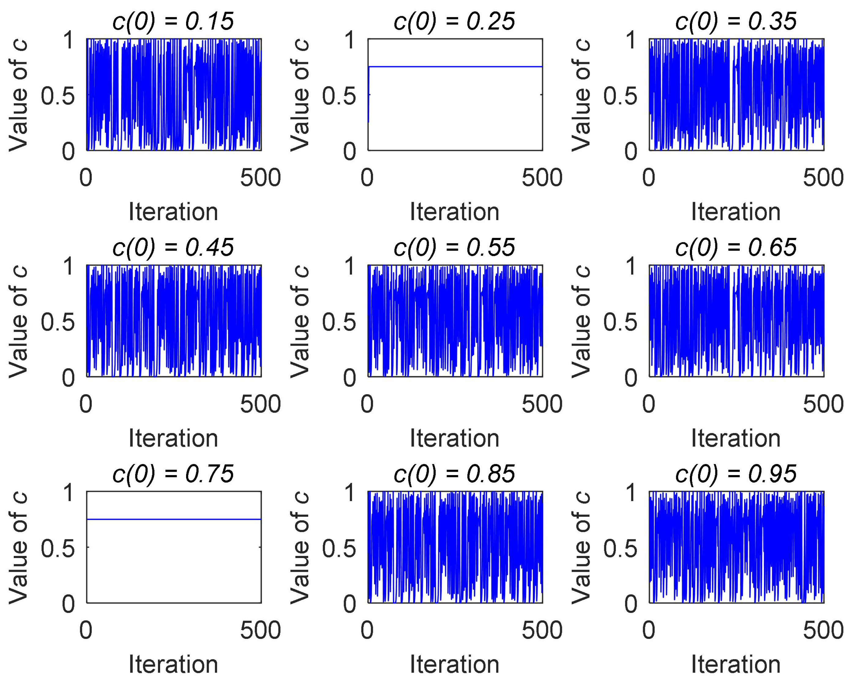
- A novel hybrid particle swarm butterfly algorithm is proposed. This combination strikes a balance between exploitation and exploration. We design that the control strategy of parameter c is based on Logistic map, and the parameter is based on adaptive adjustment strategy of the HPSBA for improving the optimization speed, convergence accuracy and global search capability. Moreover, the individual scent intensity value is calculated with absolute value of the proposed HPSBA.
- To ensure that the proposed algorithm works, we compare the optimization results of twenty-six benchmark functions with ten intelligent optimization algorithms. According to the mean value (Mean), standard deviation (Std), Wilcoxon rank-sum (WRS) test findings, and convergence curves, the simulation results show that HPSBA has a competitive overall performance.
- The node optimization coverage problem of the WSN is solved using the proposed HPSBA. The application and advantages of the HPSBA are also discussed.
2. Basic Knowledge
2.1. Particle Swarm Optimization
2.2. Butterfly Optimization Algorithm
2.3. Node Coverage Optimization Problem Model
3. Method
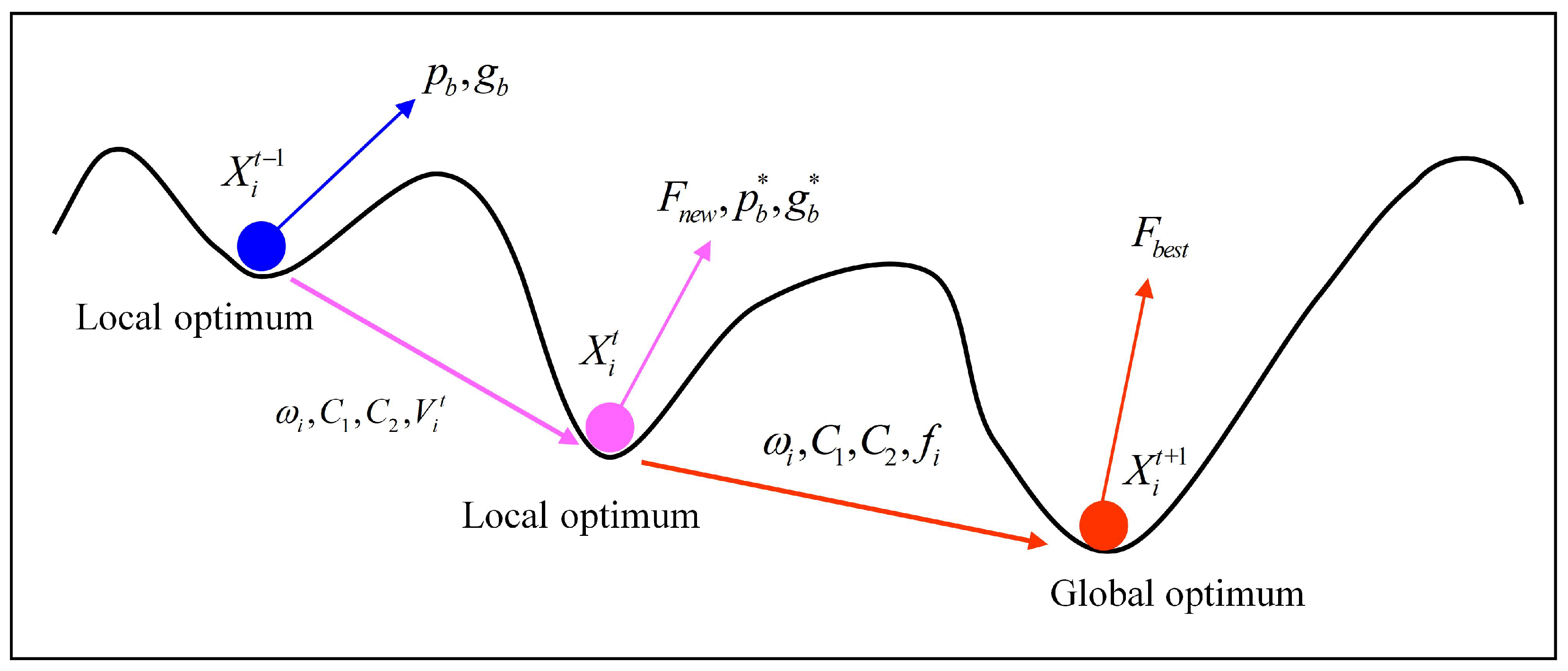
3.1. Hybrid Particle Swarm Butterfly Algorithm (HPSBA)
3.1.1. Algorithmic Population Initialization
3.1.2. Algorithmic Exploration
3.1.3. Algorithmic Exploitation
3.1.4. The Chaotic Adjusting Strategies
3.2. Complexity Analysis of the HPSBA
3.2.1. Time Complexity
3.2.2. Space Complexity
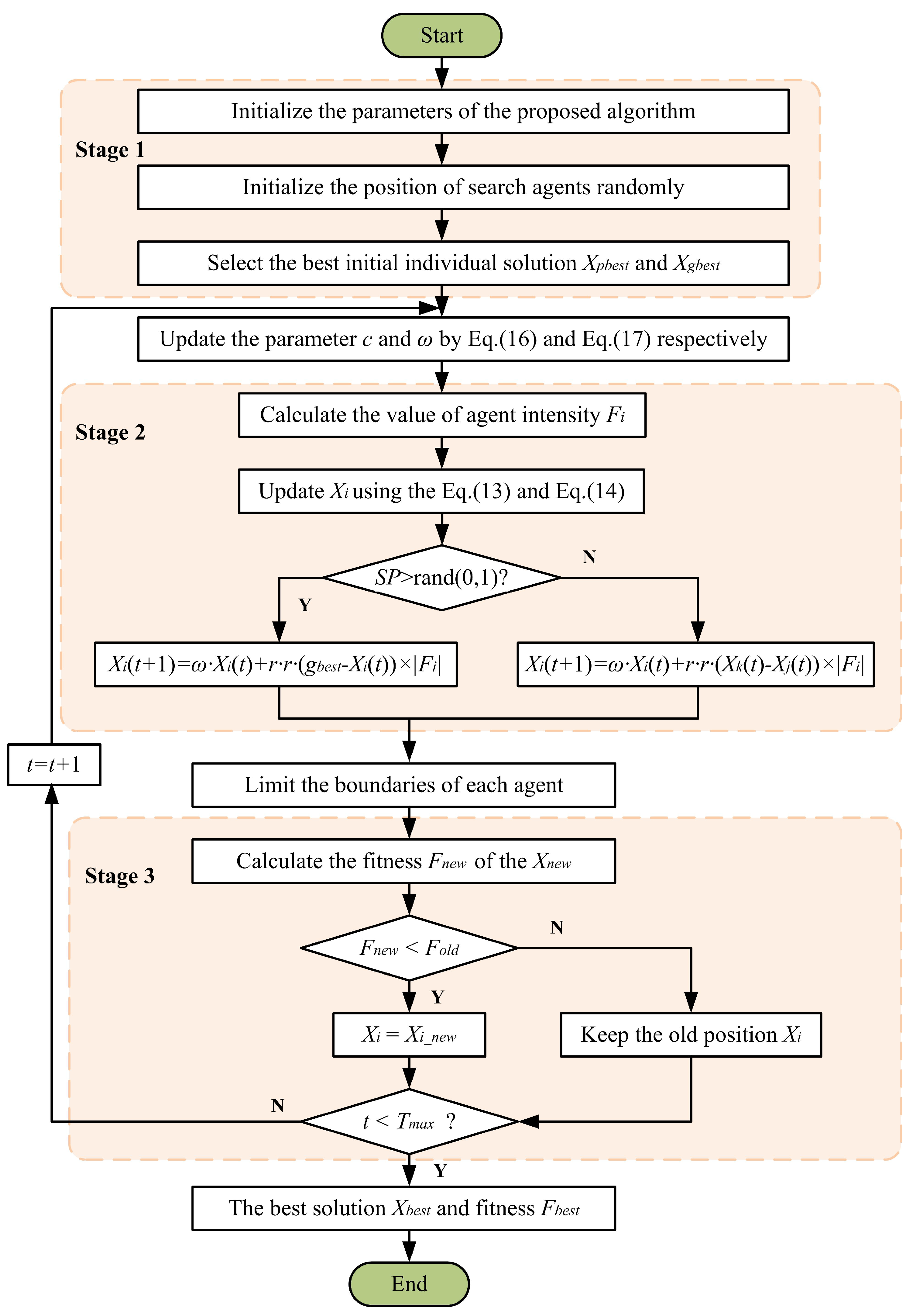
3.3. The Pseudo-Code and Flowchart of the HPSBA
| Algorithm 1: Pseudo-code of HPSBA |
 |
3.4. Convergence Analysis of the HPSBA
3.4.1. Convergence Criterion
3.4.2. Convergence Analysis
4. Analyses and Results of Numerical Optimization
4.1. Parameter Setting of Comparison Algorithms
4.2. Comparison Results of HPSBA with Others (Dim = 30)
4.2.1. Analysis of the Numerical Results
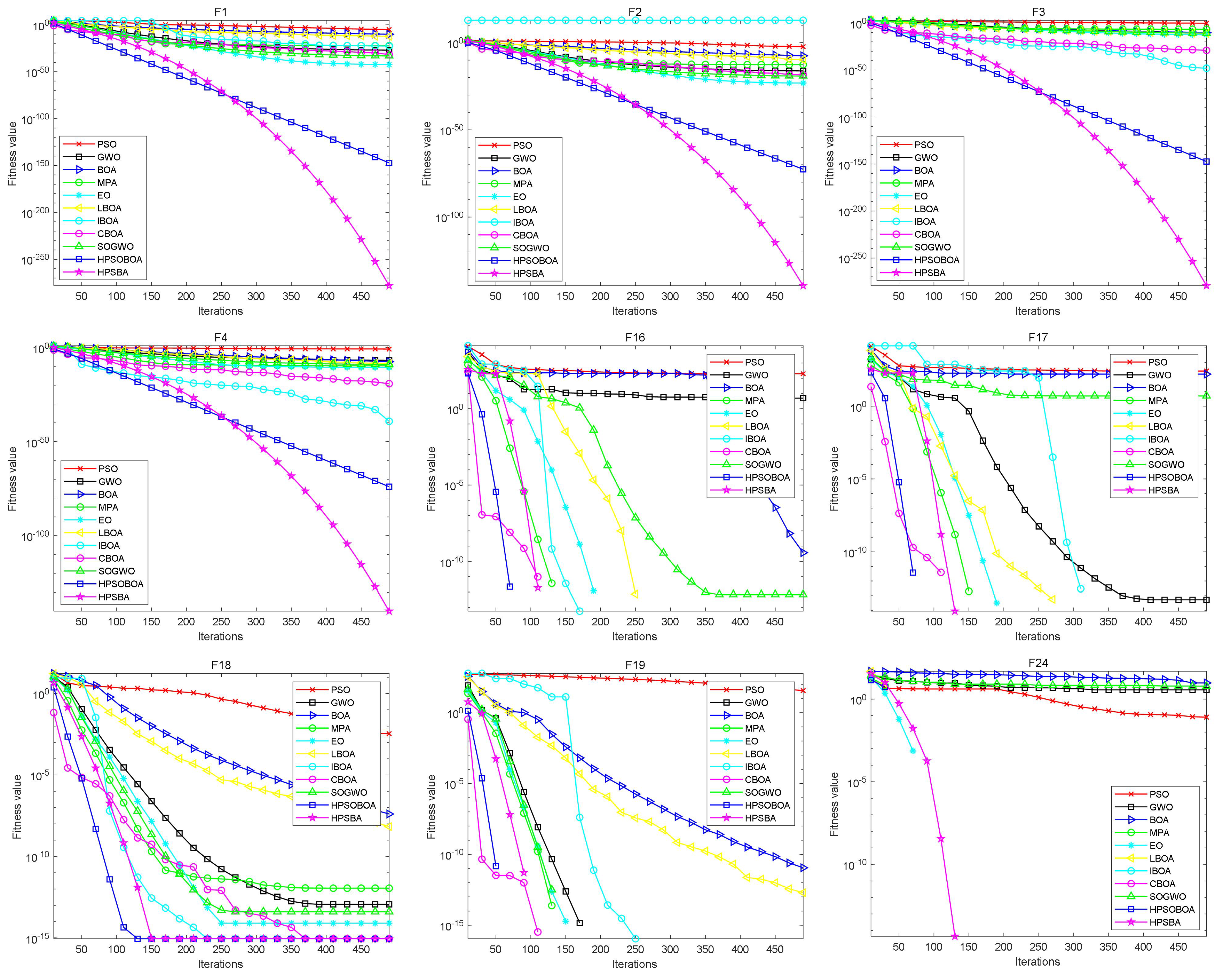
4.2.2. Convergence Behavior Analysis
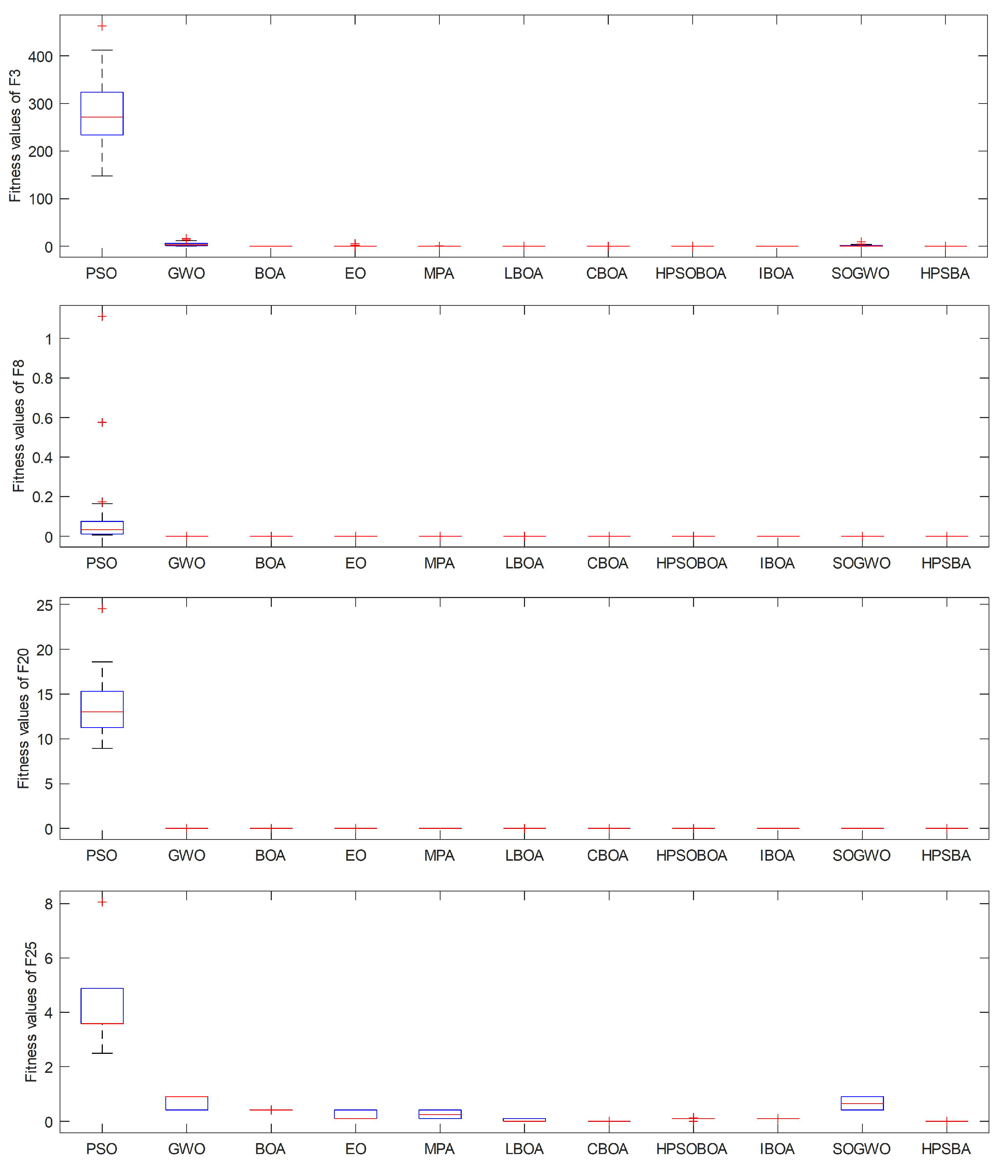
4.3. Comparison Results of HPSBA with Others (Dim = 100)
4.3.1. Analysis of the Numerical Results
4.3.2. Boxplot Results Analysis
5. Nodes Coverage Optimization in WSN
5.1. Parameter Setting and Pseudo Code of Node Coverage Using HPSBA
- PSO based node optimization coverage: Each target node runs the PSO to become a deployed node. Parameters that are considered for coverage are: inertial weight = 0.7, cognitive and social scaling parameters .
- BOA based node optimization coverage: Each target node runs the BOA to become a deployed node. Parameters that are considered for coverage are: probability switch weight , cognitive and social scaling parameters , and .
- MBOA based node optimization coverage: Each target node runs the MBOA to become a deployed node. Parameters that are considered for coverage are: probability switch weight , cognitive and social scaling parameters with chaotic adjust strategy, and .
- HPSBA based node optimization coverage: Each target node runs the proposed HPSBA to become a deployed node. Parameters that are considered for coverage are set as follows: initial value of inertial weight = 0.9, probability switch weight , cognitive and social scaling parameters and .
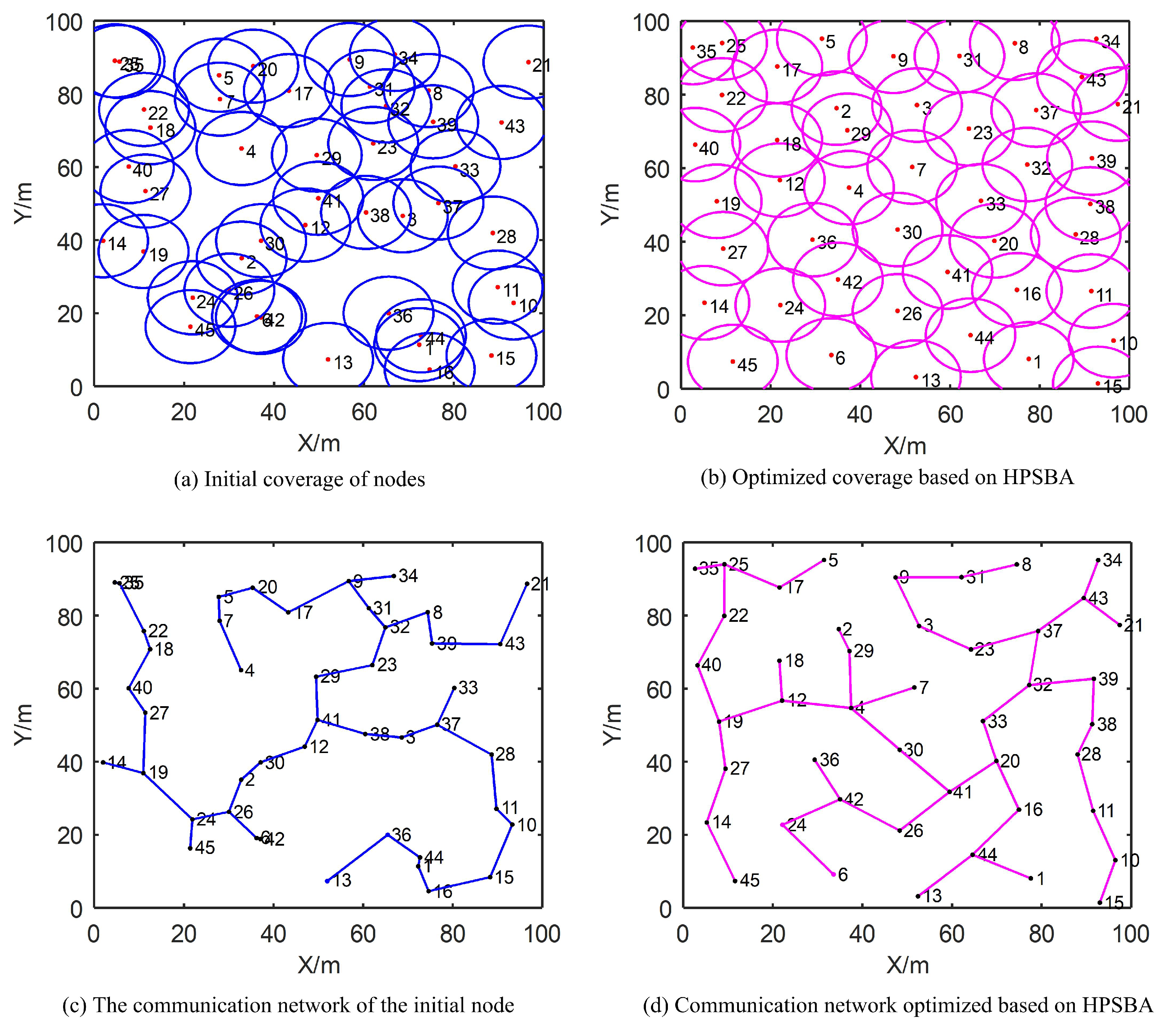
5.2. Results Analyses of Coverage Optimization Problem
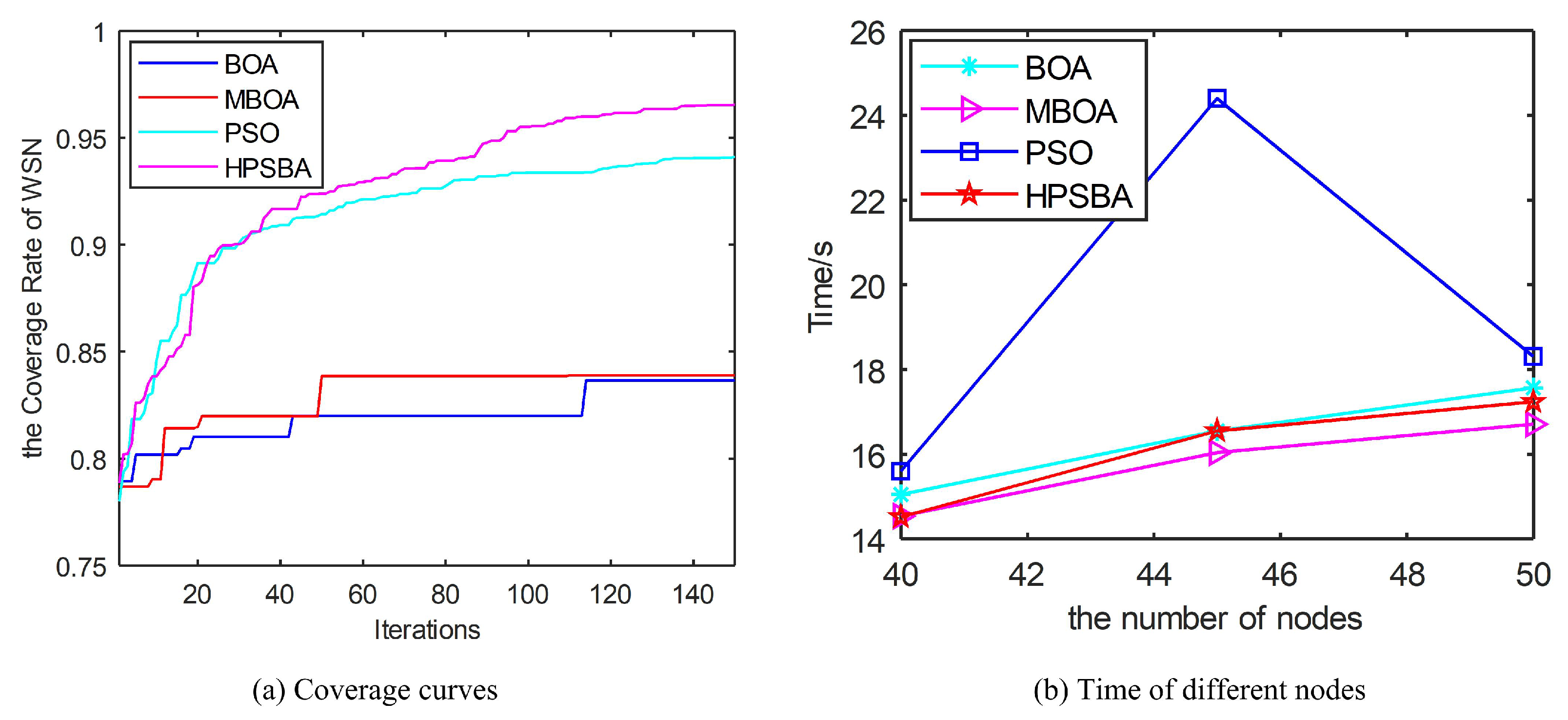
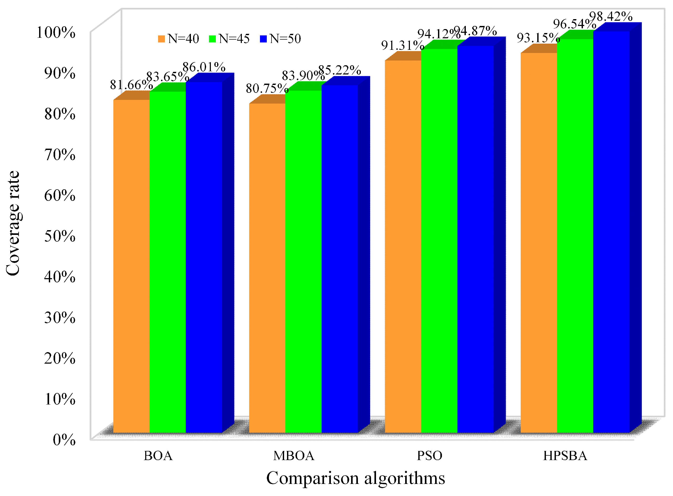
5.2.1. The Effect of the Number of Nodes on Coverage
5.2.2. The Effect of the Number of Iterations on Coverage
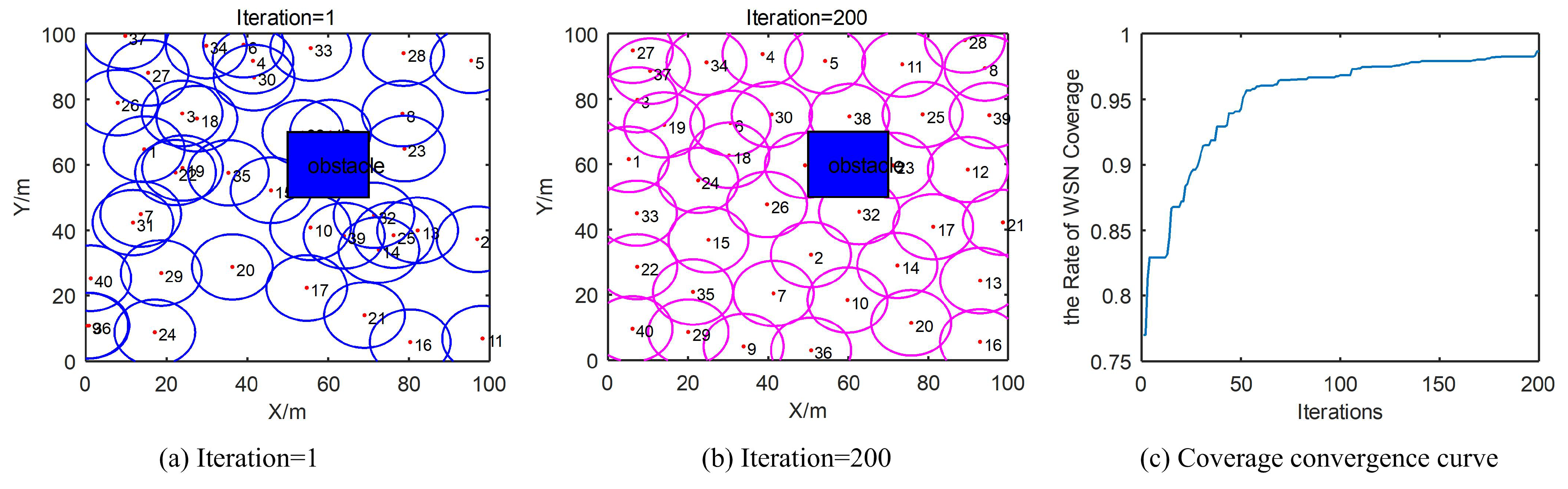
5.2.3. Node Obstacle Avoidance Coverage Based on HPSBA
6. Conclusions
Author Contributions
Funding
Institutional Review Board Statement
Informed Consent Statement
Data Availability Statement
Conflicts of Interest
References
- Kennedy, J.; Eberhart, R. Particle swarm optimization. In Proceedings of the ICNN’95-International Conference on Neural Networks, Perth, Australia, 27 November–1 December 1995; Volume 4, pp. 1942–1948. [Google Scholar]
- Gandomi, A.H.; Yang, X.S.; Alavi, A.H. Cuckoo search algorithm: A metaheuristic approach to solve structural optimization problems. Eng. Comput. 2013, 29, 17–35. [Google Scholar]
- Mirjalili, S.; Mirjalili, S.M.; Lewis, A. Grey wolf optimizer. Adv. Eng. Softw. 2014, 69, 46–61. [Google Scholar]
- Mirjalili, S.; Lewis, A. The whale optimization algorithm. Adv. Eng. Softw. 2016, 95, 51–67. [Google Scholar]
- Faramarzi, A.; Heidarinejad, M.; Mirjalili, S.; Gandomi, A.H. Marine Predators Algorithm: A nature-inspired metaheuristic. Expert Syst. Appl. 2020, 152, 113377. [Google Scholar]
- Dorigo, M.; Di Caro, G. Ant colony optimization: A new meta-heuristic. In Proceedings of the 1999 Congress on Evolutionary Computation-CEC99 (Cat. No. 99TH8406), Washington, DC, USA, 6–9 July 1999; Volume 2, pp. 1470–1477. [Google Scholar]
- Yang, X.S. Nature-Inspired Metaheuristic Algorithms; Luniver Press: Frome, UK, 2010. [Google Scholar]
- Mirjalili, S. Moth-flame optimization algorithm: A novel nature-inspired heuristic paradigm. Knowl.-Based Syst. 2015, 89, 228–249. [Google Scholar]
- Saremi, S.; Mirjalili, S.; Lewis, A. Grasshopper optimisation algorithm: Theory and application. Adv. Eng. Softw. 2017, 105, 30–47. [Google Scholar]
- Arora, S.; Singh, S. Butterfly optimization algorithm: A novel approach for global optimization. Soft Comput. 2019, 23, 715–734. [Google Scholar]
- Holland, J.H. Genetic algorithms. Sci. Am. 1992, 267, 66–73. [Google Scholar]
- Storn, R.; Price, K. Differential evolution—A simple and efficient heuristic for global optimization over continuous spaces. J. Glob. Optim. 1997, 11, 341–359. [Google Scholar]
- Simon, D. Biogeography-based optimization. IEEE Trans. Evol. Comput. 2008, 12, 702–713. [Google Scholar]
- Koza, J.R. Genetic programming II: Automatic discovery of reusable subprograms. Cambridge MA USA 1994, 13, 32. [Google Scholar]
- Kirkpatrick, S.; Gelatt, C.D., Jr.; Vecchi, M.P. Optimization by simulated annealing. Science 1983, 220, 671–680. [Google Scholar]
- Rashedi, E.; Nezamabadi-pour, H.; Saryazdi, S. GSA: A Gravitational Search Algorithm. Inf. Sci. 2009, 179, 2232–2248. [Google Scholar] [CrossRef]
- Geem, Z.W.; Kim, J.H.; Loganathan, G.V. A new heuristic optimization algorithm: Harmony search. Simulation 2001, 76, 60–68. [Google Scholar]
- Mirjalili, S. SCA: A sine cosine algorithm for solving optimization problems. Knowl.-Based Syst. 2016, 96, 120–133. [Google Scholar]
- Faramarzi, A.; Heidarinejad, M.; Stephens, B.; Mirjalili, S. Equilibrium optimizer: A novel optimization algorithm. Knowl.-Based Syst. 2020, 191, 105190. [Google Scholar]
- Ahmadianfar, I.; Bozorg-Haddad, O.; Chu, X. Gradient-based optimizer: A new metaheuristic optimization algorithm. Inf. Sci. 2020, 540, 131–159. [Google Scholar]
- Rao, R.V.; Savsani, V.J.; Vakharia, D. Teaching–learning-based optimization: An optimization method for continuous non-linear large scale problems. Inf. Sci. 2012, 183, 1–15. [Google Scholar]
- Glover, F. Tabu search: A tutorial. Interfaces 1990, 20, 74–94. [Google Scholar]
- Kumar, M.; Kulkarni, A.J.; Satapathy, S.C. Socio evolution & learning optimization algorithm: A socio-inspired optimization methodology. Future Gener. Comput. Syst. 2018, 81, 252–272. [Google Scholar]
- Askari, Q.; Younas, I.; Saeed, M. Political Optimizer: A novel socio-inspired meta-heuristic for global optimization. Knowl.-Based Syst. 2020, 195, 105709. [Google Scholar]
- Tu, J.; Chen, H.; Wang, M.; Gandomi, A.H. The colony predation algorithm. J. Bionic Eng. 2021, 18, 674–710. [Google Scholar]
- Li, C.; Chen, G.; Liang, G.; Luo, F.; Zhao, J.; Dong, Z.Y. Integrated optimization algorithm: A metaheuristic approach for complicated optimization. Inf. Sci. 2022, 586, 424–449. [Google Scholar]
- Yang, X.S. Flower pollination algorithm for global optimization. In International Conference on Unconventional Computing and Natural Computation; Springer: Berlin/Heidelberg, Germany, 2012; pp. 240–249. [Google Scholar]
- Kiran, M.S. TSA: Tree-seed algorithm for continuous optimization. Expert Syst. Appl. 2015, 42, 6686–6698. [Google Scholar]
- Liu, H.; Cai, Z.; Wang, Y. Hybridizing particle swarm optimization with differential evolution for constrained numerical and engineering optimization. Appl. Soft Comput. 2010, 10, 629–640. [Google Scholar]
- Razmjooy, N.; Ramezani, M. Training wavelet neural networks using hybrid particle swarm optimization and gravitational search algorithm for system identification. Int. J. Mechatronics, Electr. Comput. Technol. 2016, 6, 2987–2997. [Google Scholar]
- Garg, H. A hybrid GSA-GA algorithm for constrained optimization problems. Inf. Sci. 2019, 478, 499–523. [Google Scholar]
- Gong, Y.J.; Li, J.J.; Zhou, Y.; Li, Y.; Chung, H.S.H.; Shi, Y.H.; Zhang, J. Genetic learning particle swarm optimization. IEEE Trans. Cybern. 2015, 46, 2277–2290. [Google Scholar]
- El Sehiemy, R.A.; Selim, F.; Bentouati, B.; Abido, M. A novel multi-objective hybrid particle swarm and salp optimization algorithm for technical-economical-environmental operation in power systems. Energy 2020, 193, 116817. [Google Scholar]
- Arora, S.; Singh, S. Node localization in wireless sensor networks using butterfly optimization algorithm. Arab. J. Sci. Eng. 2017, 42, 3325–3335. [Google Scholar]
- Tan, L.S.; Zainuddin, Z.; Ong, P. Wavelet neural networks based solutions for elliptic partial differential equations with improved butterfly optimization algorithm training. Appl. Soft Comput. 2020, 95, 106518. [Google Scholar]
- Zhi, Y.; Weiqing, W.; Haiyun, W.; Khodaei, H. Improved butterfly optimization algorithm for CCHP driven by PEMFC. Appl. Therm. Eng. 2020, 173, 114766. [Google Scholar]
- Shams, I.; Mekhilef, S.; Tey, K.S. Maximum power point tracking using modified butterfly optimization algorithm for partial shading, uniform shading, and fast varying load conditions. IEEE Trans. Power Electron. 2020, 36, 5569–5581. [Google Scholar]
- Mengjian, Z.; Daoyin, L.; Qin, T.; Jing, Y. A Chaotic Hybrid Butterfly Optimization Algorithm with Particle Swarm Optimization for High-Dimensional Optimization Problems. Symmetry 2020, 12, 1800. [Google Scholar] [CrossRef]
- Akyildiz, I.F.; Su, W.; Sankarasubramaniam, Y.; Cayirci, E. Wireless sensor networks: A survey. Comput. Netw. 2002, 38, 393–422. [Google Scholar]
- Rashid, B.; Rehmani, M.H. Applications of wireless sensor networks for urban areas: A survey. J. Netw. Comput. Appl. 2016, 60, 192–219. [Google Scholar]
- Liao, W.H.; Kao, Y.; Wu, R.T. Ant colony optimization based sensor deployment protocol for wireless sensor networks. Expert Syst. Appl. 2011, 38, 6599–6605. [Google Scholar]
- Adulyasas, A.; Sun, Z.; Wang, N. Connected Coverage Optimization for Sensor Scheduling in Wireless Sensor Networks. IEEE Sensors J. 2015, 15, 3877–3892. [Google Scholar] [CrossRef]
- Wang, X.; Zhang, H.; Fan, S.; Gu, H. Coverage Control of Sensor Networks in IoT Based on RPSO. IEEE Internet Things J. 2018, 5, 3521–3532. [Google Scholar] [CrossRef]
- Yang, M.; Wang, A.; Sun, G.; Zhang, Y. Deploying charging nodes in wireless rechargeable sensor networks based on improved firefly algorithm. Comput. Electr. Eng. 2018, 72, 719–731. [Google Scholar] [CrossRef]
- Miao, Z.; Yuan, X.; Zhou, F.; Qiu, X.; Song, Y.; Chen, K. Grey wolf optimizer with an enhanced hierarchy and its application to the wireless sensor network coverage optimization problem. Appl. Soft Comput. 2020, 96, 106602. [Google Scholar] [CrossRef]
- Wang, S.; You, H.; Yue, Y.; Cao, L. A novel topology optimization of coverage-oriented strategy for wireless sensor networks. Int. J. Distrib. Sens. Netw. 2021, 17, 1550147721992298. [Google Scholar] [CrossRef]
- Dao, T.K.; Chu, S.C.; Nguyen, T.T.; Nguyen, T.D.; Nguyen, V.T. An Optimal WSN Node Coverage Based on Enhanced Archimedes Optimization Algorithm. Entropy 2022, 24, 1018. [Google Scholar] [CrossRef]
- Abdollahzadeh, S.; Navimipour, N.J. Deployment strategies in the wireless sensor network: A comprehensive review. Comput. Commun. 2016, 91–92, 1–16. [Google Scholar] [CrossRef]
- Zhang, M.; Yang, J.; Qin, T. An Adaptive Three-Dimensional Improved Virtual Force Coverage Algorithm for Nodes in WSN. Axioms 2022, 11, 199. [Google Scholar] [CrossRef]
- Zhang, M.; Wang, D.; Yang, J. Hybrid-Flash Butterfly Optimization Algorithm with Logistic Mapping for Solving the Engineering Constrained Optimization Problems. Entropy 2022, 24, 525. [Google Scholar] [CrossRef]
- May, R.M. Simple mathematical models with very complicated dynamics. Nature 1976, 261, 459–467. [Google Scholar] [CrossRef]
- Solis, F.J.; Wets, R.J.B. Minimization by random search techniques. Math. Oper. Res. 1981, 6, 19–30. [Google Scholar] [CrossRef]
- Zhang, M.-J.; Long, D.-Y.; Wang, X.; Yang, J. Research on Convergence of Grey Wolf Optimization Algorithm Based on Markov Chain. Acta Electron. Sin. 2020, 48, 1587–1595. [Google Scholar] [CrossRef]
- Dhargupta, S.; Ghosh, M.; Mirjalili, S.; Sarkar, R. Selective Opposition based Grey Wolf Optimization. Expert Syst. Appl. 2020, 151, 113389. [Google Scholar] [CrossRef]
- Knowles, J.; Corne, D. A new evolutionary approach to the degree-constrained minimum spanning tree problem. IEEE Trans. Evol. Comput. 2000, 4, 125–134. [Google Scholar] [CrossRef]
- LaTorre, A.; Molina, D.; Osaba, E.; Poyatos, J.; Del Ser, J.; Herrera, F. A prescription of methodological guidelines for comparing bio-inspired optimization algorithms. Swarm Evol. Comput. 2021, 67, 100973. [Google Scholar]


| c(0) | Schwefel 1.2 | Solomon | ||||
|---|---|---|---|---|---|---|
| Mean | Std | Time/s | Mean | Std | Time/s | |
| 0.15 | 5.28E-299 | 0 | 1.15 | 3.85E-301 | 0 | 0.17 |
| 0.25 | 4.75E-300 | 0 | 1.11 | 1.49E-223 | 0 | 0.17 |
| 0.35 | 7.70E-300 | 0 | 1.12 | 5.73E-301 | 0 | 0.17 |
| 0.45 | 3.49E-299 | 0 | 1.11 | 1.87E-301 | 0 | 0.17 |
| 0.55 | 4.54E-299 | 0 | 1.13 | 2.40E-301 | 0 | 0.17 |
| 0.65 | 3.16E-299 | 0 | 1.11 | 8.90E-301 | 0 | 0.17 |
| 0.75 | 7.87E-298 | 0 | 1.11 | 9.75E-222 | 0 | 0.17 |
| 0.85 | 4.82E-299 | 0 | 1.12 | 4.40E-301 | 0 | 0.17 |
| 0.95 | 3.16E-299 | 0 | 1.12 | 1.93E-301 | 0 | 0.17 |
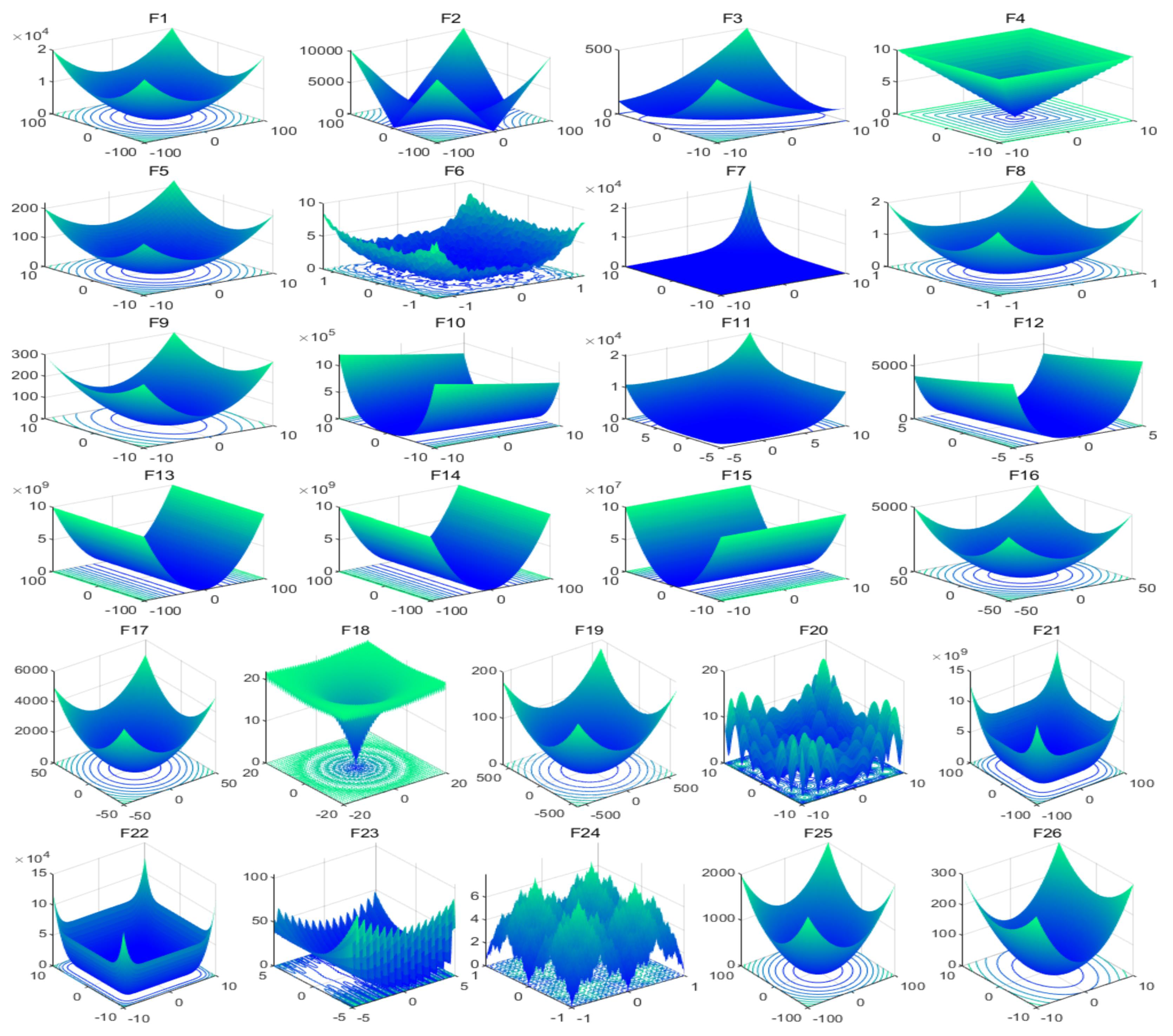
| Name | Formula | Search Range | Dim | Category | |
|---|---|---|---|---|---|
| Sphere | [−100,100] | 30/100 | 0 | U | |
| Schwefel 2.22 | [−10,10] | 30/100 | 0 | U | |
| Schwefel 1.2 | [−10,10] | 30/100 | 0 | U | |
| Schwefel 2.21 | [−10,10] | 30/100 | 0 | U | |
| Step | [−10,10] | 30/100 | 0 | U | |
| Quartic | [−1.28,1.28] | 30/100 | 0 | U | |
| Exponential | [−10,10] | 30/100 | 0 | U | |
| Sum Power | [−1,1] | 30/100 | 0 | U | |
| Sum Square | [−10,10] | 30/100 | 0 | U | |
| Rosenbrock | [−10,10] | 30/100 | 0 | U | |
| Zakharov | [−5.12,5.12] | 30/100 | 0 | U | |
| Trid | [−5,5] | 30/100 | 0 | U | |
| Elliptic | [−100,100] | 30/100 | 0 | U | |
| Cigar | [−100,100] | 30/100 | 0 | U | |
| Tablet | [−10,10] | 30/100 | 0 | U | |
| Rastrigin | [−5.12,5.12] | 30/100 | 0 | M | |
| NCRastrigin | [−5.12,5.12] | 30/100 | 0 | M | |
| Ackley | [−20,20] | 30/100 | 0 | M | |
| Griewank | [−600,600] | 30/100 | 0 | M | |
| Alpine | [−10,10] | 30/100 | 0 | M | |
| Penalized 1 | [−10,10] | 30/100 | 0 | M | |
| Penalized 2 | [−5,5] | 30/100 | 0 | M | |
| Levy | [−2,2] | 30/100 | 0 | M | |
| Weierstrass | [−1,1] | 30/100 | 0 | M | |
| Solomon | [−20,20] | 30/100 | 0 | M | |
| Bohachevsky | [−5,5] | 30/100 | 0 | M |
| Algorithms | Parameter Settings |
|---|---|
| PSO | |
| GWO | |
| BOA | |
| EO | |
| MPA | |
| LBOA | |
| CBOA | |
| HPSOBOA | |
| IBOA | |
| SOGWO | |
| HPSBA |
| Functions | PSO | GWO | BOA | EO | MPA | LBOA | CBOA | HPSOBOA | IBOA | SOGWO | HPSBA | |
|---|---|---|---|---|---|---|---|---|---|---|---|---|
| F1 | Mean | 1.16E-01 | 1.87E-27 | 7.70E-11 | 3.35E-40 | 5.72E-23 | 3.54E-12 | 2.20E-30 | 3.59E-152 | 7.47E-15 | 3.46E-33 | 3.29E-252 |
| Std | 3.89E-02 | 3.11E-27 | 6.78E-12 | 1.70E-39 | 5.83E-23 | 3.57E-12 | 4.29E-30 | 7.89E-153 | 1.72E-15 | 7.28E-33 | 0.00E+00 | |
| F2 | Mean | 6.35E-01 | 9.50E-17 | 2.35E-08 | 6.78E-24 | 2.53E-13 | 1.24E-09 | 3.92E-19 | 5.04E-60 | 4.97E+12 | 8.25E-20 | 2.52E-134 |
| Std | 2.05E-01 | 7.46E-17 | 6.49E-09 | 6.18E-24 | 2.68E-13 | 2.10E-09 | 6.67E-19 | 2.06E-59 | 1.22E+13 | 9.41E-20 | 6.87E-134 | |
| F3 | Mean | 4.16E+00 | 7.10E-08 | 5.31E-11 | 2.38E-11 | 2.71E-06 | 2.77E-12 | 1.11E-30 | 4.05E-153 | 9.32E-15 | 1.97E-09 | 7.60E-300 |
| Std | 9.64E-01 | 1.69E-07 | 5.83E-12 | 1.04E-10 | 7.11E-06 | 2.71E-12 | 3.47E-30 | 1.13E-153 | 1.11E-15 | 8.79E-09 | 0.00E+00 | |
| F4 | Mean | 3.36E-01 | 7.05E-08 | 2.65E-08 | 2.10E-11 | 3.39E-10 | 2.48E-09 | 1.48E-19 | 1.05E-77 | 8.05E-12 | 1.82E-09 | 6.02E-152 |
| Std | 4.82E-02 | 4.84E-08 | 2.94E-09 | 4.31E-11 | 2.12E-10 | 3.13E-09 | 2.49E-19 | 7.23E-79 | 1.06E-12 | 1.47E-09 | 1.69E-152 | |
| F5 | Mean | 7.12E-02 | 5.40E-01 | 5.23E+00 | 7.61E-06 | 3.42E-08 | 3.40E+00 | 4.55E+00 | 4.12E-02 | 3.36E+00 | 3.46E-01 | 5.38E+00 |
| Std | 3.20E-02 | 3.28E-01 | 6.84E-01 | 6.22E-06 | 1.73E-08 | 6.50E-01 | 5.83E-01 | 2.40E-02 | 7.86E-01 | 2.66E-01 | 6.36E-01 | |
| F6 | Mean | 2.60E-01 | 1.79E-03 | 1.99E-03 | 1.36E-03 | 1.28E-03 | 1.92E-03 | 1.17E-04 | 2.31E-04 | 3.10E-04 | 1.20E-03 | 9.21E-05 |
| Std | 8.64E-02 | 9.30E-04 | 5.51E-04 | 9.12E-04 | 7.43E-04 | 9.45E-04 | 1.17E-04 | 3.77E-04 | 2.58E-04 | 5.60E-04 | 9.73E-05 | |
| F7 | Mean | 0.00E+00 | 3.19E-58 | 4.94E-11 | 7.18E-66 | 7.18E-66 | 6.36E-21 | 3.84E-19 | 1.53E-62 | 7.09E-14 | 8.16E-61 | 8.51E-16 |
| Std | 0.00E+00 | 1.20E-57 | 1.34E-10 | 1.02E-78 | 1.40E-69 | 2.34E-20 | 1.16E-18 | 6.12E-63 | 3.06E-13 | 4.36E-60 | 4.27E-15 | |
| F8 | Mean | 7.23E-07 | 1.75E-95 | 8.88E-14 | 1.97E-134 | 1.98E-60 | 8.27E-16 | 1.46E-36 | 1.02E-156 | 4.45E-19 | 2.00E-116 | 1.70E-307 |
| Std | 1.17E-06 | 9.25E-95 | 5.52E-14 | 9.42E-134 | 4.89E-60 | 9.08E-16 | 6.48E-36 | 8.09E-158 | 2.44E-19 | 9.70E-116 | 0.00E+00 | |
| F9 | Mean | 7.51E-01 | 2.35E-28 | 6.94E-11 | 1.36E-41 | 4.83E-24 | 3.11E-12 | 8.60E-31 | 2.02E-152 | 9.61E-15 | 2.03E-34 | 3.19E-263 |
| Std | 2.87E-01 | 4.02E-28 | 8.22E-12 | 3.56E-41 | 6.23E-24 | 4.11E-12 | 1.77E-30 | 2.89E-153 | 1.34E-15 | 2.28E-34 | 0.00E+00 | |
| F10 | Mean | 5.99E+01 | 2.72E+01 | 2.89E+01 | 2.53E+01 | 2.51E+01 | 2.88E+01 | 2.89E+01 | 2.71E+01 | 2.89E+01 | 2.68E+01 | 2.89E+01 |
| Std | 3.87E+01 | 8.55E-01 | 2.70E-02 | 1.54E-01 | 3.89E-01 | 3.25E-02 | 3.73E-02 | 6.30E+00 | 3.53E-02 | 8.00E-01 | 3.37E-02 | |
| F11 | Mean | 1.47E+00 | 3.17E-28 | 6.67E-11 | 3.42E-41 | 1.23E-23 | 3.52E-12 | 2.81E-30 | 6.89E-153 | 8.32E-15 | 1.18E-33 | 1.28E-252 |
| Std | 8.03E-01 | 5.15E-28 | 7.26E-12 | 1.26E-40 | 2.24E-23 | 3.22E-12 | 7.66E-30 | 1.17E-153 | 1.52E-15 | 2.59E-33 | 0.00E+00 | |
| F12 | Mean | 4.22E+00 | 6.67E-01 | 9.74E-01 | 6.67E-01 | 6.67E-01 | 9.18E-01 | 9.76E-01 | 1.00E+00 | 9.35E-01 | 6.67E-01 | 6.67E-01 |
| Std | 1.82E+00 | 3.76E-05 | 8.43E-03 | 3.08E-10 | 3.87E-08 | 2.48E-02 | 9.00E-03 | 1.25E-05 | 1.81E-02 | 4.37E-06 | 1.86E-04 | |
| F13 | Mean | 6.08E-31 | 0.00E+00 | 2.80E-21 | 0.00E+00 | 3.55E-174 | 5.49E-26 | 1.77E-34 | 2.30E-148 | 8.87E-31 | 0.00E+00 | 2.44E-302 |
| Std | 2.42E-30 | 0.00E+00 | 8.91E-21 | 0.00E+00 | 0.00E+00 | 1.14E-25 | 5.23E-34 | 1.14E-147 | 4.33E-30 | 0.00E+00 | 0.00E+00 | |
| F14 | Mean | 1.16E-24 | 2.82E-205 | 1.92E-17 | 7.30E-207 | 1.34E-61 | 3.31E-18 | 3.49E-31 | 1.95E-147 | 5.73E-23 | 4.59E-228 | 6.12E-296 |
| Std | 2.26E-24 | 0.00E+00 | 2.08E-17 | 0.00E+00 | 7.35E-61 | 4.01E-18 | 7.94E-31 | 4.53E-147 | 1.22E-22 | 0.00E+00 | 0.00E+00 | |
| F15 | Mean | 3.02E-30 | 6.90E-261 | 4.54E-19 | 8.38E-255 | 8.23E-94 | 1.65E-19 | 1.09E-34 | 1.92E-153 | 3.69E-22 | 1.06E-313 | 3.61E-304 |
| Std | 1.65E-29 | 0.00E+00 | 8.61E-19 | 0.00E+00 | 3.33E-93 | 3.98E-19 | 5.42E-34 | 6.79E-153 | 7.04E-22 | 0.00E+00 | 0.00E+00 | |
| F16 | Mean | 2.37E+02 | 4.02E+00 | 6.54E+01 | 1.89E-15 | 0.00E+00 | 0.00E+00 | 0.00E+00 | 0.00E+00 | 0.00E+00 | 2.27E+00 | 0.00E+00 |
| Std | 5.65E+01 | 3.88E+00 | 9.09E+01 | 1.04E-14 | 0.00E+00 | 0.00E+00 | 0.00E+00 | 0.00E+00 | 0.00E+00 | 3.20E+00 | 0.00E+00 | |
| F17 | Mean | 2.76E+02 | 8.31E+00 | 1.24E+02 | 2.33E-01 | 3.96E-07 | 0.00E+00 | 0.00E+00 | 0.00E+00 | 0.00E+00 | 8.87E+00 | 0.00E+00 |
| Std | 7.80E+01 | 4.39E+00 | 7.02E+01 | 6.26E-01 | 2.17E-06 | 0.00E+00 | 0.00E+00 | 0.00E+00 | 0.00E+00 | 5.03E+00 | 0.00E+00 | |
| F18 | Mean | 2.47E-01 | 9.05E-14 | 2.75E-08 | 8.47E-15 | 8.53E-13 | 2.47E-09 | 8.88E-16 | 8.88E-16 | 7.10E-12 | 4.14E-14 | 8.88E-16 |
| Std | 7.83E-02 | 1.67E-14 | 2.47E-09 | 1.80E-15 | 5.41E-13 | 1.38E-09 | 0.00E+00 | 0.00E+00 | 7.10E-13 | 2.89E-15 | 0.00E+00 | |
| F19 | Mean | 3.41E+01 | 3.23E-03 | 9.73E-12 | 0.00E+00 | 0.00E+00 | 1.79E-13 | 0.00E+00 | 0.00E+00 | 4.18E-16 | 2.70E-03 | 0.00E+00 |
| Std | 5.57E+00 | 8.81E-03 | 1.06E-11 | 0.00E+00 | 0.00E+00 | 3.96E-13 | 0.00E+00 | 0.00E+00 | 1.90E-15 | 5.90E-03 | 0.00E+00 | |
| F20 | Mean | 1.53E-01 | 4.74E-04 | 3.47E-09 | 6.29E-09 | 6.61E-14 | 6.42E-14 | 1.00E-19 | 9.42E-60 | 6.67E-12 | 3.52E-04 | 7.05E-136 |
| Std | 9.79E-02 | 7.66E-04 | 7.60E-09 | 3.44E-08 | 4.58E-14 | 1.86E-13 | 1.28E-19 | 2.99E-59 | 7.69E-13 | 5.84E-04 | 3.83E-135 | |
| F21 | Mean | 7.09E+00 | 5.03E-02 | 5.39E-01 | 3.46E-03 | 7.59E-05 | 2.90E-01 | 4.78E-01 | 2.47E-03 | 1.48E+00 | 3.38E-02 | 5.49E-01 |
| Std | 3.04E+00 | 2.12E-02 | 1.58E-01 | 1.89E-02 | 4.15E-04 | 9.21E-02 | 1.36E-01 | 2.64E-03 | 2.31E-01 | 1.49E-02 | 1.37E-01 | |
| F22 | Mean | 8.06E-03 | 7.07E-01 | 3.40E+00 | 2.18E-02 | 3.45E-03 | 2.37E+00 | 3.00E+00 | 4.07E+00 | 2.63E+00 | 5.15E-01 | 3.42E+00 |
| Std | 4.77E-03 | 2.10E-01 | 4.83E-01 | 4.72E-02 | 1.65E-02 | 6.28E-01 | 5.74E-01 | 2.15E+00 | 5.90E-01 | 1.88E-01 | 5.79E-01 | |
| F23 | Mean | 3.88E-01 | 1.67E+00 | 1.18E+01 | 1.52E-01 | 1.38E-01 | 9.31E+00 | 1.01E+01 | 8.89E-01 | 1.06E+01 | 1.25E+00 | 1.09E+01 |
| Std | 2.43E-01 | 1.02E+00 | 2.10E+00 | 3.22E-01 | 1.89E-01 | 2.67E+00 | 2.71E+00 | 1.18E+00 | 1.94E+00 | 8.19E-01 | 3.23E+00 | |
| F24 | Mean | 5.70E+00 | 4.93E+00 | 1.23E+00 | 0.00E+00 | 0.00E+00 | 0.00E+00 | 0.00E+00 | 0.00E+00 | 0.00E+00 | 4.61E+00 | 0.00E+00 |
| Std | 2.76E+00 | 2.04E+00 | 2.35E+00 | 0.00E+00 | 0.00E+00 | 0.00E+00 | 0.00E+00 | 0.00E+00 | 0.00E+00 | 1.67E+00 | 0.00E+00 | |
| F25 | Mean | 7.11E-01 | 2.79E-01 | 7.66E-01 | 9.95E-02 | 9.95E-02 | 2.99E-02 | 1.68E-32 | 6.43E-02 | 9.95E-02 | 2.89E-01 | 4.07E-301 |
| Std | 3.41E-01 | 1.49E-01 | 2.18E-01 | 2.08E-12 | 7.05E-17 | 4.64E-02 | 3.64E-32 | 4.99E-02 | 1.24E-06 | 1.46E-01 | 0.00E+00 | |
| F26 | Mean | 1.24E+00 | 0.00E+00 | 8.02E-11 | 0.00E+00 | 0.00E+00 | 4.45E-12 | 0.00E+00 | 0.00E+00 | 9.79E-15 | 0.00E+00 | 0.00E+00 |
| Std | 5.92E-01 | 0.00E+00 | 8.59E-12 | 0.00E+00 | 0.00E+00 | 5.45E-12 | 0.00E+00 | 0.00E+00 | 1.33E-15 | 0.00E+00 | 0.00E+00 | |
| +/-/≈ | 1/25/0 | 0/24/2 | 0/26/0 | 1/20/5 | 4/18/4 | 0/23/3 | 0/20/6 | 0/20/6 | 0/23/3 | 1/22/3 | ∼ | |
| Rank | 7 | 6 | 8 | 3 | 2 | 4 | 3 | 3 | 5 | 4 | 1 | |
| Functions | PSO | GWO | BOA | EO | MPA | LBOA | CBOA | HPSOBOA | IBOA | SOGWO | HPSBA | |
|---|---|---|---|---|---|---|---|---|---|---|---|---|
| F1 | Mean | 8.45E+00 | 1.48E-12 | 8.75E-11 | 4.14E-29 | 1.77E-19 | 6.12E-12 | 6.86E-30 | 3.31E-152 | 9.05E-15 | 6.44E-15 | 7.12E-299 |
| Std | 7.28E-01 | 1.83E-12 | 9.69E-12 | 5.38E-29 | 2.10E-19 | 7.39E-12 | 1.51E-29 | 1.35E-152 | 1.87E-15 | 8.86E-15 | 0.00E+00 | |
| F2 | Mean | 1.82E+01 | 4.04E-08 | 4.71E+50 | 1.85E-17 | 1.43E-11 | 1.52E+50 | 3.74E-18 | 1.48E+36 | 8.10E+49 | 1.60E-09 | 4.35E+50 |
| Std | 2.23E+00 | 1.35E-08 | 1.92E+51 | 1.36E-17 | 1.15E-11 | 6.27E+50 | 6.73E-18 | 2.80E+35 | 3.95E+50 | 6.14E-10 | 1.42E+51 | |
| F3 | Mean | 2.80E+02 | 4.54E+00 | 6.08E-11 | 3.15E-01 | 1.04E-01 | 3.40E-12 | 4.42E-31 | 1.48E-152 | 9.74E-15 | 1.39E+00 | 1.06E-299 |
| Std | 7.38E+01 | 4.04E+00 | 5.91E-12 | 1.11E+00 | 1.50E-01 | 3.36E-12 | 8.91E-31 | 1.35E-152 | 1.11E-15 | 1.98E+00 | 0.00E+00 | |
| F4 | Mean | 1.77E+00 | 5.79E-02 | 2.98E-08 | 2.64E-01 | 2.40E-08 | 2.86E-09 | 1.20E-19 | 1.08E-77 | 8.47E-12 | 1.60E-02 | 7.43E-152 |
| Std | 1.71E-01 | 6.77E-02 | 2.71E-09 | 1.45E+00 | 1.16E-08 | 2.88E-09 | 1.58E-19 | 5.19E-79 | 1.17E-12 | 1.52E-02 | 2.49E-152 | |
| F5 | Mean | 5.47E+00 | 9.20E+00 | 2.21E+01 | 2.94E+00 | 2.56E+00 | 2.03E+01 | 2.12E+01 | 1.48E-01 | 2.07E+01 | 7.67E+00 | 2.24E+01 |
| Std | 9.43E-01 | 9.87E-01 | 1.06E+00 | 5.46E-01 | 7.71E-01 | 1.60E+00 | 1.18E+00 | 1.27E-01 | 1.06E+00 | 9.06E-01 | 8.81E-01 | |
| F6 | Mean | 6.02E+01 | 7.14E-03 | 2.11E-03 | 2.44E-03 | 1.87E-03 | 2.01E-03 | 1.03E-04 | 1.13E-04 | 2.77E-04 | 4.90E-03 | 6.85E-05 |
| Std | 1.38E+01 | 2.79E-03 | 8.96E-04 | 1.41E-03 | 9.55E-04 | 1.18E-03 | 7.42E-05 | 1.28E-04 | 2.49E-04 | 1.70E-03 | 6.09E-05 | |
| F7 | Mean | 0.00E+00 | 9.84E-135 | 1.71E-23 | 7.16E-218 | 1.70E-202 | 2.74E-28 | 4.05E-32 | 1.93E-207 | 1.92E-20 | 2.96E-155 | 4.15E-27 |
| Std | 0.00E+00 | 5.39E-134 | 8.68E-23 | 0.00E+00 | 0.00E+00 | 1.39E-27 | 1.12E-31 | 0.00E+00 | 8.47E-20 | 1.62E-154 | 2.27E-26 | |
| F8 | Mean | 9.97E-02 | 1.28E-66 | 7.32E-14 | 1.16E-129 | 2.23E-60 | 9.96E-16 | 4.86E-37 | 9.98E-157 | 4.00E-19 | 2.38E-64 | 1.82E-306 |
| Std | 2.20E-01 | 4.84E-66 | 6.04E-14 | 6.03E-129 | 4.85E-60 | 1.62E-15 | 1.49E-36 | 7.46E-158 | 2.59E-19 | 1.30E-63 | 0.00E+00 | |
| F9 | Mean | 2.82E+02 | 6.63E-13 | 8.60E-11 | 1.94E-29 | 8.17E-20 | 3.97E-12 | 1.13E-30 | 4.23E-152 | 9.06E-15 | 1.38E-15 | 4.72E-299 |
| Std | 5.17E+01 | 5.34E-13 | 8.92E-12 | 2.56E-29 | 5.83E-20 | 3.66E-12 | 2.60E-30 | 1.02E-152 | 1.95E-15 | 1.01E-15 | 0.00E+00 | |
| F10 | Mean | 1.24E+03 | 9.79E+01 | 9.89E+01 | 9.66E+01 | 9.69E+01 | 9.88E+01 | 9.89E+01 | 9.07E+01 | 9.89E+01 | 9.77E+01 | 9.89E+01 |
| Std | 2.28E+02 | 5.73E-01 | 2.93E-02 | 1.08E+00 | 8.66E-01 | 3.76E-02 | 4.76E-02 | 2.30E+01 | 3.48E-02 | 7.22E-01 | 3.49E-02 | |
| F11 | Mean | 3.65E+02 | 7.60E-13 | 8.13E-11 | 3.57E-29 | 3.77E-20 | 4.82E-12 | 3.26E-30 | 9.41E-153 | 1.00E-14 | 1.93E-15 | 4.59E-299 |
| Std | 7.04E+01 | 6.45E-13 | 6.27E-12 | 1.09E-28 | 3.04E-20 | 3.99E-12 | 1.45E-29 | 5.44E-153 | 1.66E-15 | 1.49E-15 | 0.00E+00 | |
| F12 | Mean | 6.01E+02 | 6.67E-01 | 9.98E-01 | 6.67E-01 | 6.67E-01 | 9.95E-01 | 9.98E-01 | 1.00E+00 | 9.96E-01 | 6.67E-01 | 9.99E-01 |
| Std | 1.55E+02 | 3.47E-05 | 8.04E-04 | 3.93E-08 | 1.41E-06 | 9.93E-04 | 5.10E-04 | 8.11E-05 | 8.74E-04 | 5.49E-06 | 4.19E-04 | |
| F13 | Mean | 1.06E-33 | 0.00E+00 | 5.13E-22 | 0.00E+00 | 3.61E-169 | 3.15E-25 | 3.19E-34 | 1.33E-150 | 4.62E-31 | 0.00E+00 | 1.53E-302 |
| Std | 5.50E-33 | 0.00E+00 | 1.69E-21 | 0.00E+00 | 0.00E+00 | 8.18E-25 | 1.63E-33 | 3.20E-150 | 1.56E-30 | 0.00E+00 | 0.00E+00 | |
| F14 | Mean | 6.38E-24 | 1.24E-205 | 3.84E-17 | 2.66E-201 | 1.86E-63 | 4.88E-18 | 3.01E-31 | 6.40E-150 | 9.63E-23 | 2.87E-186 | 3.05E-298 |
| Std | 1.76E-23 | 0.00E+00 | 6.24E-17 | 0.00E+00 | 1.02E-62 | 7.45E-18 | 6.15E-31 | 1.34E-149 | 2.26E-22 | 0.00E+00 | 0.00E+00 | |
| F15 | Mean | 1.88E-32 | 8.39E-261 | 1.23E-19 | 3.97E-253 | 9.63E-92 | 3.93E-19 | 1.55E-34 | 1.71E-153 | 3.26E-22 | 6.24E-310 | 1.69E-303 |
| Std | 5.59E-32 | 0.00E+00 | 2.55E-19 | 0.00E+00 | 4.94E-91 | 9.39E-19 | 8.12E-34 | 5.23E-153 | 4.34E-22 | 0.00E+00 | 0.00E+00 | |
| F16 | Mean | 4.87E+02 | 9.55E+00 | 1.77E-06 | 3.79E-15 | 0.00E+00 | 0.00E+00 | 0.00E+00 | 0.00E+00 | 0.00E+00 | 9.04E+00 | 0.00E+00 |
| Std | 6.30E+01 | 8.37E+00 | 9.70E-06 | 2.08E-14 | 0.00E+00 | 0.00E+00 | 0.00E+00 | 0.00E+00 | 0.00E+00 | 5.80E+00 | 0.00E+00 | |
| F17 | Mean | 4.34E+02 | 2.34E+01 | 7.57E+01 | 1.00E-01 | 0.00E+00 | 0.00E+00 | 0.00E+00 | 0.00E+00 | 5.92E-17 | 1.32E+01 | 0.00E+00 |
| Std | 6.22E+01 | 2.09E+01 | 2.31E+02 | 3.05E-01 | 0.00E+00 | 0.00E+00 | 0.00E+00 | 0.00E+00 | 3.24E-16 | 9.07E+00 | 0.00E+00 | |
| F18 | Mean | 2.52E+00 | 8.15E-08 | 3.08E-08 | 3.27E-14 | 2.87E-11 | 2.76E-09 | 8.88E-16 | 8.88E-16 | 7.78E-12 | 4.06E-09 | 8.88E-16 |
| Std | 1.91E-01 | 3.11E-08 | 2.55E-09 | 6.08E-15 | 1.33E-11 | 2.31E-09 | 0.00E+00 | 0.00E+00 | 9.15E-13 | 1.29E-09 | 0.00E+00 | |
| F19 | Mean | 1.38E+02 | 4.01E-03 | 6.69E-11 | 0.00E+00 | 0.00E+00 | 1.98E-12 | 0.00E+00 | 0.00E+00 | 9.25E-15 | 1.83E-03 | 0.00E+00 |
| Std | 1.42E+01 | 1.15E-02 | 2.72E-11 | 0.00E+00 | 0.00E+00 | 1.80E-12 | 0.00E+00 | 0.00E+00 | 4.81E-15 | 5.61E-03 | 0.00E+00 | |
| F20 | Mean | 1.33E+01 | 3.92E-03 | 2.01E-09 | 3.66E-18 | 3.01E-12 | 3.26E-11 | 1.05E-19 | 1.15E-57 | 7.60E-12 | 2.49E-03 | 1.27E-151 |
| Std | 3.35E+00 | 2.70E-03 | 1.85E-09 | 2.04E-18 | 2.42E-12 | 5.92E-11 | 1.32E-19 | 6.30E-57 | 9.27E-13 | 1.50E-03 | 3.56E-152 | |
| F21 | Mean | 1.13E-01 | 2.05E-01 | 9.83E-01 | 2.83E-02 | 3.74E-02 | 7.49E-01 | 9.33E-01 | 1.49E-03 | 7.70E-01 | 1.51E-01 | 1.09E+00 |
| Std | 8.19E-02 | 4.33E-02 | 8.89E-02 | 8.01E-03 | 9.89E-03 | 1.14E-01 | 1.20E-01 | 6.36E-04 | 1.10E-01 | 4.35E-02 | 7.82E-02 | |
| F22 | Mean | 1.02E+00 | 5.66E+00 | 9.99E+00 | 5.16E+00 | 6.05E+00 | 9.99E+00 | 9.98E+00 | 9.70E+00 | 9.94E+00 | 4.96E+00 | 9.99E+00 |
| Std | 1.98E-01 | 4.20E-01 | 5.25E-03 | 1.35E+00 | 2.96E+00 | 4.55E-03 | 4.85E-03 | 6.11E-01 | 1.34E-01 | 4.19E-01 | 2.48E-03 | |
| F23 | Mean | 2.35E+01 | 1.81E+01 | 6.84E+01 | 3.96E+00 | 4.54E+00 | 6.05E+01 | 6.85E+01 | 1.94E+00 | 6.54E+01 | 1.37E+01 | 6.69E+01 |
| Std | 7.20E+00 | 4.80E+00 | 4.20E+00 | 1.59E+00 | 1.69E+00 | 6.39E+00 | 4.94E+00 | 8.69E-01 | 5.49E+00 | 3.09E+00 | 5.65E+00 | |
| F24 | Mean | 5.16E+01 | 1.67E+01 | 2.66E+00 | 3.20E-05 | 0.00E+00 | 0.00E+00 | 0.00E+00 | 0.00E+00 | 0.00E+00 | 1.33E+01 | 0.00E+00 |
| Std | 9.49E+00 | 1.08E+01 | 3.18E+00 | 1.75E-04 | 0.00E+00 | 0.00E+00 | 0.00E+00 | 0.00E+00 | 0.00E+00 | 4.05E+00 | 0.00E+00 | |
| F25 | Mean | 3.97E+00 | 6.80E-01 | 4.00E-01 | 2.29E-01 | 2.49E-01 | 3.33E-02 | 1.09E-32 | 8.86E-02 | 9.95E-02 | 6.47E-01 | 7.39E-301 |
| Std | 1.06E+00 | 2.51E-01 | 3.16E-03 | 1.50E-01 | 1.52E-01 | 4.77E-02 | 3.81E-32 | 3.58E-02 | 3.00E-06 | 2.53E-01 | 0.00E+00 | |
| F26 | Mean | 6.60E+01 | 1.01E-13 | 8.60E-11 | 0.00E+00 | 0.00E+00 | 5.22E-12 | 0.00E+00 | 0.00E+00 | 7.87E-15 | 2.96E-16 | 0.00E+00 |
| Std | 6.71E+00 | 1.50E-13 | 8.49E-12 | 0.00E+00 | 0.00E+00 | 6.98E-12 | 0.00E+00 | 0.00E+00 | 1.50E-15 | 4.86E-16 | 0.00E+00 | |
| +/-/≈ | 1/25/0 | 1/25/0 | 0/26/0 | 2/21/3 | 0/21/5 | 0/23/3 | 1/19/6 | 4/16/6 | 0/24/2 | 1/25/0 | ∼ | |
| Rank | 7 | 7 | 8 | 4 | 4 | 5 | 3 | 2 | 6 | 7 | 1 | |
| Parameters | Setting Values | |
|---|---|---|
| Side length of coverage area/m | 100 × 100 | 100 × 100 |
| Number of nodes | 45 | 40, 45, 50 |
| Perception radius/m | 10 | 10 |
| Communication radius /m | 20 | 20 |
| Maximum iterations () | 100, 150, 200 | 150 |
| Boundary threshold/m | ||
| Item | = 100 | = 150 | = 200 | |||
|---|---|---|---|---|---|---|
| Cov/% | Time/s | Cov/% | Time/s | Cov/% | Time/s | |
| BOA | 84.79 | 12.21 | 83.65 | 16.55 | 86.42 | 40.98 |
| MBOA | 85.11 | 10.93 | 83.90 | 16.04 | 85.82 | 21.10 |
| PSO | 92.20 | 11.94 | 94.12 | 24.4 | 94.32 | 51.92 |
| HPSBA | 93.28 | 11.09 | 96.54 | 16.55 | 96.32 | 21.31 |
Publisher’s Note: MDPI stays neutral with regard to jurisdictional claims in published maps and institutional affiliations. |
© 2022 by the authors. Licensee MDPI, Basel, Switzerland. This article is an open access article distributed under the terms and conditions of the Creative Commons Attribution (CC BY) license (https://creativecommons.org/licenses/by/4.0/).
Share and Cite
Zhang, M.; Wang, D.; Yang, M.; Tan, W.; Yang, J. HPSBA: A Modified Hybrid Framework with Convergence Analysis for Solving Wireless Sensor Network Coverage Optimization Problem. Axioms 2022, 11, 675. https://doi.org/10.3390/axioms11120675
Zhang M, Wang D, Yang M, Tan W, Yang J. HPSBA: A Modified Hybrid Framework with Convergence Analysis for Solving Wireless Sensor Network Coverage Optimization Problem. Axioms. 2022; 11(12):675. https://doi.org/10.3390/axioms11120675
Chicago/Turabian StyleZhang, Mengjian, Deguang Wang, Ming Yang, Wei Tan, and Jing Yang. 2022. "HPSBA: A Modified Hybrid Framework with Convergence Analysis for Solving Wireless Sensor Network Coverage Optimization Problem" Axioms 11, no. 12: 675. https://doi.org/10.3390/axioms11120675