
A Novel Approach for the Approximate Solution of Wave Problems in Multi-Dimensional Orders with Computational Applications


Abstract
:1. Introduction
2. Preliminary Definitions of IT
3. Formulation of HITM
4. Convergence Analysis
- (1)
- ;
- (2)
- is forever in the neighborhood of meaning
- (3)
- .
- (1)
- Consider condition (1) by recognition of n such that , and the Banach fixed point theorem states that X has a fixed point (i.e., ). Therefore, we havewhere X is a nonlinear mapping. By considering that is an induction hypothesis, then
- (2)
- Our initial challenge is to demonstrate , which is attained by replacing m. Thus, for with as an initial condition. Consider that for is an induction theory. Thus, we haveNow, ∀, using (1), we obtain
- (3)
- Using condition (2) and , it follows that , and henceThus, converges.
5. Computational Applications
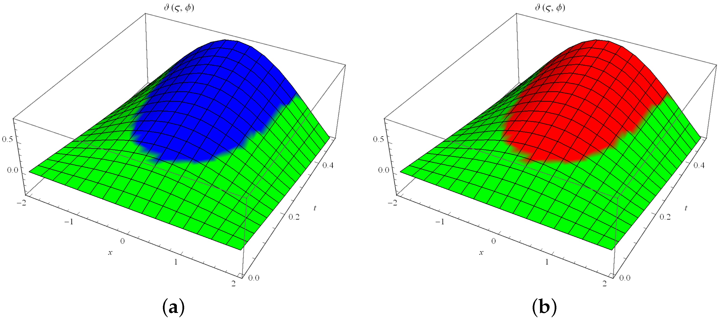
5.1. Example 1
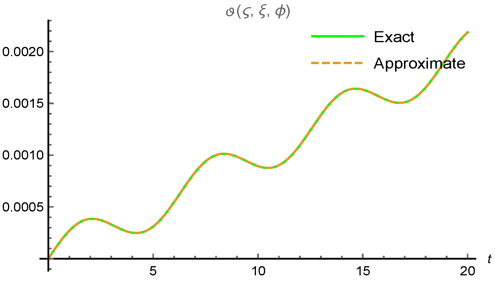
5.2. Example 2
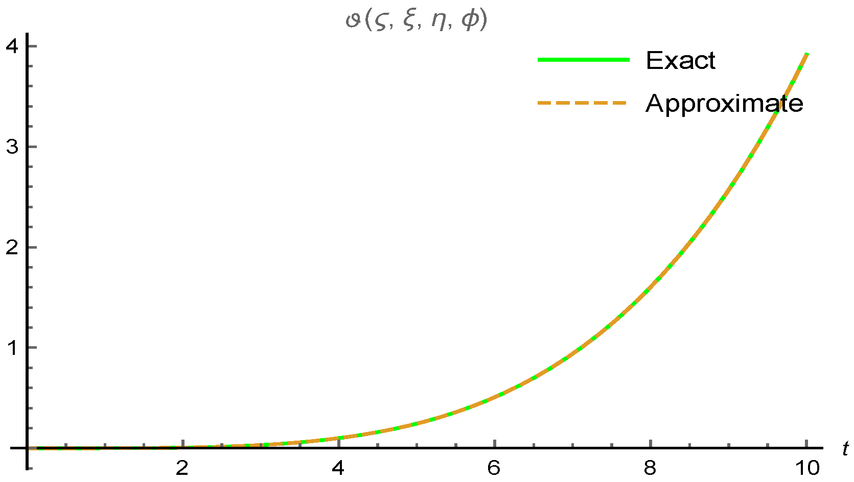
5.3. Example 3
6. Conclusions
Author Contributions
Funding
Institutional Review Board Statement
Informed Consent Statement
Data Availability Statement
Acknowledgments
Conflicts of Interest
References
- Liu, M.Z.; Cao, X.Q.; Zhu, X.Q.; Liu, B.N.; Peng, K.C. Variational Principles and Solitary Wave Solutions of Generalized Nonlinear Schrödinger Equation in the Ocean. J. Appl. Comput. Mech. 2021, 7, 1639–1648. [Google Scholar]
- Cakmak, M.; Alkan, S. A numerical method for solving a class of systems of nonlinear Pantograph differential equations. Alex. Eng. J. 2022, 61, 2651–2661. [Google Scholar] [CrossRef]
- Momani, S.; Odibat, Z. Analytical approach to linear fractional partial differential equations arising in fluid mechanics. Phys. Lett. A 2006, 355, 271–279. [Google Scholar] [CrossRef]
- Dehghan, M.; Manafian, J.; Saadatmandi, A. The solution of the linear fractional partial differential equations using the homotopy analysis method. Z. Naturforschung-A 2010, 65, 935. [Google Scholar]
- Raslan, K.; Ali, K.K.; Shallal, M.A. The modified extended tanh method with the Riccati equation for solving the space-time fractional EW and MEW equations. Chaos Solitons Fractals 2017, 103, 404–409. [Google Scholar] [CrossRef]
- Rezazadeh, H.; Ullah, N.; Akinyemi, L.; Shah, A.; Mirhosseini-Alizamin, S.M.; Chu, Y.M.; Ahmad, H. Optical soliton solutions of the generalized non-autonomous nonlinear Schrödinger equations by the new Kudryashov’s method. Results Phys. 2021, 24, 104179. [Google Scholar] [CrossRef]
- Khan, W.A. Numerical simulation of Chun-Hui He’s iteration method with applications in engineering. Int. J. Numer. Methods Heat Fluid Flow 2021, 32, 944–955. [Google Scholar] [CrossRef]
- Gepreel, K.A.; Al-Thobaiti, A. Exact solutions of nonlinear partial fractional differential equations using fractional sub-equation method. Indian J. Phys. 2014, 88, 293–300. [Google Scholar] [CrossRef]
- Zhang, S.; Zhang, Y.; Xu, B. Exp-function Method and Reduction Transformations for Rogue Wave Solutions of the Davey-Stewartson Equations. J. Appl. Comput. Mech. 2021, 7, 102–108. [Google Scholar]
- Althobaiti, A.; Althobaiti, S.; El-Rashidy, K.; Seadawy, A.R. Exact solutions for the nonlinear extended KdV equation in a stratified shear flow using modified exponential rational method. Results Phys. 2021, 29, 104723. [Google Scholar] [CrossRef]
- Fiza, M.; Ullah, H.; Islam, S.; Shah, Q.; Chohan, F.I.; Mamat, M.B. Modifications of the multistep optimal homotopy asymptotic method to some nonlinear KdV-equations. Eur. J. Pure Appl. Math. 2018, 11, 537–552. [Google Scholar] [CrossRef]
- Nuruddeen, R.I.; Aboodh, K.S.; Ali, K.K. Analytical investigation of soliton solutions to three quantum Zakharov-Kuznetsov equations. Commun. Theor. Phys. 2018, 70, 405. [Google Scholar] [CrossRef]
- Wang, K. New variational theory for coupled nonlinear fractal Schrödinger system. Int. J. Numer. Methods Heat Fluid Flow 2021, 32, 589–597. [Google Scholar] [CrossRef]
- Alaroud, M.; Al-Smadi, M.; Rozita Ahmad, R.; Salma Din, U.K. An analytical numerical method for solving fuzzy fractional Volterra integro-differential equations. Symmetry 2019, 11, 205. [Google Scholar] [CrossRef] [Green Version]
- Duan, J.S.; Rach, R.; Wazwaz, A.M. Higher order numeric solutions of the Lane–Emden-type equations derived from the multi-stage modified Adomian decomposition method. Int. J. Comput. Math. 2017, 94, 197–215. [Google Scholar] [CrossRef]
- Biazar, J.; Ghazvini, H. Convergence of the homotopy perturbation method for partial differential equations. Nonlinear Anal. Real World Appl. 2009, 10, 2633–2640. [Google Scholar] [CrossRef]
- Mohyud-Din, S.T.; Noor, M.A. Homotopy perturbation method for solving partial differential equations. Z. Naturforschung 2009, 64, 157–170. [Google Scholar] [CrossRef]
- He, J.H.; El-Dib, Y.O.; Mady, A.A. Homotopy perturbation method for the fractal toda oscillator. Fractal Fract. 2021, 5, 93. [Google Scholar] [CrossRef]
- Jornet, M. Exact solution to a multidimensional wave equation with delay. Appl. Math. Comput. 2021, 409, 126421. [Google Scholar] [CrossRef]
- Akinyemi, L.; Şenol, M.; Iyiola, O.S. Exact solutions of the generalized multidimensional mathematical physics models via sub-equation method. Math. Comput. Simul. 2021, 182, 211–233. [Google Scholar] [CrossRef]
- Wazwaz, A.M. The variational iteration method: A reliable analytic tool for solving linear and nonlinear wave equations. Comput. Math. Appl. 2007, 54, 926–932. [Google Scholar] [CrossRef] [Green Version]
- Ghasemi, M.; Kajani, M.T.; Davari, A. Numerical solution of two-dimensional nonlinear differential equation by homotopy perturbation method. Appl. Math. Comput. 2007, 189, 341–345. [Google Scholar] [CrossRef]
- Keskin, Y.; Oturanc, G. Reduced differential transform method for solving linear and nonlinear wave equations. Iran. J. Sci. Technol. Trans.-Sci. 2010, 34, 113–122. [Google Scholar]
- Ullah, H.; Islam, S.; Dennis, L.; Abdelhameed, T.; Khan, I.; Fiza, M. Approximate solution of two-dimensional nonlinear wave equation by optimal homotopy asymptotic method. Math. Probl. Eng. 2015, 2015, 380104. [Google Scholar] [CrossRef]
- Adwan, M.; Al-Jawary, M.; Tibaut, J.; Ravnik, J. Analytic and numerical solutions for linear and nonlinear multidimensional wave equations. Arab. J. Basic Appl. Sci. 2020, 27, 166–182. [Google Scholar] [CrossRef] [Green Version]
- Jleli, M.; Kumar, S.; Kumar, R.; Samet, B. Analytical approach for time fractional wave equations in the sense of Yang-Abdel-Aty-Cattani via the homotopy perturbation transform method. Alex. Eng. J. 2020, 59, 2859–2863. [Google Scholar] [CrossRef]
- Mullen, R.; Belytschko, T. Dispersion analysis of finite element semidiscretizations of the two-dimensional wave equation. Int. J. Numer. Methods Eng. 1982, 18, 11–29. [Google Scholar] [CrossRef]
- Ojo, G.O.; Mahmudov, N.I. Aboodh transform iterative method for spatial diffusion of a biological population with fractional-order. Mathematics 2021, 9, 155. [Google Scholar] [CrossRef]
- Aggarwal, S.; Chauhan, R. A comparative study of Mohand and Aboodh transforms. Int. J. Res. Advent Technol. 2019, 7, 520–529. [Google Scholar] [CrossRef]
- Aggarwal, S.; Sharma, S.D. Solution of Abel’s integral equation by Aboodh transform method. J. Emerg. Technol. Innov. Res. 2019, 6, 317–325. [Google Scholar]


| Approximate | Exact | Absolute Error | ||
|---|---|---|---|---|
| 0.5 | 0.25 | 0.420735 | 0.420735 | 1 × 10⁻⁸ |
| 0.50 | 0.73846 | 0.73846 | 1.7 × 10⁻⁷ | |
| 0.75 | 0.875386 | 0.875384 | 2 × 10⁻⁶ | |
| 1.0 | 0.798027 | 0.797984 | 4.3 × 10⁻⁵ | |
| 1.0 | 0.25 | 0.259035 | 0.259035 | 1 × 10⁻⁹ |
| 0.5 | 0.454649 | 0.454649 | 1.5 × 10⁻⁸ | |
| 0.75 | 0.53895 | 0.538949 | 2.3 × 10⁻⁷ | |
| 1.0 | 0.491323 | 0.491295 | 2.8 × 10⁻⁶ |
| Approximate | Exact | Absolute Error | ||
|---|---|---|---|---|
| 0.5 | 0.25 | 0.365286 | 0.365286 | 1 × 10⁻⁷ |
| 0.50 | 1.08947 | 1.08947 | 1 × 10⁻⁷ | |
| 0.75 | 2.23054 | 2.23054 | 1.5 × 10⁻⁶ | |
| 1.0 | 3.86685 | 3.86683 | 2 × 10⁻⁵ | |
| 1.0 | 0.25 | 0.542593 | 0.542593 | 1 × 10⁻⁸ |
| 0.5 | 1.47082 | 1.47082 | 1.2 × 10⁻⁷ | |
| 0.75 | 2.81568 | 2.81567 | 2.3 × 10⁻⁶ | |
| 1.0 | 4.64388 | 4.64385 | 3 × 10⁻⁵ |
| Approximate | Exact | Absolute Error | ||
|---|---|---|---|---|
| 0.5 | 0.25 | 0.0157883 | 0.0157883 | 1 × 10⁻⁹ |
| 0.50 | 0.0325685 | 0.0325685 | 1.2 × 10⁻⁹ | |
| 0.75 | 0.0513948 | 0.0513948 | 1.4 × 10⁻⁸ | |
| 1.0 | 0.0734501 | 0.0734501 | 2 × 10⁻⁷ | |
| 1.0 | 0.25 | 0.252612 | 0.252612 | 1 × 10⁻⁹ |
| 0.5 | 0.521095 | 0.521095 | 1.8 × 10⁻⁸ | |
| 0.75 | 0.822317 | 0.822317 | 2.5 × 10⁻⁷ | |
| 1.0 | 1.1752 | 1.1752 | 2.9 × 10⁻⁶ |
Publisher’s Note: MDPI stays neutral with regard to jurisdictional claims in published maps and institutional affiliations. |
© 2022 by the authors. Licensee MDPI, Basel, Switzerland. This article is an open access article distributed under the terms and conditions of the Creative Commons Attribution (CC BY) license (https://creativecommons.org/licenses/by/4.0/).
Share and Cite
Nadeem, M.; Akgül, A.; Guran, L.; Bota, M.-F. A Novel Approach for the Approximate Solution of Wave Problems in Multi-Dimensional Orders with Computational Applications. Axioms 2022, 11, 665. https://doi.org/10.3390/axioms11120665
Nadeem M, Akgül A, Guran L, Bota M-F. A Novel Approach for the Approximate Solution of Wave Problems in Multi-Dimensional Orders with Computational Applications. Axioms. 2022; 11(12):665. https://doi.org/10.3390/axioms11120665
Chicago/Turabian StyleNadeem, Muhammad, Ali Akgül, Liliana Guran, and Monica-Felicia Bota. 2022. "A Novel Approach for the Approximate Solution of Wave Problems in Multi-Dimensional Orders with Computational Applications" Axioms 11, no. 12: 665. https://doi.org/10.3390/axioms11120665