Article

Extending Normality: A Case of Unit Distribution Generated from the Moments of the Standard Normal Distribution

by
Miguel S. Concha-Aracena
1,
Leonardo Barrios-Blanco
1,
David Elal-Olivero
1,
Paulo Henrique Ferreira da Silva
2,3 and
Diego Carvalho do Nascimento
1,*
1
Departamento de Matemática, Facultad de Ingeniería, Universidad de Atacama, Copiapó 1530000, Chile
2
Department of Statistics, Federal University of Bahia, Salvador 40170110, Brazil
3
Centro de Pesquisa em Matemática Aplicada à Indústria (CeMEAI), University of São Paulo, São Carlos 13566590, Brazil
*
Author to whom correspondence should be addressed.
Axioms 2022, 11(12), 666; https://doi.org/10.3390/axioms11120666
Submission received: 20 October 2022 / Revised: 14 November 2022 / Accepted: 17 November 2022 / Published: 24 November 2022
(This article belongs to the Special Issue Mathematical Methods in the Applied Sciences)

Abstract

:
This paper presents an important theorem, which shows that, heading from the moments of the standard normal distribution, one can generate density functions originating a family of models. Additionally, we discussed that different random variable domains are achieved with transformations. For instance, we adopted the moment of order two, from the proposed theorem, and transformed it, which enabled us to exemplify this class as a unit distribution. We named it as Alpha-Unit (AU) distribution, which contains a single positive parameter α ( AU ( α ) [ 0 , 1 ] ). We presented its properties and demonstrated two estimation methods for the α parameter, the maximum likelihood estimator (MLE) and uniformly minimum-variance unbiased estimator (UMVUE) methods. In order to analyze the statistical consistency of the estimators, a Monte Carlo simulation study was carried out, in which the robustness was demonstrated. As a real-world application, we adopted two sets of unit data, the first regarding the dynamics of Chilean inflation in the post-military period, and the other one regarding the daily maximum relative humidity of the air in the Atacama Desert. In both cases presented, the AU model is competitive, whenever the data present a range greater than 0.4 and extremely heavy asymmetric tail. We compared our model with other commonly used unit models, such as the beta, Kumaraswamy, logit-normal, simplex, unit-half-normal, and unit-Lindley distributions.

1. Introduction

Statistical methodology plays an important role in quantitative methods, given the hypothesis testing and inferential procedures. Nonetheless, the comparison across features is given based on a generated function estimated from the data information. Most often, mild suppositions are assumed, which compromises the generalization of the results.
Under the perspective of statistical generalization (inferential method), some challenges are found for bounded distribution estimation. For instance, the confidence interval, which is often adopted from the maximum likelihood estimation approach and asymptotic supposition, is also assumed. Specially, interval estimation can be seen as the parameter space domain.
One exemplification is the case in which bounded information data are observed and, nonetheless, normality is commonly assumed to be true. This is the case of proportion/rate data, which are double bounded in the lower limit equal to zero and upper limit equal to one. Relative humidity is an example of this scenario in which every decision-making should be [ 0 , 1 ] [1,2], or rates commonly used in the fields of finance, economics and demography, to number a few.
In the case of rates and proportions processes, as well as other processes whose variables of interest assume values in the range ( 0 , 1 ) , there is a well-represented class of models, the unit distributions family, which deals with this type of double-bounded data. Among the many existing unit distributions, it is noteworthy mentioning the power distribution, beta distribution [3], Kumaraswamy distribution [4], unit-logistic distribution [5], simplex distribution [6], unit-Weibull distribution [7,8], unit-Lindley distribution [9], unit-half-normal distribution [10], unit log-log distribution [11], modified Kumaraswamy and reflected modified Kumaraswamy distributions [12], unit-Teissier distribution [13], unit extended Weibull families of distributions [14], lognormal distribution [15], unit folded normal distribution [16], Marshall-Olkin reduced Kies distribution [17], and unit-Chen distribution [18].
Despite the applicability of the unit distributions in double-bounded variables, another important fact is that the interval estimation for the parameter may also be limited in a domain (like positive real number). In the face of it, we also presented an inferential alternative through the delta method.
This study starts with a presentation of an important theorem that changes from a modification of the standard normal distribution into a class of density functions that can be seen as a unit. Then, as an exemplification, a second moment case was chosen to illustrate the usefulness of this class of probabilistic models. This class of distributions shows to be competitive for high-frequency data with range greater than 0.4, important to real-world applications, whereas a classical unit distribution fails [19]. Additionally, two different data sets were selected to illustrate the adjustment of the proposed model. The first one is related to the Chilean inflation (ultimate post-military era), and the second one comes from the driest area of the planet (excluding the north and south poles).
This paper is structured in four parts. Section 2 presents the proposed one-parameter unit distribution. In Section 3, the inferences for the distribution parameter adopting the uniformly minimum-variance unbiased estimator (UMVUE) and maximum likelihood estimator (MLE) as point estimators, as well as interval estimations, are discussed. A simulation study is also presented in this section. In Section 4, two real data sets are used to illustrate the proposed methodology, one from the Chilean inflation in the post-military period, and other one from the relative humidity water monitoring in the Atacama Desert. Finally, Section 5 lists the conclusions of this study. Nevertheless, before moving on into the described structure, a wide class of models that can be generated in many different random variable supports is presented. Therefore, a theorem is elicited and, as a special case, the whole paper will consider an order two for exemplification of this powerful class of distributions.

Motivation

The normal (or Gaussian) distribution is very important to the history of statistics, and numerous modifications to this distribution have been proposed in the literature [20,21]. An interesting fact related to the normal distribution is that its even moments can be used to generate new distributions, which is the case presented below, through a definition and a result embodied in a theorem that accounts for the characterization of these new distributions.
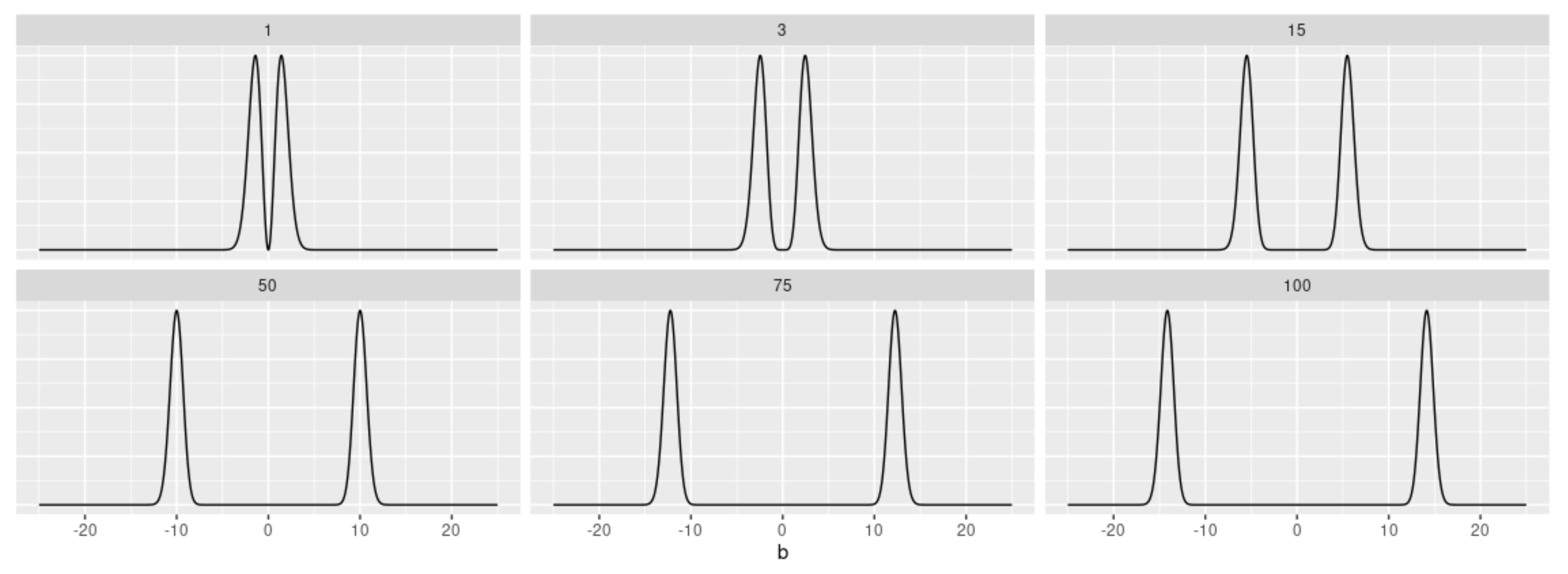
Definition 1. 
A random variable B is said to be distributed according to a Bimodal Normal (BN) distribution of order k, that is, B BN ( k ) (discussed in [22]), if its probability density function (PDF) is given by
f ( b k ) = 1 c b 2 k ϕ ( b ) , b R ,
in which ϕ ( · ) is the PDF of the standard normal distribution, c = j = 1 k ( 2 j 1 ) and k = { 1 , 2 , 3 , } .
This class of distributions is always bimodal, which means that the observed modes move away from each other when the order k increases (as depicted by Figure 1).
It is noteworthy mentioning that transformations derived from the BN ( k ) distribution may lead to other domains of interest, e.g., the unit domain. For example, let B BN ( k ) , then a scale parameter α , the transformation α | B | R + , and then the transformation e α | B | [ 0 , 1 ] . Thus, the stochastic characterization of a BN ( k ) distribution can be obtained according to the following theorem.
Theorem 1. 
Let W 1 and W 2 be independent random variables, in which W 1 is such that P ( W 1 = 1 ) = P ( W 1 = 1 ) = 1 / 2 and W 2 χ 2 k + 1 2 . Then,
W 1 W 2 BN ( k ) .
So, this theorem is mainly motivated by the result that shows that if X BN ( k ) , then X 2 χ 2 k + 1 2 . The entire demonstration is presented in Appendix A.

2. The Model

In this section, a new unit distribution, named Alpha-Unit, which presents a single parameter, α , is discussed. Its stochastic representations (probability density and cumulative distribution functions), moments (including mean and variance), moment-generating function, and how to generate pseudo-random numbers from it will be presented. Moreover, a proposal of statistical control chart for unit data based on the Alpha-Unit distribution will also be shown.
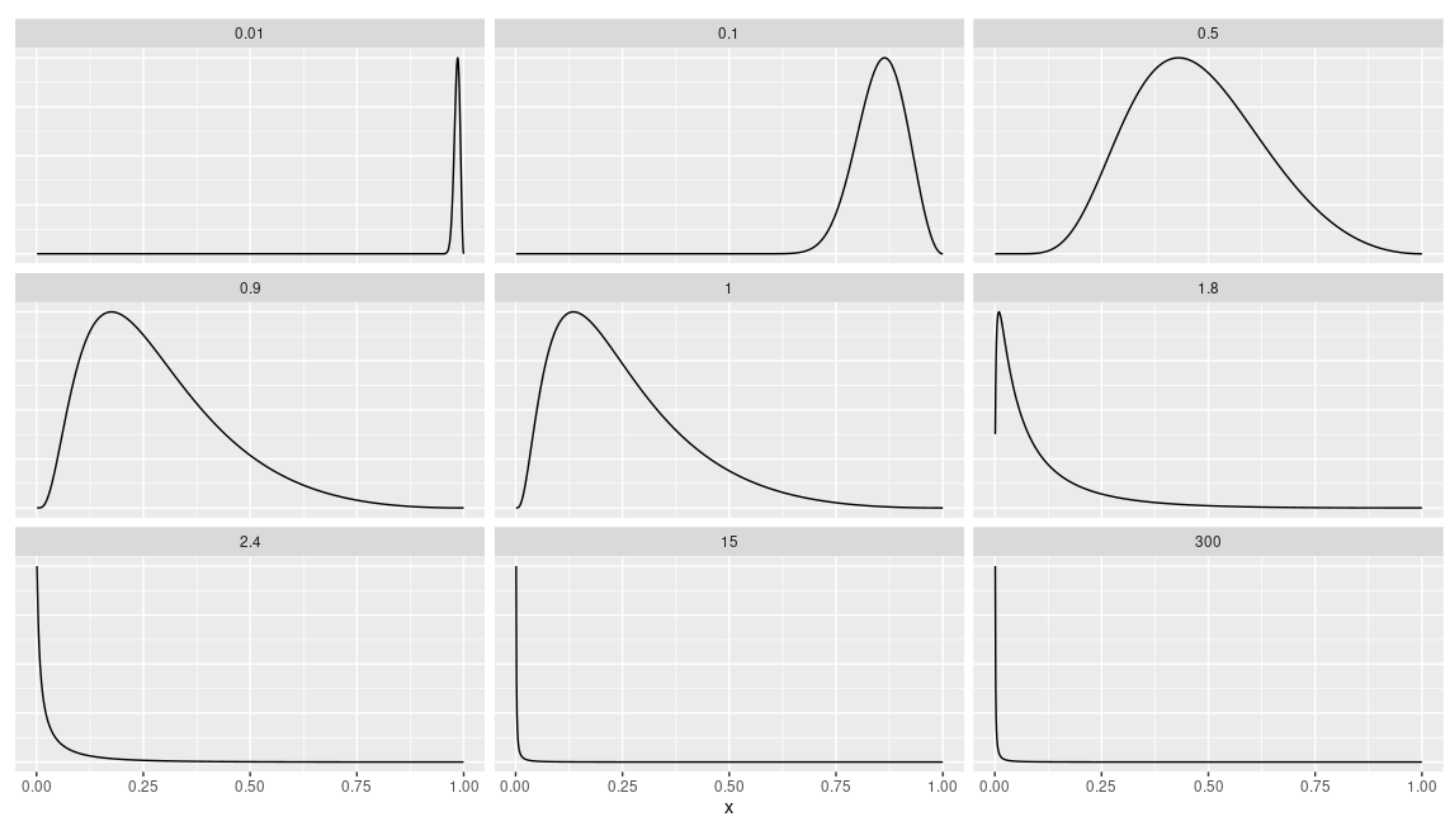
The Alpha-Unit density is originated from the general theorem (Theorem 1), by considering k = 1 . Moreover, it represents the second moment of the standard normal distribution and, later, transformed its domain. However, as k increases, the concentration of the distribution intensifies and other densities could be obtained.

Properties and Characterization

Definition 2. 
(Alpha-Unit distribution). A random variable X follows an Alpha-Unit (AU) distribution with parameter α > 0 , that is, X A U ( α ) , if its PDF is given by
f X ( x α ) = 2 x α ln ( x ) α 2 ϕ ln ( x ) α , 0 < x 1 .
Remark 1. 
If X A U ( α ) , then its PDF is unimodal.
Proof. 
The maxima of the AU distribution are studied, to which the criterion of the first derivative is first considered:
d f X ( x α ) d x = 2 x α 2 ln ( x ) α ϕ ln ( x ) α 2 x ln ( x ) x [ ln ( x ) ] 2 α 1 x α = 0 .
By solving algebraically for x, we obtain:
x = e α 2 + α 4 + 8 α 2 2 ( i ) e α 2 α 4 + 8 α 2 2 ( ii ) .
By working algebraically, it can be seen that this is only true for (ii), and is a global maximum, given that the solution is in between 0 and 1. Therefore, the AU distribution is unimodal.    □
Proposition 1. 
If X AU ( α ) , then itsr-th order moment is given by
E [ X r ] = 2 e r 2 α 2 2 1 + r 2 α 2 1 Φ ( r α ) r α ϕ ( r α ) ,
in which Φ ( · ) is the cumulative distribution function (CDF) of the standard normal distribution.
Proof. 
From the definition of the r-th order moment, we have:
E [ X r ] = 0 1 x r f X ( x α ) d x = 0 1 x r 2 x α ln ( x ) α 2 ϕ ln ( x ) α d x .
By changing the variables:
u = 1 α ln ( x ) e u α = x d u = 1 α x d x α e u α d u = d x ,
then substituting into Equation (3) and developing algebraically, we obtain:
E [ X r ] = 2 e α 2 r 2 2 0 u 2 1 2 π e ( u α r ) 2 2 d u .
Then, by making another change of variables: h = u α r , d h = d u ; and replacing these expressions in the previous equation, we have:
E [ X r ] = 2 e α 2 r 2 2 α r h + α r 2 1 2 π e h 2 2 d h = 2 e α 2 r 2 2 α r h 2 + 2 h α r + α 2 r 2 ϕ ( h ) d h = 2 e α 2 r 2 2 α r h 2 ϕ ( h ) d h + 2 α r α r h ϕ ( h ) d h + α 2 r 2 α r ϕ ( h ) d h .
By solving the integrals, we get to:
E [ X r ] = 2 e α 2 r 2 2 α r ϕ ( α r ) + 1 Φ ( α r ) 2 α r ϕ ( α r ) + α 2 r 2 1 Φ ( α r ) .
Then, by solving algebraically, we go down to the expression of Proposition 1.    □
Out of Proposition 1, we obtain the mean and variance of the AU ( α ) model as it follows:
E [ X ] = 2 e α 2 2 ( 1 + α 2 ) 1 Φ ( α ) α ϕ ( α ) , V ar [ X ] = E [ X 2 ] E [ X ] 2 = 2 e 2 α 2 ( 1 + 4 α 2 ) 1 Φ ( 2 α ) 2 α ϕ ( 2 α ) 4 e α 2 ( 1 + α 2 ) 1 Φ ( α ) α ϕ ( α ) 2 .
Remark 2. 
As an illustration, Figure 2 displays the generated asymmetry and kurtosis based on the chosen α parameter of the AU distribution.
Proposition 2. 
If X AU ( α ) , then its CDF is given by
F X ( x α ) = 2 Φ ln ( x ) α 2 ln ( x ) α ϕ ln ( x ) α .
Proof. 
By definition, the CDF is:
F X ( x α ) = 0 x 2 t α ln ( t ) α 2 ϕ ln ( t ) α d t .
By making the change of variables:
u = ln ( t ) α e u α = t d u = 1 α t d t α e u α d u = d t ,
then substituting into Equation (4) and reducing expressions algebraically, we get to:
F X ( x α ) = 2 ln ( x ) α u 2 ϕ ( u ) d u .
By calculating the integral, we find:
F X ( x α ) = 2 u ϕ ( u ) | ln ( x ) / α + ln ( x ) / α ϕ ( u ) d u = 2 ln ( x ) α ϕ ln ( x ) α + Φ ln ( x ) α .
Then, by multiplying and commuting, we get to the expression of Proposition 2.    □
Additionally, if X denotes the monitored variable, then the PDF of X is given by (2). Also, consider that the probability of false alarm (known as type I error) is π . Thus, we get to:
P ( X < LCL α ) = P ( X > UCL α ) = π / 2 ,
in which α is the in-control process parameter (that is, the parameter that controls the quality characteristic based on the in-control state), and LCL and UCL are the lower and upper control chart limits, respectively. Given the CDF F X ( x α ) , then the quantile function of X is defined by Q ( p α ) = F X 1 ( p α ) , 0 < p < 1 , which can be obtained by setting to zero and solving (numerically) for x the following equation:
Φ ln ( x ) α ln ( x ) α ϕ ln ( x ) α p 2 , for 0 < p < 1 .
Following [23], the control limits and centerline (CL) of the proposed control chart for unit data based on the AU distribution or, simply, AU control chart, are given by
LCL = Q π / 2 α , CL = E [ X α ] , UCL = Q 1 π / 2 α ,
in which Q ( . ) is the quantile function of the AU ( α ) distribution.
Proposition 3. 
If X AU ( α ) , then its moment-generating function (MGF) is given by
ψ X ( t α ) = 2 k = 0 t k k ! e k 2 α 2 2 1 + k 2 α 2 1 Φ ( k α ) k α ϕ ( k α ) .
Proof. 
By definition, the MGF is:
ψ X ( t α ) = E e t x = 0 1 e t x 2 x α ln ( x ) α 2 ϕ ln ( x ) α d x .
By making the following change of variables:
u = ln ( x ) α e u α = x d u = 1 α x d x α e u α d u = d x ,
then substituting and simplifying into Equation (5), we get to:
ψ X ( t α ) = 2 0 e t e u α u 2 ϕ ( u ) d u = 2 0 k = 0 t k e u α k k ! u 2 ϕ ( u ) d u .
Working algebraically, we obtain:
ψ X ( t α ) = 2 k = 0 t k k ! e α 2 k 2 2 0 u 2 1 2 π e ( u α k ) 2 2 d u .
By making the following change of variables: h = u α k , d h = d u ; then substituting it into the previous equation, we get to:
ψ X ( t α ) = 2 k = 0 t k k ! e α 2 k 2 2 α k ( h + α k ) 2 ϕ ( h ) d h .
Then, by solving the integral and adjusting algebraically, we get to the expression of Proposition 3.    □
The pseudo-code presented in Algorithm 1 describes the important steps for the generation of random (in fact, pseudo-random) numbers from the AU ( α ) distribution. Further proofs are attached under Appendix B.
Algorithm 1 Random number generation from the AU ( α ) model.
  • Step 1.Generate a random number x 1 χ 3 2 .
     
  • Step 2. Generate a random number u Uniform ( 0 , 1 ) . If u 1 / 2 , set v = X 1 ; otherwise, v = x 1 .
     
  • Step 3. Based on the numbers obtained, generate y = α | v | , in which α is a (positive) scale parameter and | v | follows a Bimodal Half-Normal (BHN) distribution.
     
  • Step 4. Conclude with the number generated by Step 3 as a negative power of base e, that is, x = e y = e α | v | [ 0 , 1 ] .
     
  • Step 5. Repeat Steps 1–4 n times to obtain a random sample of size n from the AU ( α ) model.

3. Inference

In this section, the parameter estimation adopting the UMVUE and MLE approaches are discussed. At first, it will be demonstrated that the UMVUE can be obtained straightforwardly, since the proposed AU distribution is part of the exponential family. Later, the MLE will also be discussed, which will help to estimate not only the point estimation of the α parameter, but also the interval estimation. We enrolled the reasoning considering the asymptotic convergence in distribution of the parameter estimator, as well as adapted a transformation that ensures that the interval of the parameter will always be on its domain (the delta method). The delta transformation procedure will enable the correct inferences and the standard error calculation associated with the parameter estimate. Later on, a simulation study to illustrate these theoretical results is presented.

3.1. UMVUE through the Exponential Family

Many of the distributions used in statistics belong to the exponential family, thereby implying in a considerable advantage over other models that do not belong to this family. Such an advantage is significantly declared when it comes to calculating the statistic T ( X ) of a random sample X = X 1 , X 2 , , X n . Next, it is shown that the proposed AU ( α ) distribution belongs to this family.
A random variable X is said to belong to the one-parameter exponential family if its associated PDF f ( · θ ) can be written in the form of:
f ( x θ ) = exp c ( θ ) T ( x ) + d ( θ ) + S ( x ) .
Let X AU ( α ) , then the PDF of X can be written in exponential form as it follows:
f ( x α ) = exp 1 2 α 2 [ ln ( x ) ] 2 3 ln ( α ) + ln [ ln ( x ) ] 2 x 2 π .
Then, X belongs to the one-parameter exponential family if we define:
c ( α ) = 1 2 α 2 , T ( x ) = [ ln ( x ) ] 2 , d ( α ) = 3 ln ( α ) , S ( x ) = ln [ ln ( x ) ] 2 x 2 π .
Let x = x 1 , x 2 , , x n be an observation (or realization) of the random sample X = X 1 , X 2 , , X n , with X i AU ( α ) , for i = 1 , 2 , , n . Then, the joint PDF presented in exponential form is
f ( x α ) = exp 1 2 α 2 i = 1 n [ ln ( x i ) ] 2 3 n ln ( α ) + i = 1 n ln [ ln ( x i ) ] 2 x i 2 π ,
from which it can be concluded that the statistic T ( X ) = i = 1 n [ ln ( X i ) ] 2 is sufficient and complete, once the AU distribution is part of the exponential family.
Proposition 4. 
Let X = X 1 , X 2 , , X n be a random sample, with X i AU ( α ) , for i = 1 , 2 , , n , and T ( X ) = i = 1 n [ ln ( X i ) ] 2 . Then,
W n = 1 α 2 T ( X ) χ 3 n 2 .
Proof. 
If G = ln ( X ) α 2 , then G χ 3 2 . Thus, n independent and identically distributed samples of G will have the sum of n χ 3 2 , which will result in a chi-squared distribution with degrees of freedom equal to 3 n , that is, χ 3 n 2 , since
F G ( g ) = P ( G g ) = P ln ( X ) α 2 g = P g ln ( X ) α g = P α g ln ( X ) α g = P ln ( X ) α g P ln ( X ) α g = 1 P ln ( X ) α g = 1 P X e α g = 1 F X e α g ,
so,
f G ( g ) = d F G ( g ) d g = f X e α g e α g α 2 g = 2 α e α g α g α 2 ϕ α g α e α g α 2 g = 1 g g 2 1 2 π e ( g ) 2 2 = 1 2 π g 1 / 2 exp g / 2 χ 3 2 .
Proposition 5. 
Let X = X 1 , X 2 , , X n be a random sample, with X i AU ( α ) , for i = 1 , 2 , , n , and T ( X ) = i = 1 n [ ln ( X i ) ] 2 . Then,
S ( X ) = Γ 3 n 2 2 Γ 3 n + 1 2 T ( X )
is an unbiased estimator of α .
Proof. 
First, remember that if X Gamma ( a , b ) distribution, then E [ X k ] = Γ ( a + b ) b k Γ ( a ) . Since the α parameter is observed to be squared, it will be necessary to apply it to find an unbiased estimator. So, considering the random variable W n 1 / 2 (with W n as defined in Proposition 4), it follows that:
E ( W n ) 1 / 2 = Γ 3 n 2 + 1 2 2 1 / 2 Γ 3 n 2 ,
so,
E 1 α 2 T ( X ) 1 / 2 = Γ 3 n 2 + 1 2 2 1 / 2 Γ 3 n 2 E T ( X ) Γ 3 n 2 2 Γ 3 n 2 + 1 2 S ( X ) = α .
Remark 3. 
Considering the two previous propositions and resorting to the Lehmann-Scheffé theorem, one can conclude that S ( X ) is UMVUE for α.

3.2. Estimation using the Maximum Likelihood Method

Let x = x 1 , x 2 , , x n be a realization of the random sample X = X 1 , X 2 , , X n taken from the AU ( α ) distribution. Then, the log-likelihood function is given by
( α ) = constant 3 n ln ( α ) Σ i = 1 n ln ( x i ) + 2 Σ i = 1 n ln ( ln ( x i ) ) 1 2 α 2 Σ i = 1 n [ ln ( x i ) ] 2 .
The MLE of α , i.e., α ^ , is found by solving the following equation:
d ( α ) d α = 3 n α + 1 α 3 Σ i = 1 n [ ln ( x i ) ] 2 = 0 ,
resulting
α ^ = 1 3 n i = 1 n [ ln ( x i ) ] 2 1 / 2 .
On the other hand, the second derivative of ( α ) evaluated at α = α ^ is negative, therefore concluding that α ^ is MLE for α .
It is known that, under certain regularity conditions,
n α ^ α D N 0 , I 1 ( α ) ,
in which I ( α ) = E d 2 ( α ) d α 2 = 6 n α 2 .
A two-sided 100 ( 1 π ) % confidence interval for α can be calculated by
α ^ z 1 π / 2 V ar α ^ , α ^ + z 1 π / 2 V ar α ^ ,
in which z q is the q-th percentile of the standard normal distribution. The variance of α ^ can be approximated by the inverse of the observed Fisher information, as
V ar α ^ = I 1 α ^ = α ^ 2 6 n .
Since α is a positive value and we cannot guarantee that the lower limit of the interval (6) is positive, we resort to the delta method to remedy such situation. For this, we define the function g : [ 0 , ) R as g ( α ) = ln ( α ) , and knowing that
n g ( α ^ ) g ( α ) D N 0 , I 1 α d g α d α 2 ,
we can, then, obtain an approximate two-sided 100 ( 1 π ) % confidence interval for α through
α ^ exp z 1 π / 2 6 n , α ^ exp z 1 π / 2 6 n .

3.3. Simulation Study

In order to illustrate the presented inferences for the estimation of the AU distribution, the MLE versus the UMVUE are compared (via simulation study) in this subsection. Moreover, we considered the scenarios in which the parameter α = { 0.1 , 0.3 , 0.5 , 0.7 , 1.1 , 1.5 } , considering sample sizes n = { 100 , 200 , 500 } , through the Monte Carlo method with N = 1000 repetitions. This entire procedure took into account the random number generator for the AU ( α ) distribution shown in Algorithm 1. All analyses carried out in this study adopted the open-source R software [24].
For the performance comparison of the proposed estimators (MLE and UMVUE), since the true parameter value is known, the bias and mean squared error (MSE) metrics were adopted, and they are defined, respectively, as it follows:
Bias ( α ) = 1 N i = 1 N ( α ^ i α ) and MSE ( α ) = 1 N i = 1 N ( α ^ i α ) 2 ,
in which α ^ i is the estimate for α in the i-th iteration (point estimation). Additionally, based on the asymptotic results presented in this study, we also calculated the 95% confidence interval (CI) length by adopting the delta method from Equation (7) (interval estimation). That is, it analyzed the average of all the upper limits of the 95% confidence interval, as well as the average of all the lower limits, and then calculated their difference.
Table 1 presents the obtained average estimates (AvE) of the α parameter, for each sample size n, as well as the corresponding bias, MSE and 95% CI length (this last one only for MLE) results.
The asymptotic convergence of the MLE towards the robustness is noticed as the sample size increases. In addition, both MLE and UMVUE’s bias and MSE are small and tend to decrease as n gets larger. On the other hand, the CI length also decreases as the sample size increases.
Finally, regarding the robustness of the estimators, the difference between the MLE and UMVUE estimates was taken, considering each different sample size n. Then, the interquartile range (IQR) was calculated per sample size group. That is, IQR ( n i ) α 1 ^ MLE ( n i ) α 1 ^ UMVUE ( n i ) , , α j ^ MLE ( n i ) α j ^ UMVUE ( n i ) , , α 6 ^ MLE ( n i ) α 6 ^ UMVUE ( n i ) , in which n i = { 100 , 200 , 500 } and α j = { α 1 = 0.1 , α 2 = 0.3 , , α 6 = 1.5 } . For instance, the IQR for n = 100 was 0.00053 , whereas for n = 200 and n = 500 , it went down to 0.00025 and 0.00012 , respectively. This points out, in short, that as the sample size gets larger, the error range gets smaller, regardless of the value of the α parameter.

4. Real-World Exemplifications

In this section, two applications adopting the AU distribution with real-world issues are exemplified. The first case is related to the dynamics of the Chilean inflation in the post-military dictatorship period. The second case pertains to the relative humidity of the air in the northern Chilean city of Copiapó (Atacama region).
The Chilean inflation data are recorded annually, whose values considered the range from 1992 to 2021. These are based on the period after the military dictatorship of 1973–1990. It was analyzed the dynamics of the inflation data (in %), which were standardized by min-max transformation, resulting in a unit response variable (value between zero and one). The years 1990 and 1991 were excluded, since they are considered to be a period of transition. Then, the total amount of observations was of 30 years (from 1992 to 2021).
On the other hand, the relative air humidity data cover the period from February 2015 to October 2022, with a one-hour recording format (104,415 observations). Then, this data set was transformed into daily maximum observation (6226 observations).

4.1. Chilean Inflation (Post-Military Era)

Figure 3 presents the dynamics of the Chilean inflation in the post-military dictatorship period, demonstrating stability between the years of 1999 and 2008. The right panel displays the time series of inflation, in which time is measured in years, from year 1 (1992) to year 30 (2021). The left panel depicts the accumulation of the values throughout the time series, in which a predominant trend is shown around 0.1 of the inflation rate.
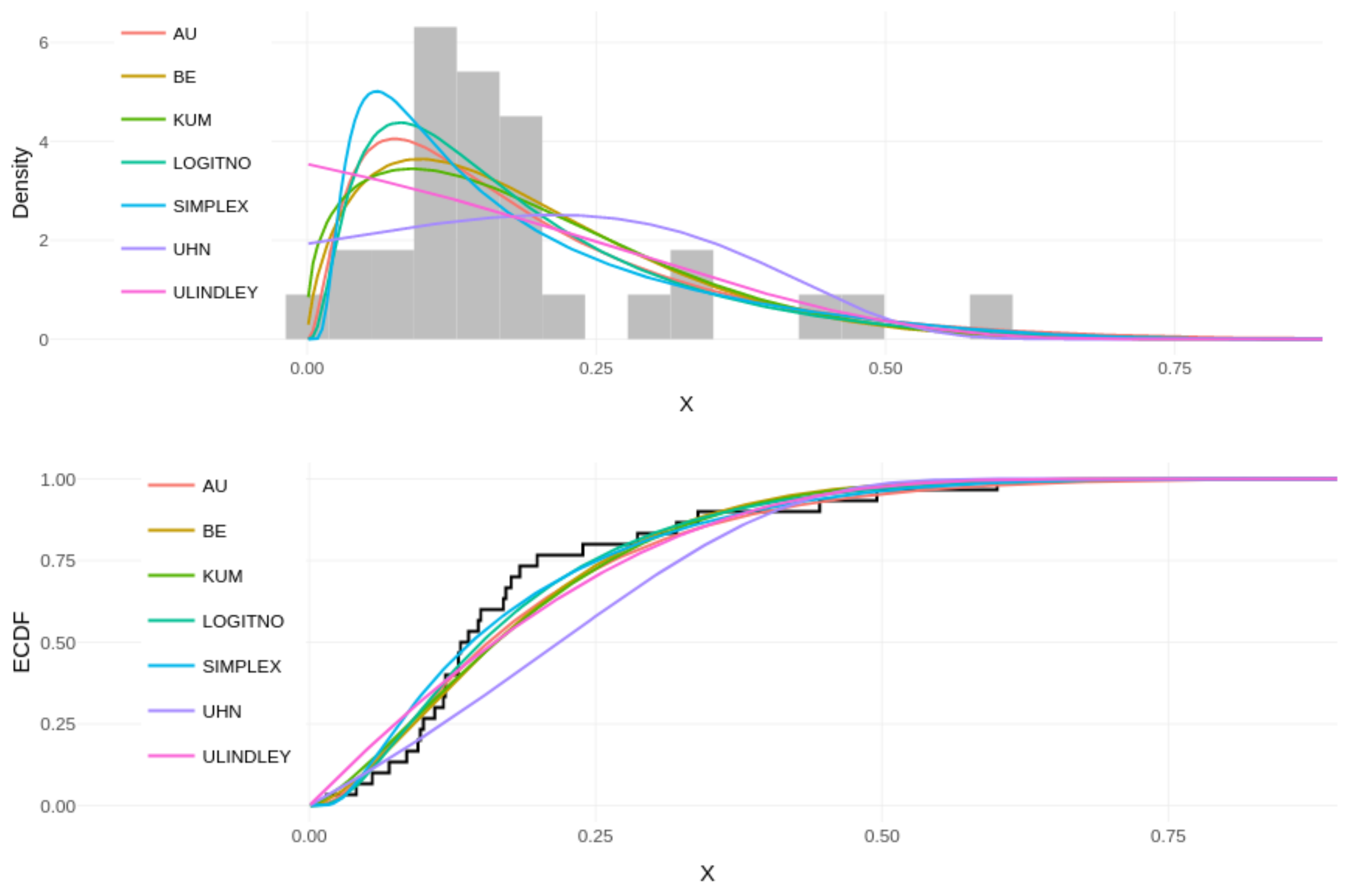
Once the empirical dynamics of these data was analyzed, the most common unit distributions, presented in the statistical literature, were fitted. The upper panel of Figure 4 illustrates the histogram for the inflation data, in which it is compared with different fitted densities based on the MLE: AU, beta (BE), Kumaraswamy (KUM), logit-normal (LOGITNO), simplex (SIMPLEX), unit-half-normal (UHN), and unit-Lindley (ULINDLEY). The lower panel of the same figure presents the fitted CDFs superimposed to the empirical CDF (ECDF).
In order to quantify the performance of the fitted models, the Akaike Information Criterion (AIC) [25] and the Bayesian (or Schwarz) Information Criterion (BIC) [26] were analyzed. The obtained results (see Table 2) indicated the AU model as the best-fitted model to this data set. In addition, it is possible to make an inference about the average of the phenomenon, that is, the expectation of the AU( α ^ = 1.2059 ) model, resulting in E [ X Inflation ] = 0.1948 . In other words, the average Chilean inflation, in post-military era, is of 19.49%.
In the following subsection, it is illustrated the performance of the AU model when adopting a high-frequency data set originated from the relative humidity from a city located in the Atacama Desert.

4.2. Water Monitoring in Air Humidity

The hydrological regime of the main rivers of Atacama is characterized by ice sources: water flows from the peaks following the melting of snowfall, glaciers, and permafrost located in the upper parts of the Andes range. In the context of climate change, it is, therefore, essential to understand the hydrological cycle of these regions, in order to set up a sustainable management policy to them. Understanding the hydrological cycle requires the implementation of tools for forecasting river flows, relative humidity, groundwater reservoirs, or any other water-related quantity monitoring, which inevitably demands an in-depth knowledge with respect to the physical phenomena that rule the entire hydrological cycle and, more precisely, the complex interaction between atmosphere, climate, landforms, ice, snow and river flows.
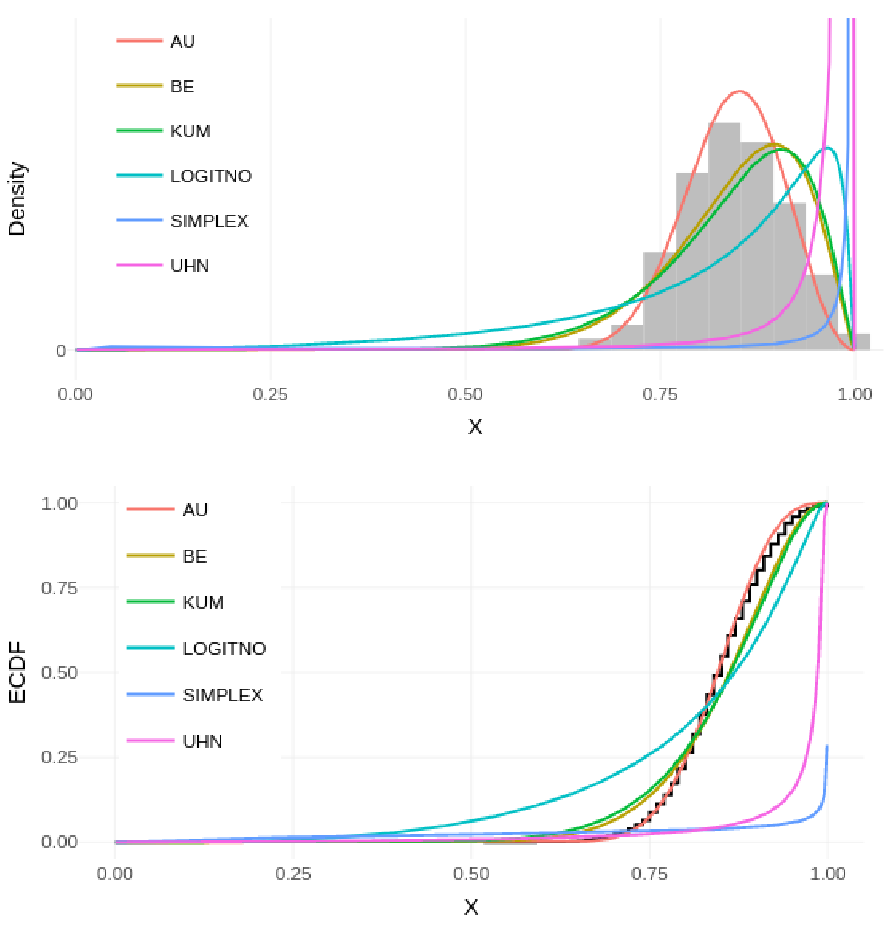
Additionally, a unique phenomenon called Camanchaca happens, which consists in a fog passing by the Copiapó city, recurrent only between midnight to around 10 a.m. Here, we demonstrate the variation of the relative humidity of Copiapó city, proposing a methodology that can be efficient, adjustable to these data. Using the daily maximum relative humidity, six different unit distributions were compared: AU, BE, KUM, LOGITNO, SIMPLEX, and UHN, as shown in Figure 5.
After comparing the commonly used unit models, we demonstrate the advantage of fitting the AU model over others (visually). Table 3 confirms the best fit of the AU model, based on information criteria (AIC and BIC), as well as depicts the estimation of the parameter(s) of each model.
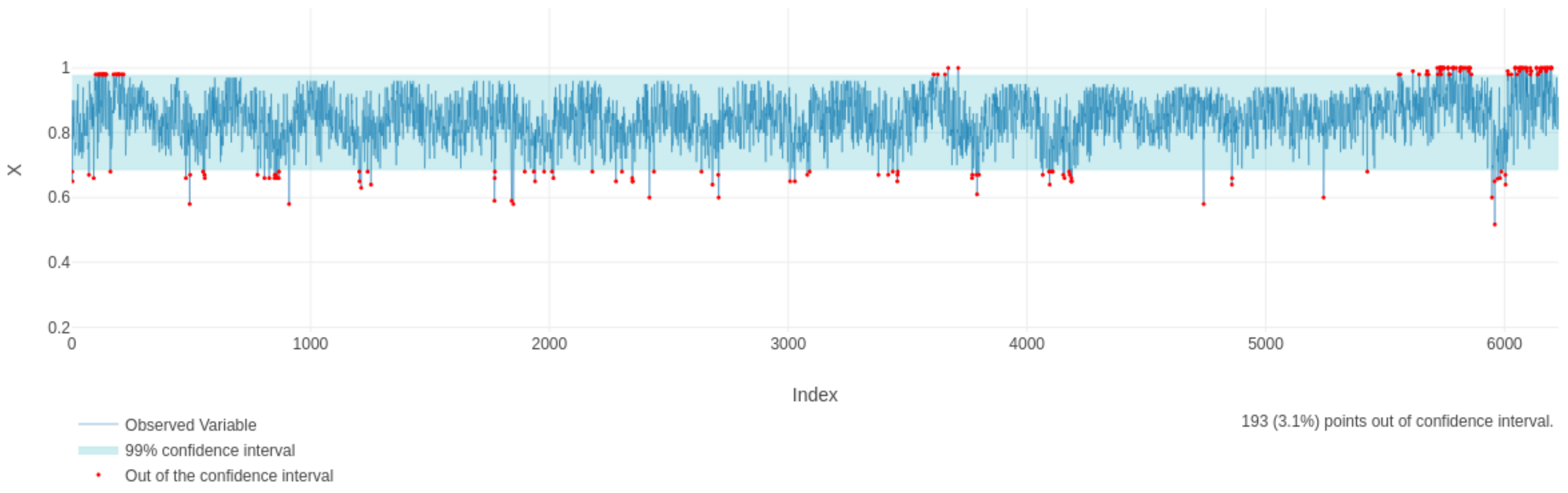
After obtaining the parameter estimate for α , the AU model (best-fitted model) was used to construct a Statistical Process Control (SPC) chart [27], by calculating a tolerance upper-lower bound. Moreover, the Highest Density Interval (HDI) was adopted, considering a confidence degree of 99%, to monitor the daily maximum relative humidity records (as displayed by Figure 6).
The expected daily maximum water relative humidity is of 84.23% (based on the fitted AU model). The obtained control limits, considering a confidence (or tolerance) level of 99%, were: LCL = 68.56 % and UCL = 97.73 % . Thus, the control chart based on the AU model (AU control chart) is another exciting and valuable alternative to some well-known SPC tools, which enlightens the forecasting and opens new doors to discuss extreme events in the Atacama water particles monitored by probabilistic reasoning.

5. Conclusions

This study showed the competitiveness of the developed Theorem 1 (Equation (1)), which enables for a great class of distributions that belong all to the exponential family. As an exemplification, we adopted the special case for k = 1 , which is equivalent to the moment of order two of the standard normal distribution, and after some transformations, we developed the Alpha-Unit (AU) distribution. Also, we dedicated to the unit range, given the importance of this stochasticity representation.
Unit distributions are useful for values that oscillate between zero and one, such as fractions, proportions and rates, among others, or for a set of values in which there is a minimum or maximum limitation, resorting to standardization through the min-max transformation. Most distributions of this type come from transforming a random variable with certain distribution so that it takes values between zero and one, as in the case of unit-Lindley distribution [9], which comes from the Lindley distribution [28,29].
There are numerous studies based on (e.g., unit) distributions, by extending a model and applying it to several areas [11,14,16]. In this study, we introduced and showed the competitiveness of the AU distribution, especially for data with a range greater than 0.4, or which present high asymmetry and low decay. Further studies shall investigate this hypothesis in a wider amount of data sets (through different sorts of wide data range). Additionally, an implementation of this model adopting hierarchical estimation and spatio-temporal dependence would be useful for forecast/predictable problems.

Author Contributions

Conceptualization and methodology, D.E.-O. and D.C.d.N.; software, M.S.C.-A. and L.B.-B.; validation, formal analysis, investigation, resources, data curation, M.S.C.-A. and D.C.d.N.; writing—original draft preparation, D.E.-O., D.C.d.N., M.S.C.-A. and L.B.-B.; writing—review and editing, P.H.F.d.S.; visualization, D.C.d.N.; supervision, project administration, funding acquisition, D.E.-O. All authors have read and agreed to the published version of the manuscript.

Funding

This research was funded by Universidad de Atacama grant number ATA1956–CC88433.

Institutional Review Board Statement

Not applicable.

Informed Consent Statement

Not applicable.

Data Availability Statement

All adopted data and R script developed in this study are available at https://github.com/ProfNascimento/AlphaUnit (accessed on 12 November 2022).

Acknowledgments

This study was partially supported by the Vicerrectoría de Investigación y Postgrado (VRIP) and Dirección de Postgrado of the Universidad de Atacama (UDA). The author David Elal-Olivero was supported by the DIUDA REGULAR project No. 22409 from the Universidad de Atacama, Chile.

Conflicts of Interest

The authors declare no conflict of interest.

Appendix A

This appendix shows the proof that for a random variable
X BN ( k ) X 2 χ 2 k + 1 2 .
Then,
F X 2 ( x ) = P X 2 x = P x X x = 2 P X x 1 = 2 F X x 1 .
It follows that
f X 2 ( x ) = 2 f X x 1 2 x = 1 c x 2 k ϕ ( x ) 1 x = 1 j = 1 k ( 2 j 1 ) x 2 k 1 1 2 π e x 2 .
Knowing that Γ 2 k + 1 2 = j = 1 k ( 2 j 1 ) π 2 k , then
f X 2 ( x ) = 1 j = 1 k ( 2 j 1 ) x 2 k 1 2 1 2 π e x 2 = π 2 k Γ 2 k + 1 2 x 2 k 1 2 2 1 / 2 π e x 2 = 1 Γ 2 k + 1 2 2 2 k + 1 2 x 2 k 1 2 e x 2 .
Therefore, X 2 χ 2 k + 1 2 .
Besides that, complementation can be taken into account by saying that, considering W 2 χ 2 k + 1 2 and P ( W 1 = ± 1 ) = 1 / 2 , then B = W 1 W 2 BN ( k ) .
Let b 0 , then
F B ( b ) = P ( B b ) = P W 1 W 2 b = P W 1 W 2 b W 1 = 1 P W 1 = 1 + P W 1 W 2 b W 1 = 1 P W 1 = 1 = ind . P ( 1 ) W 2 b 1 2 + P ( 1 ) W 2 b 1 2 . Sin ce b 0 , then P ( 1 ) W 2 b = 1 : = P W 2 b 1 2 + 1 2 = P | W 2 | b 2 1 2 + 1 2 = P b 2 W 2 b 2 1 2 + 1 2 = 1 2 P X b 2 P X b 2 0 + 1 2 = 1 2 P X b 2 + 1 2 = 1 2 F X b 2 + 1 2
Therefore,
f B ( b ) = d F B ( b ) d b = 1 2 f X b 2 2 b = b f X b 2 = b 1 Γ 2 k + 1 2 2 2 k + 1 2 b 2 2 k + 1 2 1 e b 2 2 = b 1 Γ 2 k + 1 2 2 2 k + 1 2 b 2 k 1 e b 2 2 = 1 π j = 1 k ( 2 j 1 ) 2 k 2 2 k + 1 2 b 2 k e b 2 2 = 1 j = 1 k ( 2 j 1 ) b 2 k 2 π e b 2 2 = 1 j = 1 k ( 2 j 1 ) c b 2 k ϕ ( b ) .
Analogously, it is proved for b < 0 .

Appendix B

The proposed theorem (Theorem 1) will be illustrated considering k = 1 , to show the origin of the random numbers that generate the AU distribution.
Proposition A1. 
If X BN ( 1 ) , then f X ( x ) = x 2 ϕ ( x ) is a bimodal density function.
Proof. 
If f X ( x ) is bimodal, it would have two maxima, to which the first and second derivative criteria would be applied:
d f X ( x ) d x = 0
d x 2 ϕ ( x ) d x = 2 x ϕ ( x ) + x 2 x ϕ ( x ) = 2 x ϕ ( x ) x 3 ϕ ( x ) = x ϕ ( x ) 2 x 2 = 0 .
Then, it can be seen that the solutions for the previous equation would be: x 1 = 0 , x 2 = 2 , x 3 = 2 . Hence, by applying the second derivative criterion:
d 2 f X ( x ) d x 2 < 0
d x ϕ ( x ) 2 x 2 d x = ϕ ( x ) 2 x 2 + x x ϕ ( x ) 2 x 2 + x ϕ ( x ) ( 2 x ) .
Reducing algebraically, we get to:
d 2 f X ( x ) d x 2 = ϕ ( x ) 2 5 x 2 + x 4 < 0 .
The only solutions that satisfy the previous inequality are: x 2 = 2 , x 3 = 2 . Therefore, there are two maxima and the BN distribution is bimodal.
Definition A1 (Bimodal Half-Normal distribution).
Let Y BN ( 1 ) . If Q = α | Y | , with α > 0 , then we say that Q is distributed according to a Bimodal Half-Normal (BHN) distribution with parameter α, and we denote it by Q BHN ( α ) .
Proposition A2. 
If Q BHN ( α ) , then the PDF of Q is given by
f Q ( q α ) = 2 α q α 2 ϕ q α , q > 0 .
Proof. 
Since Q = α | Y | , with Y BN ( 1 ) , then
F Q ( q ) = P ( Q q ) = P ( α | Y | q ) = P q α Y q α = 2 P Y q α 1 = 2 F Y q α 1 .
Hence, by deriving the previous expression, one has that
f Q ( q ) = 2 f Y q α 1 α = 2 α q α 2 ϕ q α .
Proposition A3. 
If Q BHN ( α ) , then
X = e Q AU ( α ) .
Proof. 
Let X = e Q , 0 < x 1 , then
F X ( x ) = P ( X x ) = P e Q x = P Q ln ( x ) = P Q ln ( x ) = 1 P Q ln ( x ) = 1 F Q ln ( x ) .
By deriving the previous expression, we have:
f X ( x ) = f Q ( ln ( x ) ) 1 x = 2 α ln ( x ) α 2 ϕ ln ( x ) α 1 x = 2 α x ln ( x ) α 2 ϕ ln ( x ) α .

References

  1. Fonseca, A.; Ferreira, P.H.; Nascimento, D.C.d.; Fiaccone, R.; Ulloa-Correa, C.; García-Piña, A.; Louzada, F. Water particles monitoring in the atacama desert: SPC approach based on proportional data. Axioms 2021, 10, 154. [Google Scholar] [CrossRef]
  2. Bayer, F.M.; Cintra, R.J.; Cribari-Neto, F. Beta seasonal autoregressive moving average models. J. Stat. Comput. Simul. 2018, 88, 2961–2981. [Google Scholar] [CrossRef] [Green Version]
  3. Ferrari, S.; Cribari-Neto, F. Beta regression for modelling rates and proportions. J. Appl. Stat. 2004, 31, 799–815. [Google Scholar] [CrossRef]
  4. Kumaraswamy, P. A generalized probability density function for double-bounded random processes. J. Hydrol. 1980, 46, 79–88. [Google Scholar] [CrossRef]
  5. Tadikamalla, P.R.; Johnson, N.L. Systems of frequency curves generated by transformations of logistic variables. Biometrika 1982, 69, 461–465. [Google Scholar] [CrossRef]
  6. Barndorff-Nielsen, O.E.; Jørgensen, B. Some parametric models on the simplex. J. Multivar. Anal. 1991, 39, 106–116. [Google Scholar] [CrossRef] [Green Version]
  7. Mazucheli, J.; Menezes, A.F.B.; Ghitany, M.E. The unit-Weibull distribution and associated inference. J. Appl. Probab. Stat. 2018, 13, 1–22. [Google Scholar]
  8. Mazucheli, J.; Menezes, A.; Fernandes, L.; De Oliveira, R.; Ghitany, M. The unit-Weibull distribution as an alternative to the Kumaraswamy distribution for the modeling of quantiles conditional on covariates. J. Appl. Stat. 2020, 47, 954–974. [Google Scholar] [CrossRef]
  9. Mazucheli, J.; Menezes, A.F.B.; Chakraborty, S. On the one parameter unit-Lindley distribution and its associated regression model for proportion data. J. Appl. Stat. 2019, 46, 700–714. [Google Scholar] [CrossRef] [Green Version]
  10. Bakouch, H.S.; Nik, A.S.; Asgharzadeh, A.; Salinas, H.S. A flexible probability model for proportion data: Unit-half-normal distribution. Commun. Stat.-Case Stud. Data Anal. Appl. 2021, 7, 271–288. [Google Scholar] [CrossRef]
  11. Korkmaz, M.Ç.; Korkmaz, Z.S. The unit log–log distribution: A new unit distribution with alternative quantile regression modeling and educational measurements applications. J. Appl. Stat. 2021, 1, 1–20. [Google Scholar] [CrossRef]
  12. Sagrillo, M.; Guerra, R.R.; Bayer, F.M. Modified Kumaraswamy distributions for double bounded hydro-environmental data. J. Hydrol. 2021, 603, 127021. [Google Scholar] [CrossRef]
  13. Krishna, A.; Maya, R.; Chesneau, C.; Irshad, M.R. The Unit Teissier Distribution and Its Applications. Math. Comput. Appl. 2022, 27, 12. [Google Scholar] [CrossRef]
  14. Guerra, R.R.; Peña-Ramírez, F.A.; Bourguignon, M. The unit extended Weibull families of distributions and its applications. J. Appl. Stat. 2021, 48, 3174–3192. [Google Scholar] [CrossRef]
  15. Aitchison, J.; Brown, J.A.C. The Lognormal Distribution with Special Reference to Its Uses in Economics; Cambridge University Press: Cambridge, UK, 1957. [Google Scholar]
  16. Korkmaz, M.Ç.; Chesneau, C.; Korkmaz, Z.S. The Unit Folded Normal Distribution: A New Unit Probability Distribution with the Estimation Procedures, Quantile Regression Modeling and Educational Attainment Applications. J. Reliab. Stat. Stud. 2022, 15, 261–298. [Google Scholar] [CrossRef]
  17. Afify, A.Z.; Nassar, M.; Kumar, D.; Cordeiro, G.M. A new unit distribution: Properties, inference, and applications. Electron. J. Appl. Stat. Anal. 2022, 15, 460–484. [Google Scholar]
  18. Korkmaz, M.Ç.; Altun, E.; Chesneau, C.; Yousof, H.M. On the unit-Chen distribution with associated quantile regression and applications. Math. Slovaca 2022, 72, 765–786. [Google Scholar] [CrossRef]
  19. Santana-e Silva, J.J.; Cribari-Neto, F.; Vasconcellos, K.L. Beta distribution misspecification tests with application to Covid-19 mortality rates in the United States. PLoS ONE 2022, 17, e0274781. [Google Scholar] [CrossRef]
  20. Stahl, S. The evolution of the normal distribution. Math. Mag. 2006, 79, 96–113. [Google Scholar] [CrossRef]
  21. Limpert, E.; Stahel, W.A. Problems with using the normal distribution–and ways to improve quality and efficiency of data analysis. PLoS ONE 2011, 6, e21403. [Google Scholar] [CrossRef] [Green Version]
  22. Elal-Olivero, D. Alpha-skew-normal distribution. Proyecciones (Antofagasta) 2010, 29, 224–240. [Google Scholar] [CrossRef] [Green Version]
  23. Bayer, F.M.; Tondolo, C.M.; Müller, F.M. Beta regression control chart for monitoring fractions and proportions. Comput. Ind. Eng. 2018, 119, 416–426. [Google Scholar] [CrossRef]
  24. R Core Team. R: A Language and Environment for Statistical Computing; R Foundation for Statistical Computing: Vienna, Austria, 2022. [Google Scholar]
  25. Akaike, H. On entropy maximization principle. Appl. Stat. 1977, 1, 27–41. [Google Scholar]
  26. Schwarz, G. Estimating the dimension of a model. Ann. Stat. 1978, 6, 461–464. [Google Scholar] [CrossRef]
  27. Montgomery, D.C. Introduction to Statistical Quality Control, 6th ed.; John Wiley & Sons: Hoboken, NJ, USA, 2009. [Google Scholar]
  28. Lindley, D.V. Fiducial distributions and Bayes’ theorem. J. R. Stat. Soc. Ser. B (Methodol.) 1958, 20, 102–107. [Google Scholar] [CrossRef]
  29. Lindley, D.V. Introduction to Probability and Statistics from a Bayesian Viewpoint, Part II: Inference; Cambridge University Press: Cambridge, UK, 1965. [Google Scholar]
Figure 1. Density function of the BN distribution by varying the parameter k (displayed at the top of each chart).
Axioms 11 00666 g001
Figure 2. Density function of the AU distribution by varying the parameter α (displayed at the top of each chart). Whereas B BN ( 1 ) B 2 χ 3 2 , then the AU model was generated from X = e α | B | .
Axioms 11 00666 g002
Figure 3. Chilean inflation in the period 1992–2021 (post-military era). The histogram on the left presents a skewness of the data. The dynamics is represented in the right panel, in which a disturbance (outlier) is observed in the year 2008 (observation #17).
Axioms 11 00666 g003
Figure 4. Estimated densities superimposed to the histogram (top-chart), and estimated CDFs superimposed to the ECDF (bottom-chart) (Chilean inflation data).
Axioms 11 00666 g004
Figure 5. Estimated densities superimposed to the histogram (top-chart), and estimated CDFs superimposed to the ECDF (bottom-chart) (relative air humidity data).
Axioms 11 00666 g005
Figure 6. SPC control chart, considering a 99% of tolerance based on the AU model fitted to the daily maximum relative humidity of Copiapó city, Chile, from 1 February 2015 to 4 October 2022. It is observed that 193 days (3.1%) presented anomaly values (out-of-control signals). The obtained control limits were: LCL = 68.56 % and UCL = 97.73 % .
Axioms 11 00666 g006
Table 1. AvE, bias, MSE and 95% CI length (only for MLE) for the proposed estimators (MLE and UMVUE) of the single parameter ( α ) of the AU distribution, considering different sample sizes (n).
n α MLE UMVUE
AvEBiasMSECI LengthAvEBiasMSE
1000.10.0998−0.00021.6930 × 10 5 0.01600.0999−8.2264 × 10 5 1.6165 × 10 5
200 0.0999−9.8758 × 10 5 8.7306 × 10 6 0.01130.0999−5.7124 × 10 5 8.7314 × 10 6
500 0.0999−3.3400 × 10 6 3.5542 × 10 6 0.00710.10001.3327 × 10 5 3.5555 × 10 6
1000.30.2996−0.00040.00020.04800.2999−8.0656 × 10 5 0.0002
200 0.2997−0.00037.8575 × 10 5 0.03390.2998−0.00027.8582 × 10 5
500 0.2999−1.0020 × 10 5 3.1987 × 10 5 0.02140.30020.00023.0979 × 10 5
1000.50.4994−0.00060.00040.08000.4999−0.00010.0004
200 0.4997−0.00030.00020.05650.4997−0.00030.0002
500 0.4999−1.6700 × 10 5 8.8855 × 10 5 0.03570.50006.6637 × 10 5 8.8888 × 10 5
1000.70.6992−0.00080.00080.11200.6998−0.00020.0008
200 0.6993−0.00070.00040.07910.6996−0.00040.0004
500 0.6999−2.3380 × 10 5 0.00010.05010.70009.3291 × 10 5 0.0001
1001.11.0987−0.00130.00200.17601.0997−0.00030.0020
200 1.0989−0.00110.00100.12441.0994−0.00060.0010
500 1.0999−3.6741 × 10 5 0.00040.07871.10010.00010.0004
1001.51.4983−0.00170.00380.24001.4996−0.00040.0038
200 1.4985−0.00150.00190.16961.4991−0.00090.0019
500 1.4999−5.0101 × 10 5 0.00080.10731.50020.00020.0007
Table 2. Parameter estimates, AIC and BIC values (Chilean inflation data). S.E. = standard error.
ModelParameter Estimate (S.E.)AICBIC
AU ( α ) α ^ = 1.205943 ( 0.008079 ) 47.89 46.49
BE ( μ , σ ) μ ^ = 0.185857 ( 0.000496 ) 44.58 41.78
σ ^ = 0.314688 ( 0.001304 )
KUM ( μ , σ ) μ ^ = 1.370127 ( 0.045522 ) 43.63 40.83
σ ^ = 7.968427 ( 7.750459 )
LOGITNO ( μ , σ ) μ ^ = 0.150323 ( 0.000457 ) 46.23 43.43
σ ^ = 0.916938 ( 0.014013 )
SIMPLEX ( μ , σ ) μ ^ = 0.182462 ( 0.000584 ) 43.17 40.37
σ ^ = 2.854833 ( 0.135834 )
UHN ( σ ) σ ^ = 0.413894 ( 0.002855 ) 33.62 32.22
ULINDLEY ( μ ) μ ^ = 0.186834 ( 0.000575 ) 41.99 40.58
Table 3. Parameter estimates, AIC and BIC values (relative air humidity data).
ModelParameter Estimate (S.E.)AICBIC
AU ( α ) α ^ = 0.1092 ( 3.1902 × 10 7 ) 14 , 023.49 14 , 016.76
BE ( μ , σ ) μ ^ = 0.8476 ( 1.2027 × 10 6 ) 13 , 927.89 13 , 914.41
σ ^ = 0.2410 ( 4.1119 × 10 6 )
KUM ( μ , σ ) μ ^ = 9.4004 ( 0.0141 ) 13 , 605.90 13 , 592.43
σ ^ = 2.3882 ( 0.0019 )
LOGITNO ( μ , σ ) μ ^ = 0.8693 ( 3.1376 × 10 6 ) 7600.43 7586.95
σ ^ = 1.2299 ( 1.2148 × 10 4 )
SIMPLEX ( μ , σ ) μ ^ = 0.9735 ( 1.2959 × 10 6 ) 32 , 477.13 32,490.61
σ ^ = 94.0480 ( 0.7103 )
UHN ( σ ) σ ^ = 99.9900 ( 6.5334 × 10 7 ) 5,101,018,733.135,101,018,739.86
Publisher’s Note: MDPI stays neutral with regard to jurisdictional claims in published maps and institutional affiliations.

