

Solving Biharmonic Equations with Tri-Cubic C1 Splines on Unstructured Hex Meshes

Abstract
:1. Introduction
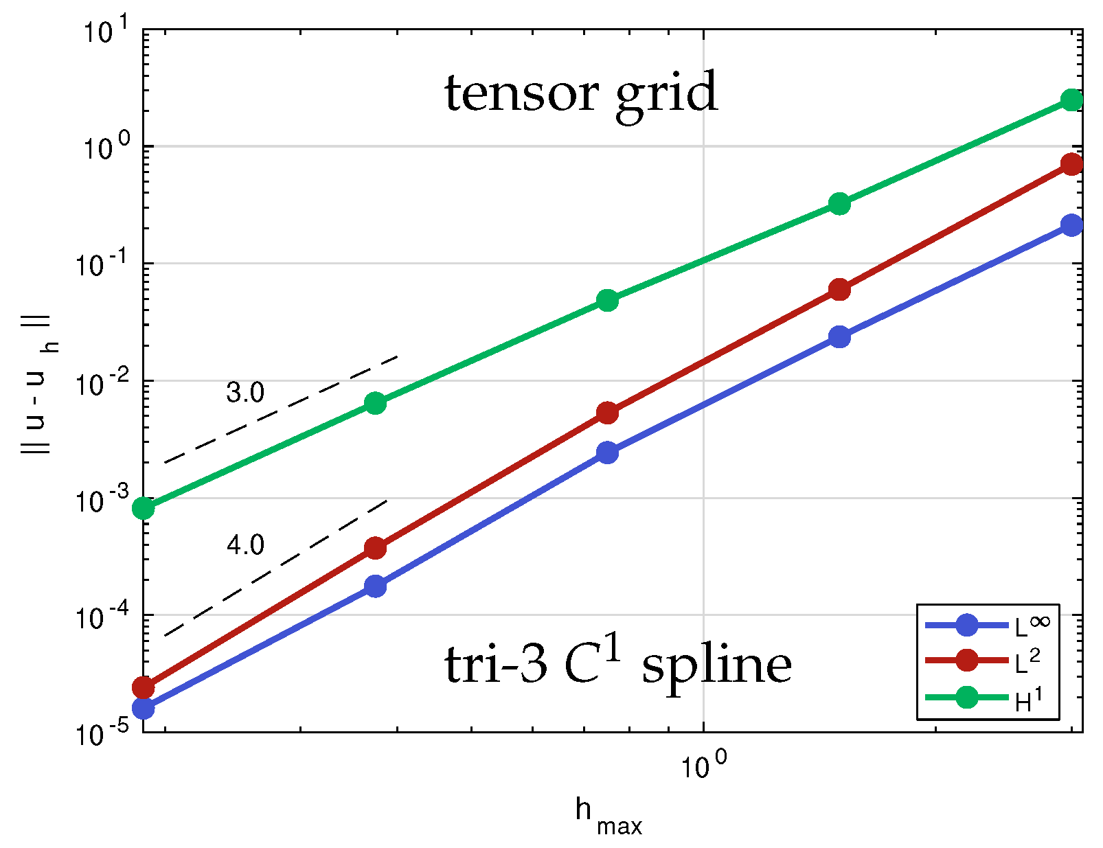
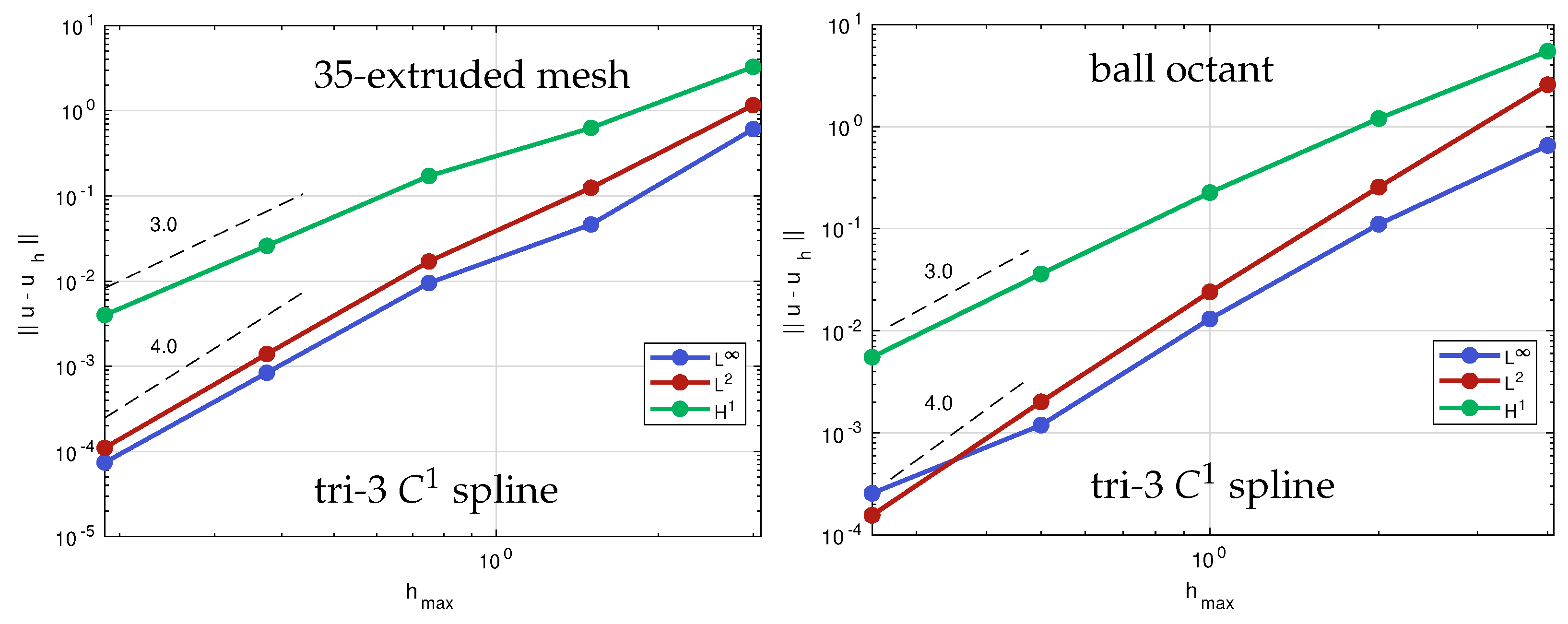
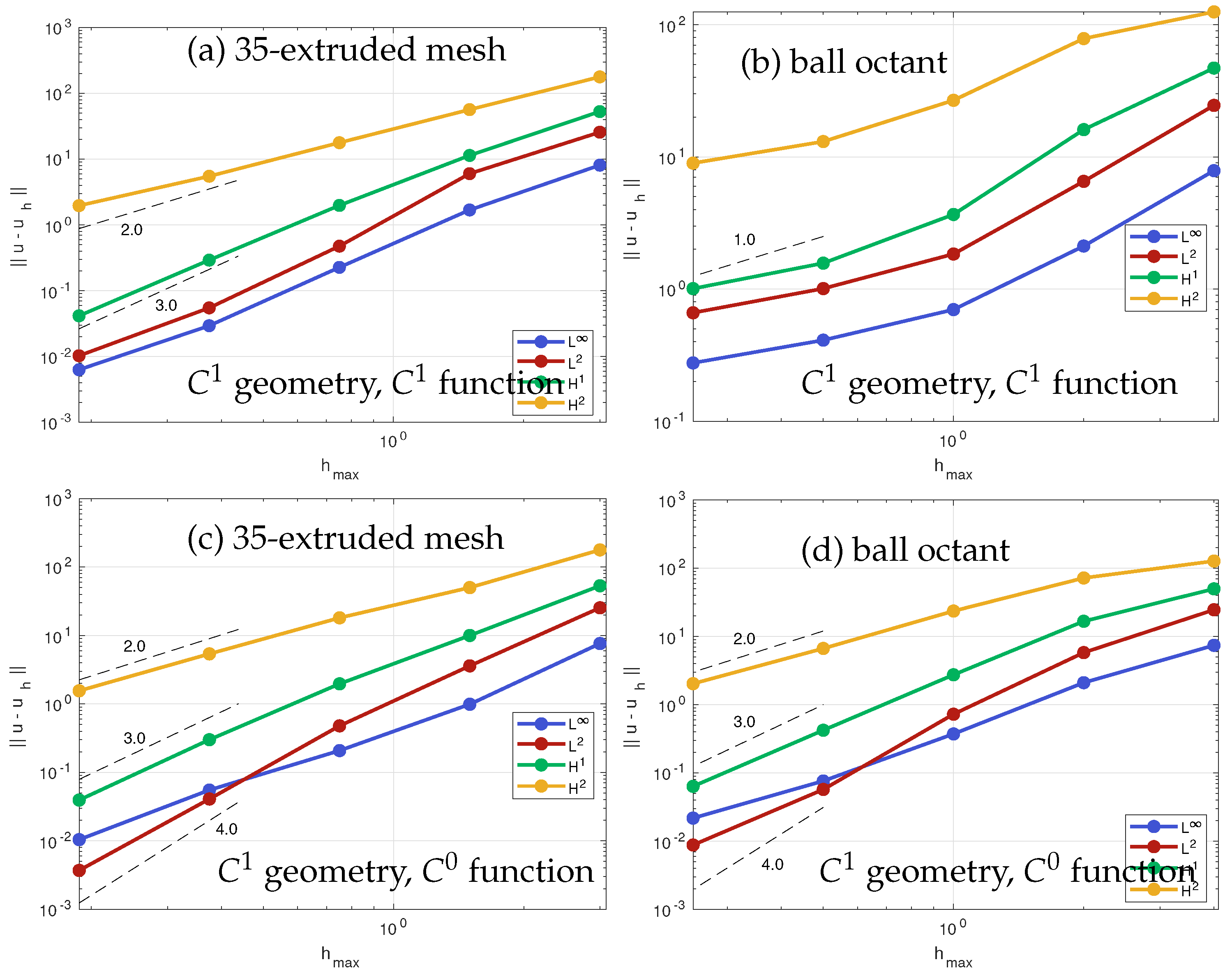
- a (fourth-order) convergence rate for Poisson’s equation on irregular box-complexes,
- i.e., the error between the computed and the known exact solution in the norm decreases by a factor of under halving of the mesh interval h, by in the error, and in the norm.
- for the regular case and for elements on geometry.
- convergence rate of singular tri-3 splines on singular tri-3 spline geometry is less than on irregular box-complexes.
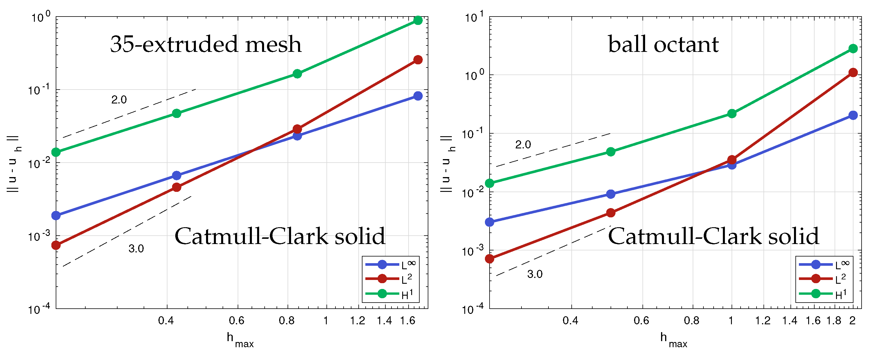
- in all cases enumerated above, tri-3 splines exhibit faster convergence than Catmull-Clark solids.
- Overview. After a brief literature review of trivariate smooth elements and the bivariate antecedents of tri-3 splines, Section 2 defines the tri-3 splines for unstructured box-complexes. The space is on regular local grids but is if initialized by knot insertion on a locally tensor-product grid. The space has zero first derivatives across irregularities but is after a change in variables and has linear-independent B-spline-like basis functions per box. Section 4 shows the numerical convergence for Poisson’s equation and compares the convergence to that of Catmull-Clark solids. Section 5 shows and discusses the convergence for the biharmonic equation and compares it to Catmull-Clark solids.
2. Smooth Trivariate Finite Elements
2.1. Singular Jet Collapse Constructions in Two Variables
2.2. Constructions in Three Variables
3. Tri-3 Splines on Unstructured Box-Complexes
- Notation and Indexing. Analogous to a simplicial complex, a box-complex (also known as a hex-mesh) in is a collection of d-dimensional boxes, , called d-boxes. Boxes of any dimension overlap only in complete lower-dimensional d-boxes. A 0-box is a vertex, a 1-box an edge, a 2-box a quadrilateral, and a 3-box is a quadrilateral-faced hexahedron. A box without a prefix is a 3-box.
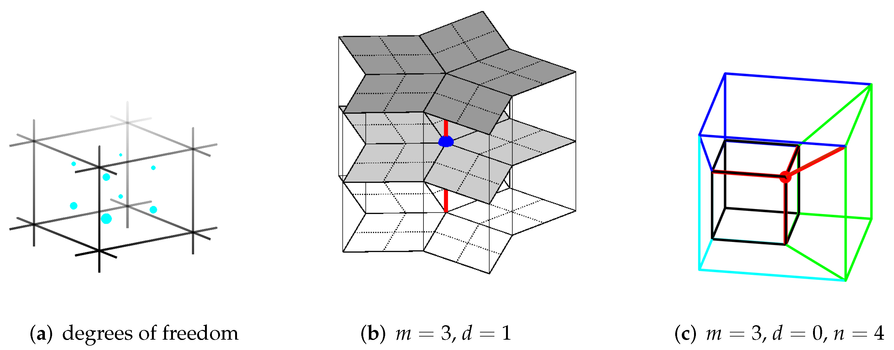
- Irregularities. For , an interior d-box is regular if it is completely surrounded by boxes and for , all incident -boxes are regular. For example, for a vertex to be regular, all edges incident to it must be regular. In , a regular vertex () is surrounded by 8 boxes, a regular edge () by 4 boxes, and a regular quadrilateral face () by 2 boxes. Interior faces are always regular since they are shared by exactly boxes.
- Polynomial pieces, corner inner, and index-wise nearest coefficients. A tri-3 spline consists of polynomial pieces represented in tri-variate tensor-product Bernstein-Bézier (BB) form (see [51] or [52]):where are the Bernstein-Bézier (BB) polynomials of degree 3 and, abbreviating , the row vectors are the BB-coefficients. De Casteljau’s algorithm can be used to evaluate the BB-form of Equation (1) and to re-express a polynomial on a subdomain of . Connecting to whenever is well-defined yields a mesh called the BB-net. Setting (or, symmetrically ) for exactly one leaves BB-coefficients that define restricted to a quad face of the domain cube. Setting for yields the BB-coefficients of a polynomial restricted to an edge in the direction , . The BB-coefficients with are called corner BB-coefficients since they are the values of in the domain corners . Two BB-coefficients and are index-wise nearest if there is no with in the -norm.
- The tri-3 splines. The splines are constructed by the following Algorithm 1.
Algorithm 1: Construction of tri-3 splines. Input: box-complex with vertices and values .Output: Tri-3 splines- Initialize the inner BB-coefficients , of each tri-3 piece by B-spline to BB-form conversion (knot insertion). In regular regions, the splines are, therefore, initially .
- Set the inner BB-coefficients of faces, the edges, and finally, the vertex as the average of their index-wise nearest neighbors.
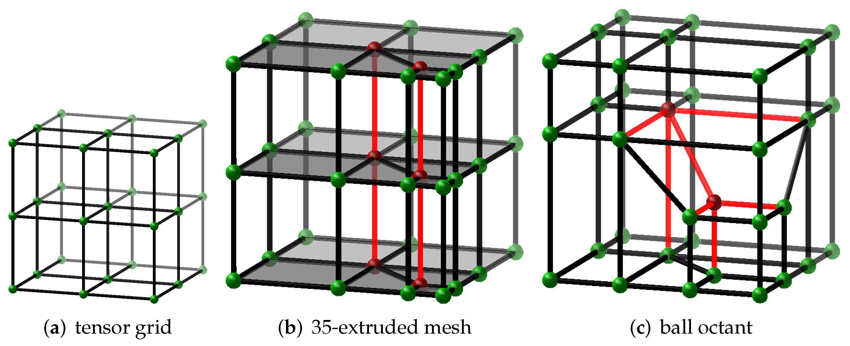
- For irregular boxes only, apply de Casteljau’s algorithm to split each tri-3 piece into pieces.
- For irregular sub-boxes apply the operator from Appendix A (cf. Section 6 of [11])
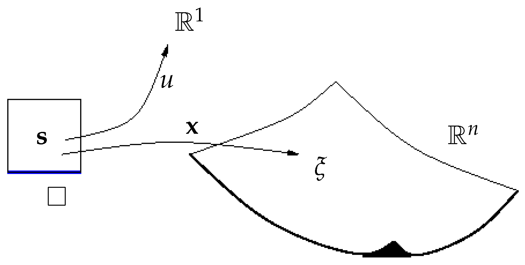
- The isogeometric approach. Let □ be a cube andbe the geometry map that defines the physical domain, see Figure 3. The function is to be determined so that satisfies the constraints, for example, as a solution to the Poisson equation or the biharmonic equation.
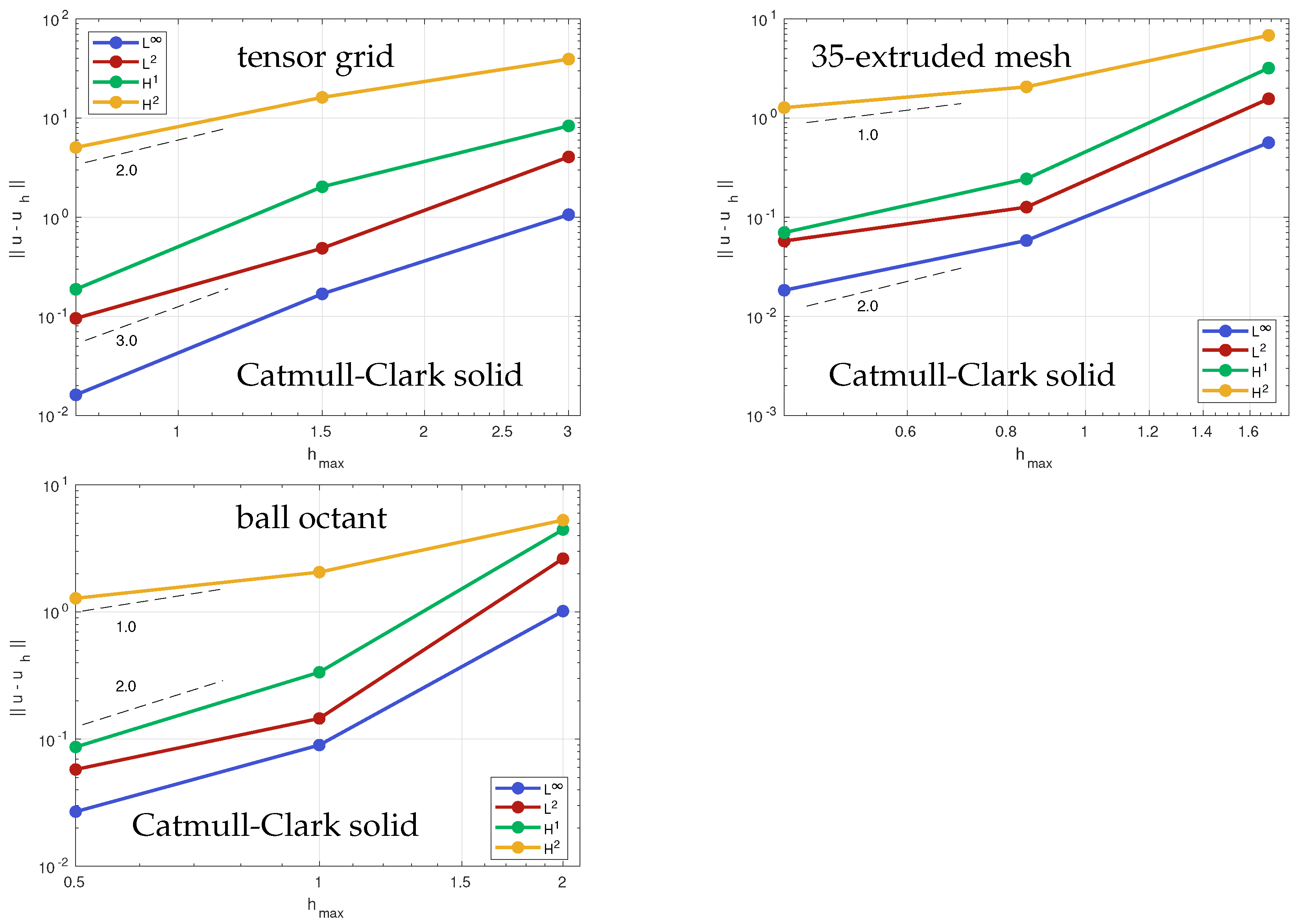
4. Solving Poisson’s Equation over Unstructured Hex Meshes
Comparison to Catmull-Clark Solids
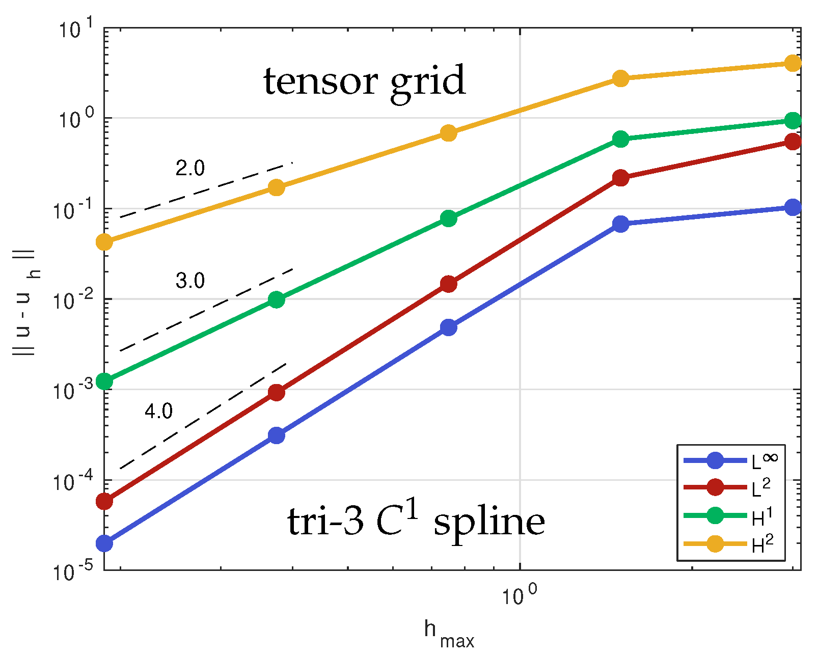
5. Solving the Biharmonic Equation over Unstructured Hex Meshes
6. Conclusions and Future Work
Author Contributions
Funding
Conflicts of Interest
Appendix A. Projector P
- 1.
- Compute a best-fit linear map ℓ to the BB-coefficients , , e.g., by computing a vector ℓ as
- 2.
- For each irregular sub-box , compute the polyhedral intersection by solving the systemwhere is the identity matrix, for and zero otherwise are the (local unit) labels of the three directions emanating from the irregular corner of , is the valence of the edge with label and, are the first two rows of , where is defined in (A5). Check that the system is well-conditioned, i.e., the sub-box is well-formed according to [11] (Def 2).
- 3.
- For each irregular sub-box , compute the BB-coefficients of the singular parameterization by
- 4.
- For each irregular sub-box , for ,For each inner BB-coefficient of a semi-regular edge of valence the bi-variate 2-neighborhood ‘orthogonal’ to the edge is transformed via , a jet collapse followed by projection. is applied to each coordinate of separately, generating defined byHere with the argument interpreted modulo .
- 5.
- For every face with BB-coefficients shared by an irregular sub-box and a (regular or irregular) sub-box , enforce regular continuity by averaging
References
- Walfisch, D.; Ryan, J.K.; Kirby, R.M.; Haimes, R. One-Sided Smoothness-Increasing Accuracy-Conserving Filtering for Enhanced Streamline Integration through Discontinuous Fields. J. Sci. Comput. 2009, 38, 164–184. [Google Scholar] [CrossRef] [Green Version]
- De Boor, C.; Höllig, K.; Riemenschneider, S. Box Splines; Springer: Berlin/Heidelberg, Germany, 1993. [Google Scholar]
- Peters, J.; Reif, U. Subdivision Surfaces. In Geometry and Computing; Springer: New York, NY, USA, 2008; Volume 3. [Google Scholar]
- Peters, J. Parametrizing singularly to enclose vertices by a smooth parametric surface. In Proceedings of the Graphics Interface ’91, Calgary, AB, Canada, 3–7 June 1991; pp. 1–7. [Google Scholar]
- Reif, U. TURBS—Topologically Unrestricted Rational B-Splines. Constr. Approx. 1998, 14, 57–77. [Google Scholar] [CrossRef]
- Nguyen, T.; Peters, J. Refinable C1 spline elements for irregular quad layout. Comput. Aided Geom. Des. 2016, 43, 123–130. [Google Scholar] [CrossRef] [Green Version]
- Toshniwal, D.; Speleers, H.; Hughes, T.J. Smooth cubic spline spaces on unstructured quadrilateral meshes with particular emphasis on extraordinary points: Geometric design and isogeometric analysis considerations. Comput. Methods Appl. Mech. Eng. 2017, 327, 411–458. [Google Scholar] [CrossRef]
- Duffy, M.G. Quadrature Over a Pyramid or Cube of Integrands with a Singularity at a Vertex. Siam J. Numer. Anal. 1982, 19, 1260–1262. [Google Scholar] [CrossRef]
- Karčiauskas, K.; Peters, J. Improved shape for refinable surfaces with singularly parameterized irregularities. Comput. Aided Des. 2017, 90, 191–198. [Google Scholar] [CrossRef] [Green Version]
- Wei, X.; Zhang, Y.J.; Toshniwal, D.; Speleers, H.; Li, X.; Manni, C.; Evans, J.A.; Hughes, T.J. Blended B-spline construction on unstructured quadrilateral and hexahedral meshes with optimal convergence rates in isogeometric analysis. Comput. Methods Appl. Mech. Eng. 2018, 341, 609–639. [Google Scholar] [CrossRef]
- Peters, J. Refinable tri-variate C1 splines for box-complexes including irregular points and irregular edges. Comput. Aided Geom. Des. 2020, 80, 1–21. [Google Scholar] [CrossRef]
- Braibant, V.; Fleury, C. Shape Optimal Design using B-splines. CMAME 1984, 44, 247–267. [Google Scholar] [CrossRef]
- Shyy, Y.; Fleury, C.; Izadpanah, K. Shape Optimal Design using higher-order elements. CMAME 1988, 71, 99–116. [Google Scholar]
- Au, F.; Cheung, Y. Isoparametric Spline Finite Strip for Plane Structures. Comput. Struct. 1993, 48, 22–32. [Google Scholar] [CrossRef]
- Schramm, U.; Pilkey, W.D. The coupling of geometric descriptions and finite elements using NURBS-A study in shape optimization. Finite Elem. Anal. Des. 1993, 340, 11–34. [Google Scholar] [CrossRef]
- Cirak, F.; Ortiz, M.; Schröder, P. Subdivision surfaces: A new paradigm for thin-shell finite-element analysis. Int. J. Numer. Methods Eng. 2000, 47, 2039–2072. [Google Scholar] [CrossRef]
- Hughes, T.J.R.; Cottrell, J.A.; Bazilevs, Y. Isogeometric Analysis: CAD, Finite Elements, NURBS, Exact Geometry and Mesh Refinement. Comput. Methods Appl. Mech. Eng. 2005, 194, 4135–4195. [Google Scholar] [CrossRef] [Green Version]
- Bazilevs, Y.; Beirao da Veiga, L.; Cottrell, J.A.; Hughes, T.J.; Sangalli, G. Isogeometric analysis: Approximation, stability and error estimates for h-refined meshes. Math. Model. Methods Appl. Sci. 2006, 16, 1031–1090. [Google Scholar] [CrossRef]
- Tagliabue, A.; Dede’, L.; Quarteroni, A. Isogeometric Analysis and error estimates for high order partial differential equations in Fluid Dynamics. Comput. Fluids 2014, 102, 277–303. [Google Scholar] [CrossRef]
- MacCracken, R.; Joy, K.I. Free-Form Deformations with Lattices of Arbitrary Topology. In Proceedings of the ACM Conference on Computer Graphics; ACM: New York, NY, USA, 1996; pp. 181–188. [Google Scholar]
- Burkhart, D.; Hamann, B.; Umlauf, G. Iso-geometric Finite Element Analysis Based on Catmull-Clark Subdivision Solids. Comput. Graph. Forum 2010, 29, 1575–1584. [Google Scholar] [CrossRef]
- de Boor, C. A Practical Guide to Splines; Springer: Berlin/Heidelberg, Germany, 1978. [Google Scholar]
- De Boor, C. B-form basics. In Geometric Modeling: Algorithms and New Trends; Farin, G., Ed.; SIAM: Philadelphia, PA, USA, 1987; pp. 131–148. [Google Scholar]
- Meyers, R.J.; Tautges, T.J. The “Hex-Tet” Hex-Dominant Meshing Algorithm as Implemented in CUBIT. In Itl. Meshing Roundtable; Freitag, L.A., Ed.; SIAM: Philadelphia, PA, USA, 1998; pp. 151–158. [Google Scholar]
- Mitchell, S.A. The All-Hex Geode-Template for Conforming a Diced Tetrahedral Mesh to any Diced Hexahedral Mesh. Eng. Comput. 1999, 15, 228–235. [Google Scholar] [CrossRef]
- Eppstein. Linear Complexity Hexahedral Mesh Generation. CGTA Comput. Geom. Theory Appl. 1999, 12, 58–67. [Google Scholar]
- Yamakawa, S.; Shimada, K. HEXHOOP: Modular Templates for Converting a Hex-Dominant Mesh to an ALL-Hex Mesh. Eng. Comput. 2002, 18, 211–228. [Google Scholar] [CrossRef] [Green Version]
- Gregson, J.; Sheffer, A.; Zhang, E. All-Hex Mesh Generation via Volumetric PolyCube Deformation. Comput. Graph. Forum 2011, 30, 1407–1416. [Google Scholar] [CrossRef] [Green Version]
- Johnen, A.; Weill, J.C.; Remacle, J.F. Robust and efficient validation of the linear hexahedral element. Procedia Eng. 2017, 203, 271–283. [Google Scholar] [CrossRef]
- Owen, S.J.; Brown, J.A.; Ernst, C.D.; Lim, H.; Long, K.N. Hexahedral Mesh Generation for Computational Materials Modeling. Procedia Eng. 2017, 203, 167–179. [Google Scholar] [CrossRef]
- Nieser, M.; Reitebuch, U.; Polthier, K. Section 2: Cube Cover—Parameterization of 3D Volumes. Comput. Graph. Forum 2011, 30, 1397–1406. [Google Scholar] [CrossRef]
- Liu, H.; Zhang, P.; Chien, E.; Solomon, J.; Bommes, D. Singularity-constrained octahedral fields for hexahedral meshing. ACM Trans. Graph 2018, 37, 93:1–93:17. [Google Scholar] [CrossRef]
- DeRose, T. Necessary and sufficient conditions for tangent plane continuity of Bézier surfaces. Comput. Aided Geom. Des. 1990, 7, 165–180. [Google Scholar] [CrossRef]
- Peters, J. Geometric Continuity. Handbook of Computer Aided Geometric Design; Elsevier: Amsterdam, The Netherlands, 2002; pp. 193–229. [Google Scholar]
- Birner, K.; Jüttler, B.; Mantzaflaris, A. Bases and dimensions of C1-smooth isogeometric splines on volumetric two-patch domains. Graph. Model. 2018, 99, 46–56. [Google Scholar] [CrossRef] [Green Version]
- Birner, K.; Kapl, M. The space of C1-smooth isogeometric spline functions on trilinearly parameterized volumetric two-patch domains. Comput. Aided Geom. Des. 2019, 70, 16–30. [Google Scholar] [CrossRef]
- Kapl, M.; Vitrih, V. C1 isogeometric spline space for trilinearly parameterized multi-patch volumes. Comput. Math. Appl. 2022, 117, 53–68. [Google Scholar] [CrossRef]
- Catmull, E.; Clark, J. Recursively generated B-spline surfaces on arbitrary topological meshes. Comput.-Aided Des. 1978, 10, 350–355. [Google Scholar] [CrossRef]
- Doo, D.; Sabin, M. Behaviour of recursive division surfaces near extraordinary points. Comput.-Aided Des. 1978, 10, 356–360. [Google Scholar] [CrossRef]
- Altenhofen, C.; Ewald, T.; Stork, A.; Fellner, D. Analyzing and Improving the Parametrization Quality of Catmull-Clark Solids for Isogeometric Analysis. IEEE Comput. Graph. Appl. 2021, 41, 34–47. [Google Scholar] [CrossRef]
- Xie, J.; Xu, J.; Dong, Z.; Xu, G.; Deng, C.; Mourrain, B.; Zhang, Y.J. Interpolatory Catmull-Clark volumetric subdivision over unstructured hexahedral meshes for modeling and simulation applications. Comput. Aided Geom. Des. 2020, 80, 101867. [Google Scholar] [CrossRef]
- Höllig, K.; Reif, U.; Wipper, J. Weighted Extended B-Spline Approximation of Dirichlet Problems. SIAM Numer. Anal. 2001, 39, 442–462. [Google Scholar] [CrossRef]
- Buhmann, M.D. Radial Basis Functions-Theory and Implementations; Cambridge Monographs on Applied and Computational Mathematics; Cambridge University Press: London, UK, 2009; Volume 12, pp. 1–259. [Google Scholar]
- Nitsche, J. Über ein Variationsprinzip zur Lösung von Dirichlet-Problemen bei Verwendung von Teilräumen, die keinen Randbedingungen unterworfen sind. In Abhandlungen aus dem Mathematischen Seminar der Universität Hamburg; Springer: Berlin/Heidelberg, Germany, 1971; Volume 36, pp. 9–15. [Google Scholar]
- Pfluger, P.R.; Neamtu, M. On degenerate surface patches. Numer. Algorithms 1993, 5, 569–575. [Google Scholar] [CrossRef]
- Neamtu, M.; Pfluger, P.R. Degenerate polynomial patches of degree 4 and 5 used for geometrically smooth interpolation in 3. Comput. Aided Geom. Des. 1994, 11, 451–474. [Google Scholar] [CrossRef]
- Reif, U. A refinable space of smooth spline surfaces of arbitrary topological genus. J. Approx. Theory 1997, 90, 174–199. [Google Scholar] [CrossRef] [Green Version]
- Bohl, H.; Reif, U. Degenerate Bézier patches with continuous curvature. Comput. Aided Geom. Des. 1997, 14, 749–761. [Google Scholar] [CrossRef]
- Peters, J. Smooth interpolation of a mesh of curves. Constr. Approx. 1991, 7, 221–247. [Google Scholar] [CrossRef]
- Kang, H.; Xu, J.; Chen, F.; Deng, J. A new basis for PHT-splines. Graph. Model. 2015, 82, 149–159. [Google Scholar] [CrossRef]
- Farin, G. Curves and Surfaces for Computer Aided Geometric Design: A Practical Guide; Academic Press: San Diego, CA, USA, 2002. [Google Scholar]
- Prautzsch, H.; Boehm, W.; Paluszny, M. Bézier and B-Spline Techniques; Springer: Berlin/Heidelberg, Germany, 2002. [Google Scholar]
- Wei, X.; Zhang, Y.J.; Hughes, T.J.R. Truncated hierarchical tricubic spline construction on unstructured hexahedral meshes for isogeometric analysis applications. Comput. Math. Appl. 2017, 74, 2203–2220. [Google Scholar] [CrossRef]
- Elman, H.; Silvexter, D.; Wathen, A. Finite Elements and Fast Iterative Solvers: With Applications in Incompressible Fluid Dynamics; Oxford Scholarship Online: Oxford, UK, 2014. [Google Scholar]
- Kremer, M.; Bommes, D.; Kobbelt, L. OpenVolumeMesh-A Versatile Index-Based Data Structure for 3D Polytopal Complexes. In Proceedings of the 21st International Meshing Roundtable, San Jose, CA, USA, 7–10 October 2012; Springer: San Jose, CA, USA, 2012; pp. 531–548. [Google Scholar]
- Pan, Q.; Xu, G.; Xu, G.; Zhang, Y. Isogeometric analysis based on extended Catmull–Clark subdivision. Comput. Math. Appl. 2016, 71, 105–119. [Google Scholar] [CrossRef]
- Liu, Z.; McBride, A.T.; Saxena, P.; Steinmann, P. Assessment of an isogeometric approach with Catmull–Clark subdivision surfaces using the Laplace–Beltrami problems. Comput. Mech. 2020, 66, 851–876. [Google Scholar] [CrossRef]
- Ciarlet, P.G.; Raviart, P.A. A mixed finite element method for the biharmonic equation. In Mathematical Aspects of Finite Elements in Partial Differential Equations; Academic Press: Amsterdam, The Netherlands, 1974; pp. 125–145. [Google Scholar]
- Falk, R.S. Approximation of the biharmonic equation by a mixed finite element method. Siam J. Numer. Anal. 1978, 15, 556–567. [Google Scholar] [CrossRef]
- Arnold, D.N.; Brezzi, F. Mixed and nonconforming finite element methods: Implementation, postprocessing and error estimates. Esaim Math. Model. Numer. Anal. 1985, 19, 7–32. [Google Scholar] [CrossRef] [Green Version]
- Pan, K.; He, D.; Ni, R. An efficient multigrid solver for 3D biharmonic equation with a discretization by 25-point difference scheme. arXiv 2019, arXiv:1901.05118. [Google Scholar]
- Gómez, H.; Calo, V.M.; Bazilevs, Y.; Hughes, T.J. Isogeometric analysis of the Cahn–Hilliard phase-field model. Comput. Methods Appl. Mech. Eng. 2008, 197, 4333–4352. [Google Scholar] [CrossRef]
- Wang, W.; Zhang, Y.; Liu, L.; Hughes, T.J. Trivariate solid T-spline construction from boundary triangulations with arbitrary genus topology. Comput.-Aided Des. 2013, 45, 351–360. [Google Scholar] [CrossRef]
- Wang, W.; Zhang, Y.; Xu, G.; Hughes, T.J. Converting an unstructured quadrilateral/hexahedral mesh to a rational T-spline. Comput. Mech. 2012, 50, 65–84. [Google Scholar] [CrossRef]
- Wells, G.N.; Kuhl, E.; Garikipati, K. A discontinuous Galerkin method for the Cahn–Hilliard equation. J. Comput. Phys. 2006, 218, 860–877. [Google Scholar] [CrossRef]
- Xia, Y.; Xu, Y.; Shu, C.W. Local discontinuous Galerkin methods for the Cahn–Hilliard type equations. J. Comput. Phys. 2007, 227, 472–491. [Google Scholar] [CrossRef]
- Mu, L.; Wang, J.; Ye, X. Weak Galerkin finite element methods for the biharmonic equation on polytopal meshes. Numer. Methods Partial Differ. Equ. 2014, 30, 1003–1029. [Google Scholar] [CrossRef] [Green Version]
- Koh, K.J.; Toshniwal, D.; Cirak, F. An optimally convergent smooth blended B-spline construction for semi-structured quadrilateral and hexahedral meshes. Comput. Methods Appl. Mech. Eng. 2022, 399, 115438. [Google Scholar] [CrossRef]


Publisher’s Note: MDPI stays neutral with regard to jurisdictional claims in published maps and institutional affiliations. |
© 2022 by the authors. Licensee MDPI, Basel, Switzerland. This article is an open access article distributed under the terms and conditions of the Creative Commons Attribution (CC BY) license (https://creativecommons.org/licenses/by/4.0/).
Share and Cite
Youngquist, J.; Peters, J. Solving Biharmonic Equations with Tri-Cubic C1 Splines on Unstructured Hex Meshes. Axioms 2022, 11, 633. https://doi.org/10.3390/axioms11110633
Youngquist J, Peters J. Solving Biharmonic Equations with Tri-Cubic C1 Splines on Unstructured Hex Meshes. Axioms. 2022; 11(11):633. https://doi.org/10.3390/axioms11110633
Chicago/Turabian StyleYoungquist, Jeremy, and Jörg Peters. 2022. "Solving Biharmonic Equations with Tri-Cubic C1 Splines on Unstructured Hex Meshes" Axioms 11, no. 11: 633. https://doi.org/10.3390/axioms11110633