
A Probe into a (2 + 1)-Dimensional Combined Cosmological Model in f(R, T) Gravity


Abstract
:1. Introduction
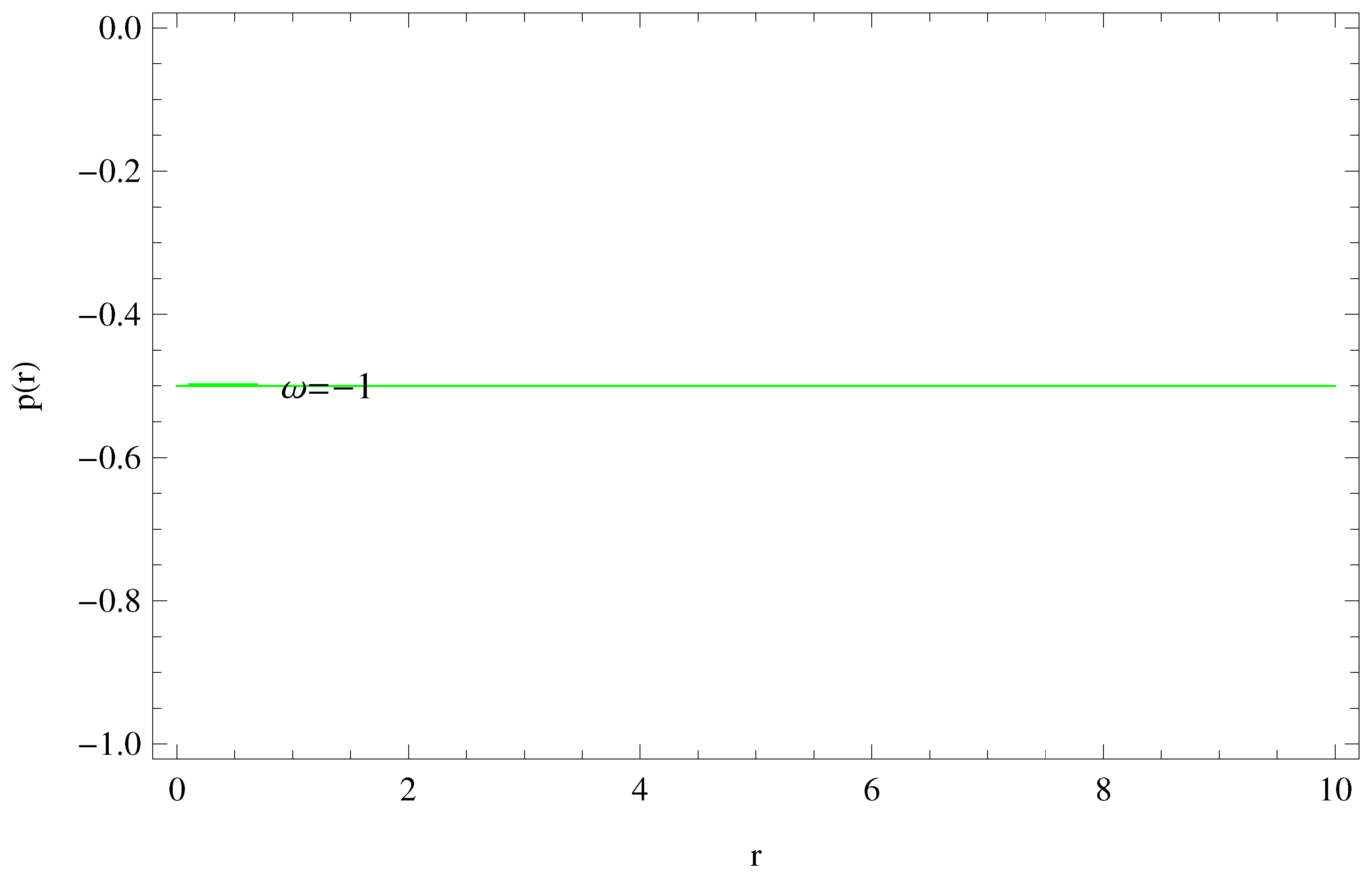
2. Exploring New Solutions under Models
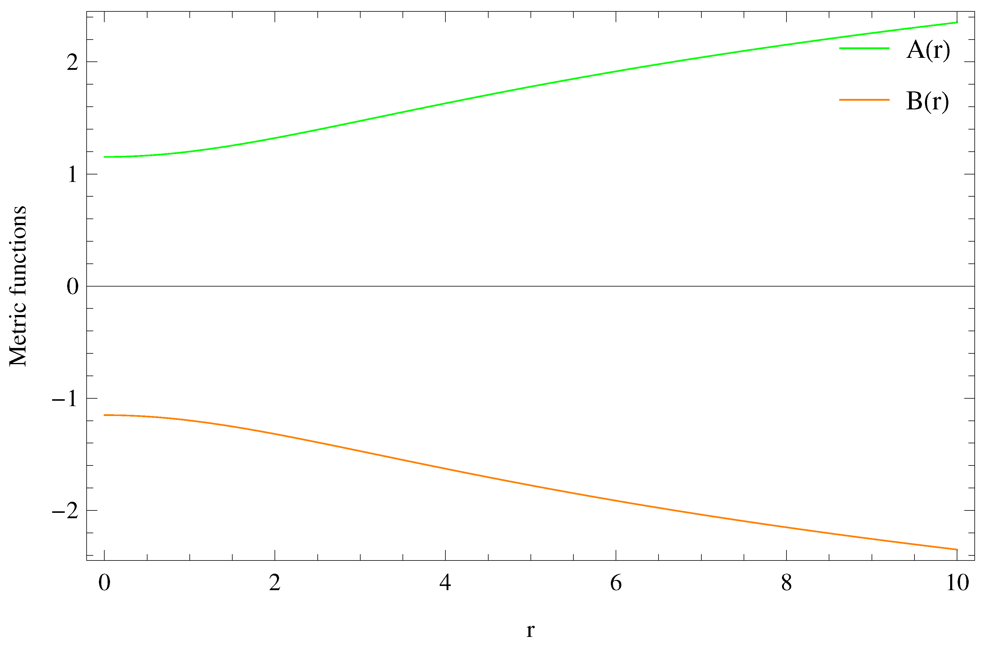
3. (2+1)-Dimensional Spacetime Metric
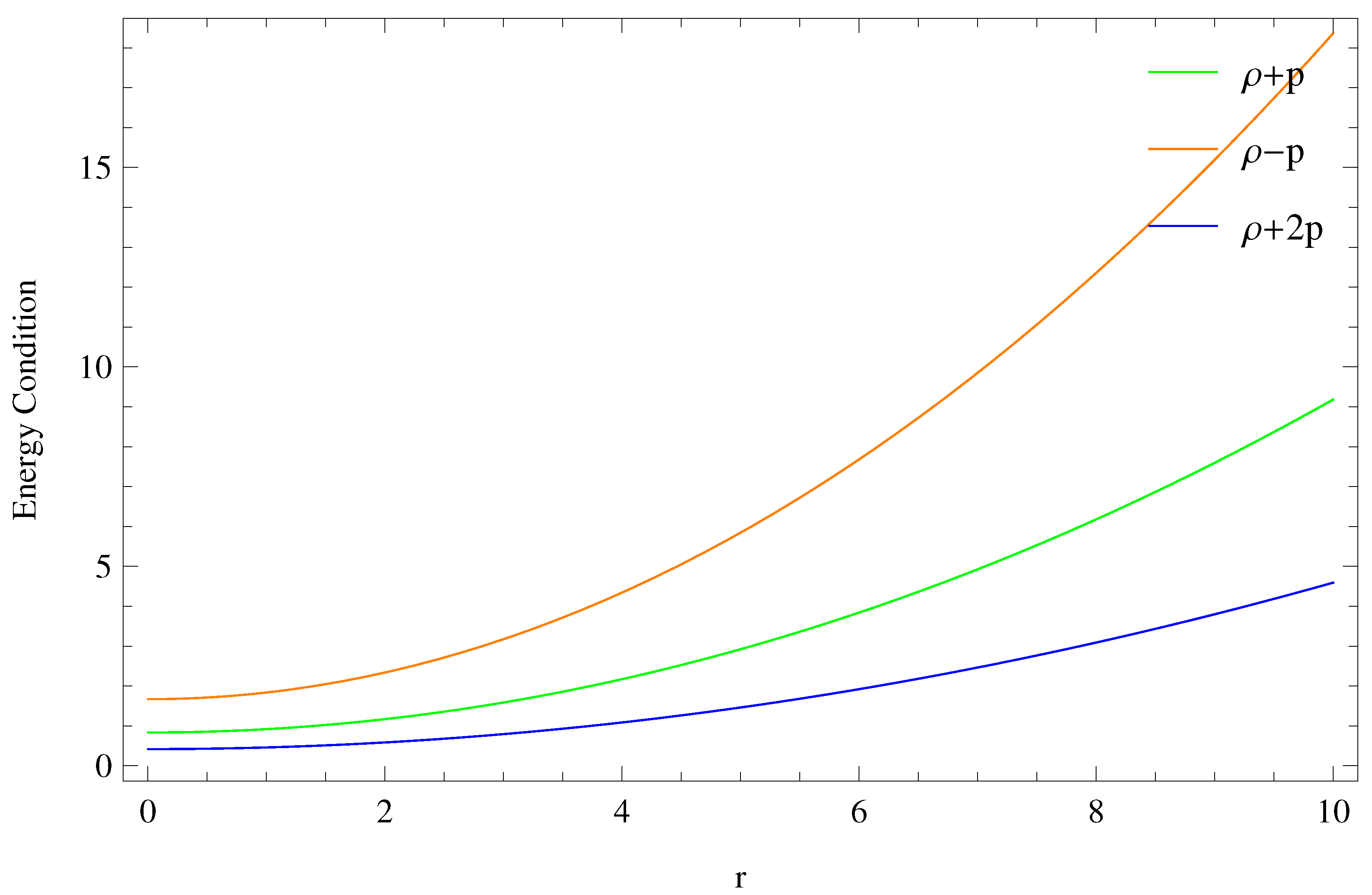
- (i)
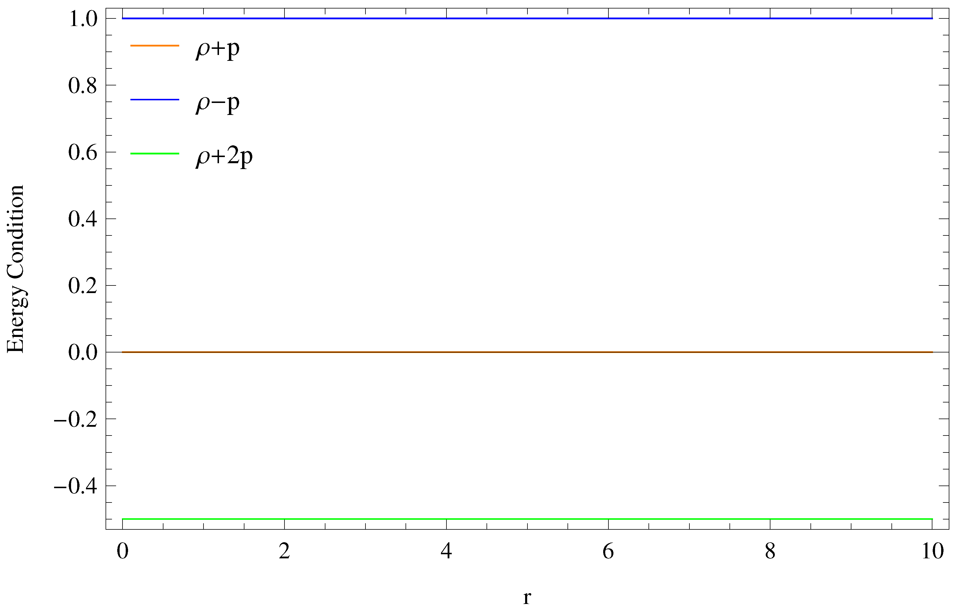
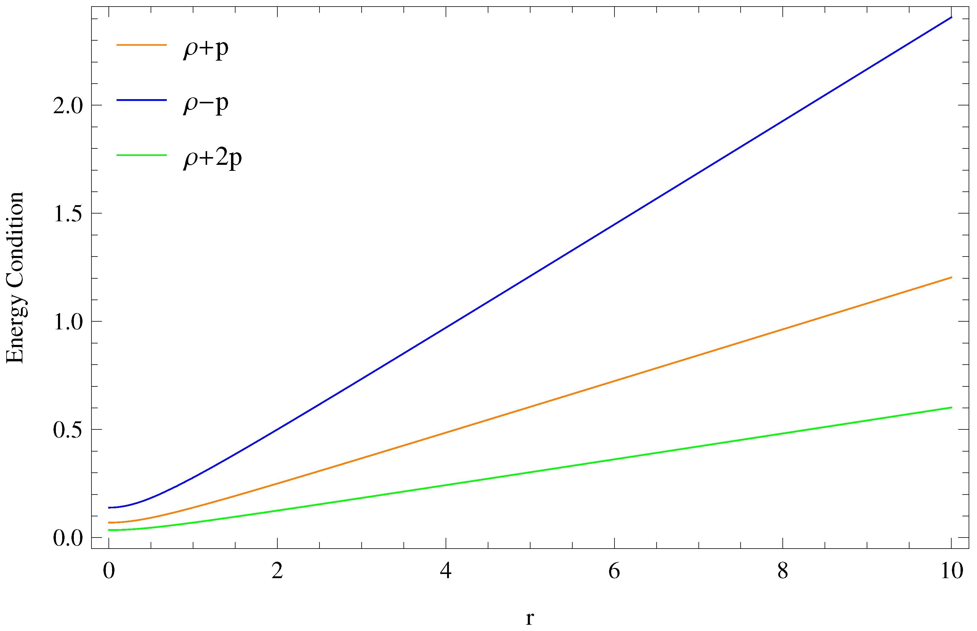
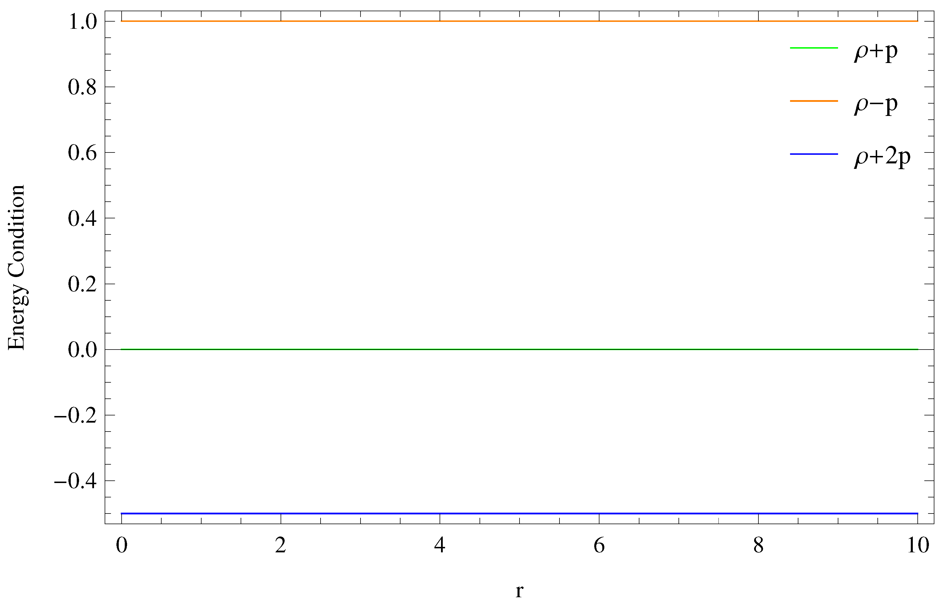
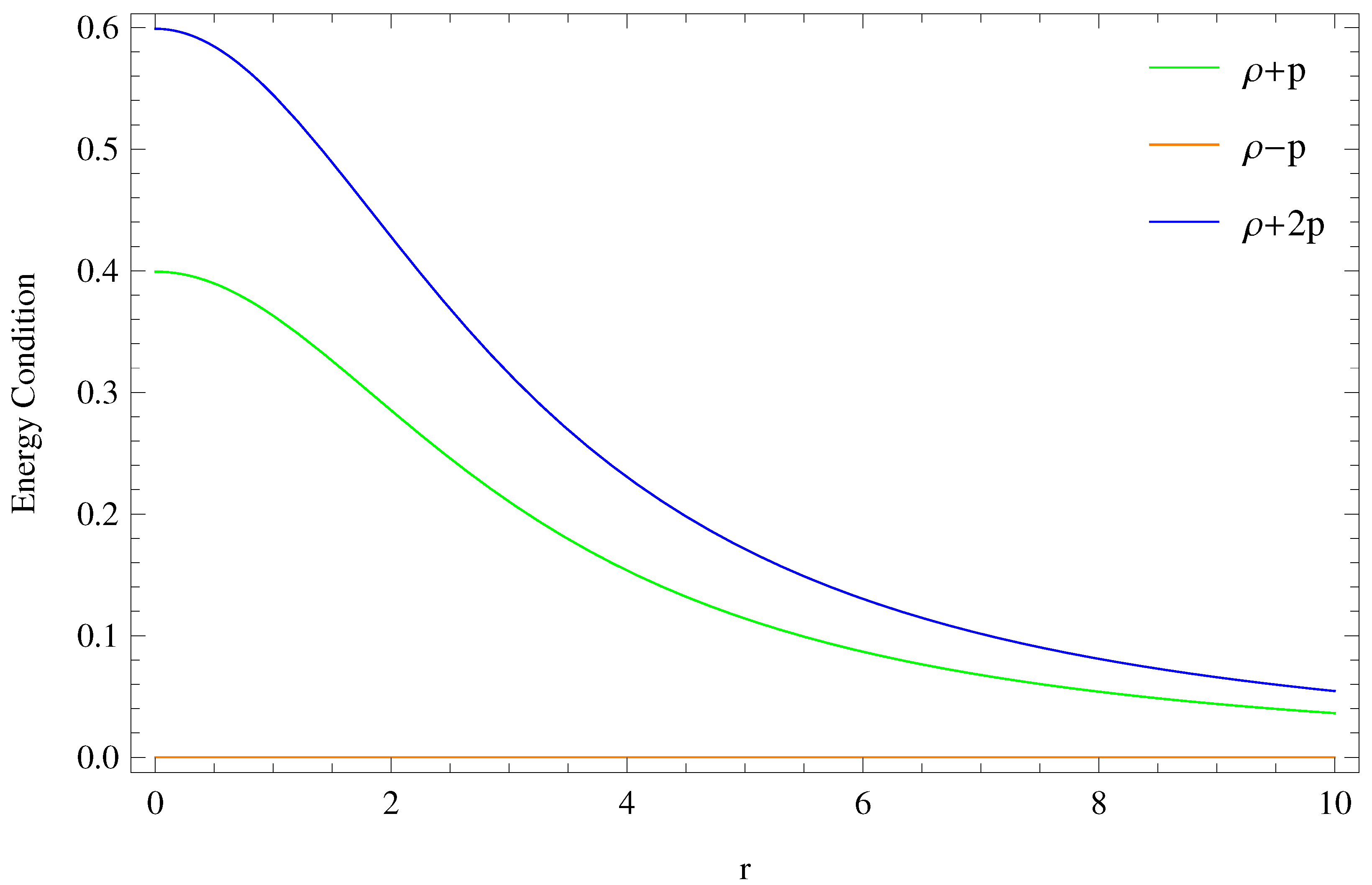
- Null energy condition or NEC: ,
- (ii)
- Weak energy condition or WEC: , ,
- (iii)
- Dominant energy condition or DEC: ,
- (iv)
- Strong energy condition or SEC: , .
4. Effective Mass and Redshift Function
5. Concluding Remarks
Author Contributions
Funding
Acknowledgments
Conflicts of Interest
References
- Gao, C.; Wu, F.; Chen, X. Holographic dark energy model from Ricci scalar curvature. Phys. Rev. D 2009, 79, 043511. [Google Scholar] [CrossRef] [Green Version]
- Capozziello, S.; Moruno, P.M.; Rubano, C. Dark energy and dust matter phases from an exact f(R)-cosmology model. Phys. Lett. B 2008, 664, 12. [Google Scholar] [CrossRef] [Green Version]
- Capozziello, S.; Cardone, V.F.; Troisi, A. Dark energy and dark matter as curvature effects? New Astron. Rev. 2007, 51, 341. [Google Scholar] [CrossRef]
- B<i>o</i>¨hmer, C.G.; Fodor, G. Perfect Fluid Spheres with Cosmological Constant. Phys. Rev. D 2008, 77, 064008. [Google Scholar]
- Banados, M.; Teitelboim, C.; Zanelli, J. Black hole in three-dimensional spacetime. Phys. Rev. Lett. 1992, 69, 1849–1851. [Google Scholar]
- Gibbons, G.; Hawking, S. Action integrals and partition functions in quantum gravity. Phy. Rev. D 1997, 15, 2752. [Google Scholar] [CrossRef]
- Carlip, S. Observables, gauge invariance, and time in (2+1)-dimensional quantum gravity. Phys. Rev. D 1990, 42, 2647. [Google Scholar] [CrossRef]
- Ba<i>n</i>˜ados, M.; Henneaux, M.; Teitelboim, C.; Zanelli, J. Geometry of the (2+1) black hole. Phys. Rev. D 1993, 48, 1506–1525. [Google Scholar]
- Kamata, M.; Koikawa, T. The electrically charged BTZ black hole with self (anti-self) dual Maxwell field. Phys. Lett. B 1995, 353, 196–200. [Google Scholar] [CrossRef] [Green Version]
- Banados, M.; Brotz, T.; Ortiz, M. Boundary dynamics and the statistical mechanics of the 2+1-dimensional black hole. Nucl. Phys. B 1999, 545, 340–370. [Google Scholar] [CrossRef] [Green Version]
- Oliva, J.; Tempo, D.; Troncoso, R. Three-dimensional black holes, gravitational solitons, kinks and wormholes for BHT massive gravity. J. High Energy Phys. 2009, 2009, 011. [Google Scholar] [CrossRef] [Green Version]
- Alkac, G.; Kilicarslan, E.; Tekin, B. Asymptotically flat black holes in 2+1 dimensions. Phys. Rev. D 2016, 93, 084003. [Google Scholar] [CrossRef] [Green Version]
- Koch, B.; Reyes, I.A.; Rincon, A. A scale dependent black hole in three-dimensional space-time. Class. Quantum Gravity 2016, 33, 22. [Google Scholar] [CrossRef]
- Panotopoulos, G.; Rincon, A. Greybody factors for a nonminimally coupled scalar field in BTZ black hole background. Phys. Lett. B 2017, 772, 523–528. [Google Scholar] [CrossRef]
- Afshar, H.; Grumiller, D.; Merbis, W.; Pérez, A.; Tempo, D.; Troncoso, R. Soft hairy horizons in three spacetime dimensions. Phys. Rev. D 2017, 95, 106005. [Google Scholar] [CrossRef] [Green Version]
- Rincon, A.; Koch, B. Scale-dependent rotating BTZ black hole. Eur. Phys. J. C 2018, 78, 1022. [Google Scholar] [CrossRef]
- Oliveira-Neto, G. Scalar Field Cosmology in Three-Dimensions. Bras. J. Phys. 2001, 31, 456–460. [Google Scholar] [CrossRef]
- Barrow, J.D.; Shaw, D.J.; Tsagas, C.G. Cosmology in three dimensions: Steps towards the general solution. Class. Quant. Grav. 2006, 23, 5291–5322. [Google Scholar] [CrossRef]
- Pavluchenko, S.A. Cosmological dynamics of spatially flat Einstein-Gauss-Bonnet models in various dimensions. Vacuum case. Phys. Rev. D 2016, 94, 084019. [Google Scholar] [CrossRef] [Green Version]
- Pavluchenko, S.A. Dynamics of the cosmological models with perfect fluidin Einstein-Gauss-Bonnet gravity: Low-dimensional case. Eur. Phys. J. C 2019, 79, 111. [Google Scholar] [CrossRef] [Green Version]
- Felisola, O.C.; Orellana, O.; Perdiguero, I.; Ramírez, F.; Skirzewski, A.; Zerwekh, A.R. Aspects of the polynomial affine model of gravity in three dimensions. Eur. Phys. J. C 2022, 82, 8. [Google Scholar] [CrossRef]
- Overduin, J.M.; Cooperstock, F.I. Evolution of the scale factor with a variable cosmological term. Phys. Rev. D 1998, 58, 043506. [Google Scholar] [CrossRef] [Green Version]
- Hammad, F. A note on the effect of the cosmological constant on the bending of light. Mod. Phys. Lett. A 2013, 28, 1350181. [Google Scholar] [CrossRef]
- Bonanno, A.; Carloni, S. Dynamical system analysis of cosmologies with running cosmological constant from quantum Einstein gravity. New J. Phys. 2012, 14, 025008. [Google Scholar] [CrossRef] [Green Version]
- Anagnostopoulos, F.K.; Bonanno, A.; Mitra, A.; Zarikas, V. A Swiss-cheese cosmologies with variable G and λ from the renormalization group. Phys. Rev. D 2022, 105, 8. [Google Scholar] [CrossRef]
- Reuter, M.; Saueressig, F. Nonlocal quantum gravity and the size of the universe. Prog. Phys. 2004, 52, 6–7. [Google Scholar] [CrossRef] [Green Version]
- Alvarez, P.D.; Koch, B.; Laporte, C.; Rincón, A. Can scale-dependent cosmology alleviate the H0 tension? J. Cosmol. Astropart. Phys. 2021, 2021, 019. [Google Scholar] [CrossRef]
- Sola, P.J. Cosmological constant and vacuum energy: Old and new ideas. J. Phys. Conf. Ser. 2013, 453, 012015. [Google Scholar]
- Chen, W.; Wu, Y.S. Implications of a cosmological constant varying as R-2. Phys. Rev. D 1990, 41, 695, Erratum Phys. Rev. D 1992, 45, 4728. [Google Scholar] [CrossRef]
- Izawa, K. Dynamics of the Cosmological Constant in Two-Dimensional Universe. Prog. Theor. Phys. 1994, 91, 2. [Google Scholar] [CrossRef]
- Singh, V.; Singh, C.P. Modified f(R, T) gravity theory and scalar field cosmology. Astrophys. Space Sci. 2015, 356, 153. [Google Scholar] [CrossRef]
- Harko, T. f(R, T) gravity. Phys. Rev. D 2011, 84, 024020. [Google Scholar] [CrossRef] [Green Version]
- Pawar, D.D.; Dagwal, V.J. Cosmological models in f(R, T) theory of gravitation. Aryabhatta J. Math. Inform. 2015, 7, 17. [Google Scholar]
- Houndjo, M.J.S.; Batista, C.E.M.; Campos, J.P.; Piattella, O.F. Finite-time singularities in f(R, T) gravity and the effect of conformal anomaly. Can. J. Phys. 2013, 91, 548. [Google Scholar] [CrossRef] [Green Version]
- Islam, S.; Kumar, P.; Khadekar, G.S.; Das, T.K. (2+1) dimensional cosmological models in f(R, T) gravity with Λ(R, T). IOP Conf. Ser. J. Phys. Conf. Ser. 2019, 1258, 012026. [Google Scholar] [CrossRef]
- Cornish, N.J.; Frankel, N.E. Gravitation in 2+1 dimensions. Phys. Rev. D 1991, 43, 8. [Google Scholar] [CrossRef]
- Ahmed, N.; Pradhan, A.; Fekry, M.; Alamri, S.Z. V cosmological models in modified gravity with by using generation technique. NRIAG J. Astron. Geophys. 2016, 5, 35–47. [Google Scholar] [CrossRef] [Green Version]
- Padmanabhan, T. Cosmological constant-the weight of the vacuum. Phys. Rep. 2003, 380, 235–320. [Google Scholar] [CrossRef] [Green Version]
- Rahaman, F.; Bhar, P.; Biswas, R.; Usmani, A.A. Exact interior solutions in 2+1-dimensional spacetime. Eur. Phys. J. C 2014, 74, 2845. [Google Scholar] [CrossRef] [Green Version]
- Caldwell, R.R.; Dave, R.; Steinhardt, P.J. Cosmological Imprint of an Energy Component with General Equation of State. Phys. Rev. Lett. 1988, 80, 1582–1585. [Google Scholar] [CrossRef] [Green Version]
- Qian, Z. Ricci flow on a 3-manifold with positive scalar curvature. Bull. Sci. Math. 2009, 133, 145–168. [Google Scholar] [CrossRef] [Green Version]
- Kim, J.R. Relative Lorentzian volume comparison with integral Ricci and scalar curvature bound. J. Geom. Phys. 2011, 61, 1061–1069. [Google Scholar] [CrossRef]
- Eisenhart, L.P. Spaces for which the Ricci scalar R is equal to zero. Proc. Natl. Acad. Sci. USA 1958, 44, 695–698. [Google Scholar] [CrossRef] [PubMed] [Green Version]
- Kawakami, H. On some pasting cylinders onto a manifold with negative (Ricci, scalar) curvature along compact boundaries. Tsukuba J. Math. 1990, 14, 413–421. [Google Scholar] [CrossRef]
- Rahaman, F.; Usmani, A.A.; Ray, S.; Islam, S. The (2+1)-dimensional charged gravastars. Phys. Lett. B 2012, 707, 319. [Google Scholar] [CrossRef]
- Oesch, P.A.; Brammer, G.; Dokkum, V.P. A remarkably luminous galaxy at Z = 11.1 measured with hubble space telescope grism spectroscopy. Astrophys. J. 2016, 819, 129. [Google Scholar] [CrossRef] [Green Version]
- Curiel, E. A Primer on Energy conditions. arXiv 2014, arXiv:1405.0403. [Google Scholar]
- Farnes, J.S. A Unifying Theory of Dark Energy and Dark Matter: Negative Masses and Matter Creation within a Modified ΛCDM Framework. Astron. Astrophys. 2018, 620, A92. [Google Scholar] [CrossRef] [Green Version]
- Visser, M.; Barcelo, C. Energy Conditions and Their Cosmological Implications. arXiv 2000, arXiv:gr-qc/0001099. [Google Scholar] [CrossRef]
- Stephani, H.; Kramer, D.; MacCallum, M.; Hoenselaers, C.; Herlt, E. Exact Solutions of Einstein’s Field Equations, 2nd ed.; Cambridge University Press: Cambridge, UK, 2003. [Google Scholar]


Publisher’s Note: MDPI stays neutral with regard to jurisdictional claims in published maps and institutional affiliations. |
© 2022 by the authors. Licensee MDPI, Basel, Switzerland. This article is an open access article distributed under the terms and conditions of the Creative Commons Attribution (CC BY) license (https://creativecommons.org/licenses/by/4.0/).
Share and Cite
Islam, S.; Aamir, M.; Radinschi, I.; Bandyopadhyay, D. A Probe into a (2 + 1)-Dimensional Combined Cosmological Model in f(R, T) Gravity. Axioms 2022, 11, 605. https://doi.org/10.3390/axioms11110605
Islam S, Aamir M, Radinschi I, Bandyopadhyay D. A Probe into a (2 + 1)-Dimensional Combined Cosmological Model in f(R, T) Gravity. Axioms. 2022; 11(11):605. https://doi.org/10.3390/axioms11110605
Chicago/Turabian StyleIslam, Safiqul, Muhammad Aamir, Irina Radinschi, and Dwiptendra Bandyopadhyay. 2022. "A Probe into a (2 + 1)-Dimensional Combined Cosmological Model in f(R, T) Gravity" Axioms 11, no. 11: 605. https://doi.org/10.3390/axioms11110605