Enhanced Lot Acceptance Testing Based on Defect Counts and Posterior Odds Ratios

Abstract

Optimal defects-per-unit test plans based on posterior odds ratios are developed for the disposition of product lots. The number of nonconformities per unit is modeled by the Conway–Maxwell–Poisson distribution rather than the typical Poisson model. In essence, a submitted batch is conforming if its posterior acceptability is sufficiently large. First, a useful approximation of the optimal test plan is derived in closed form using the asymptotic normality of the log ratio. A mixed-integer nonlinear programming problem is then solved via Monte Carlo simulation to find the smallest number of inspected items per lot and the maximum tolerable posterior odds ratio. The methodology is applied to the manufacturing of paper and glass. The suggested sampling plan for lot sentencing provides the specified protections to both manufacturers and customers and minimizes the needed sample size. In terms of inspection effort and accuracy, the proposed approach is virtually an advantageous extension of the classical frequentist perspective. In many practical cases, it yields more precise assessments of the current consumer and producer risks, as well as more realistic decision rules.

1. Introduction

Sampling inspection plans for lot acceptance are often designed in industry to suitably discriminate between satisfactory and unsatisfactory batches. In essence, the construction of the best decision rule for lot disposition can be stated as a constrained optimization problem. Generally, proper acceptance test plans must provide the desired protections to both customers and manufacturers, and the required number of items to be sampled should be as small as possible. Many test plans are available in the literature for sentencing lots of incoming or outgoing goods. Papers [1,2,3,4,5,6,7,8,9,10,11,12,13,14] are just a sample of recent references.

The number of minor defects (or nonconformities) per unit is sometimes the quality characteristic of interest; for example, when the inspected units are metal, linoleum, glass, paper or plastic. In such cases, the Poisson model is commonly used for analyzing the observed sample. For instance, Fernández [15] adopted Poisson models to describe the number of blemishes per sheet in inspecting paper. In these situations, the Poisson parameter, $\lambda ,$ is precisely the defect rate per sampled unit. Moreover, the number of events in a specific time period is often modeled by a Poisson distribution. In particular, many studies assume that the stochastic demands follow that distribution; see, e.g., [16,17,18,19,20].

The mean and variance of a Poisson distributed variable are both equal to $\lambda ,$ which could be too restrictive in practice. Evidently, the Poisson distribution is not suitable for fitting dispersed data. Due to this reason, Fernández [21] considers the Conway–Maxwell–Poisson (CMP) distribution with centering parameter $\lambda$ and dispersion parameter d for modeling the defect count data. The CMP law with parameter $(\lambda ,d)$ is a generalization of the Poisson distribution, where d can reflect under- $(d>1),$ equi- $(d=1)$ and over-dispersion $(0\le d<1).$ Conway and Maxwell [22] introduced this distribution for modeling queuing systems with state-dependent service rates. Samuel et al. [23] studied some statistical and probabilistic properties of the CMP law. An extensive survey of procedures and applications of this model in a wide diversity of areas, including numerous references, can be found in Sellers et al. [24]. Other interesting papers are Francis et al. [25], Zhu [26] and Santarelli et al. [27].

In many practical situations, the combination of available empirical information with a previous objective and subjective knowledge appreciably improves the efficiency of the inferential methods; see, e.g., [28,29,30,31,32,33,34,35,36,37,38]. The presence of prior information is common in most manufacturing processes. In such cases, the incorporation of earlier inspection results and subjective expert opinions is frequently advantageous in acceptance sampling. Fernández [21] studied the construction of acceptance test plans for CMP models using exclusively sample information. In contrast, this paper deals with the determination of optimal lot inspection schemes based on dispersed defect count data and prior knowledge. A constrained minimization problem is solved via Monte Carlo simulation to determine the optimal inspection scheme. The proposed sampling plan provides the demanded protections to both consumers and producers and minimizes the needed sample size. Essentially, a submitted lot is accepted whenever its posterior lot acceptability is large enough. The suggested Bayesian approach is an appealing alternative to the typical frequency-based perspective in terms of accuracy and inspection effort. Controlling the Bayesian risks allows the practitioners to ensure that the rejected and accepted lots are, in fact, rejectable and acceptable at the required confidence levels.

The rest of this paper is structured as follows. Section 2 presents the posterior odds ratio criterion for lot sentencing based on dispersed defect count data and prior information. The design of sampling plans with controlled Bayesian consumer and producer risks and minimum sample size is developed in Section 3. A mixed-integer nonlinear programming problem is formulated in order to find the best inspection scheme. Then, explicit approximations of the Bayesian risks and the optimal plan are deduced in Section 4 by using the asymptotic normality of the test statistic. Next, Section 5 introduces a Monte Carlo simulation approach to calculate the optimal scheme, which is applied in Section 6 to the manufacturing of paper and glass. Finally, Section 7 offers some concluding remarks.

2. Posterior Odds Ratio Testing

A random variable X is said to follow the CMP probability model with parameter $(\lambda ,d)\in \Theta ,$ which is denoted by $X\sim CMP(\lambda ,d),$ if its probability mass function is given by

$$f(x;\lambda ,d)=Pr(X=x\mid \lambda ,d)=\frac{{\lambda }^x/{(x!)}^d}{Z(\lambda ,d)},x\in {\mathbb{N}}^{*},$$

where ${\mathbb{N}}^{*}$ denotes the set of nonnegative integers,

$$Z(\lambda ,d)=\sum _{i=0}^{\infty }\frac{{\lambda }^i}{{(i!)}^d},$$

and $\Theta =\left(0,\infty \right)\times \left(0,\infty \right)\cup (0,1)\times \left\{0\right\}$ is the parameter space.

Clearly, the i-th moment of the random variable $X\sim CMP(\lambda ,d)$ is given by

$$E[X^i\mid \lambda ,d]=\sum _{x=0}^{\infty }\frac{x^i{\lambda }^x}{{(x!)}^{d}Z(\lambda ,d)},i\in \mathbb{N},$$

where $\mathbb{N}$ represents the set of natural numbers. Hence, the mean and variance of X can be expressed as

$$\mu =E[X\mid \lambda ,d]\mathrm{and}{\sigma }^2=V[X\mid \lambda ,d]=E[X^2\mid \lambda ,d]-{\left\{E[X\mid \lambda ,d]\right\}}^2.$$

Consider that in a certain production process, the number X of minor defects or nonconformities detected in a given item follows the $CMP(\lambda ,d)$ distribution and also that a large batch of products has been submitted to determine its acceptability. In addition, the experimental information is contained in a simple random sample $\mathbf{X}=(X_1,\dots ,X_n)$ of size n from the variable $X\sim CMP(\lambda ,d),$ where $X_i$ represents the number of imperfections observed in the i-th inspected item from the lot for $i=1,\dots ,n.$

The manufacturer assumes that the $CMP({\lambda }_0,d_0)$ distribution is an acceptable model for $X,$ whereas the customer supposes that the $CMP({\lambda }_1,d_1)$ distribution is rejectable, where $E[X\mid {\lambda }_0,d_0]$ is less than $E[X\mid {\lambda }_1,d_1].$ In other words, the manufacturer considers that the null hypothesis $H_0:(\lambda ,d)=({\lambda }_0,d_0)$ is admissible, while the customer specifies the alternative hypothesis $H_1:(\lambda ,d)=({\lambda }_1,d_1).$ In short, $({\lambda }_0,d_0)$ is the acceptable parameter and $({\lambda }_1,d_1)$ is the unacceptable one.

In Bayesian hypothesis testing, the null hypothesis $H_0$ is accepted whenever its posterior probability $Pr(H_0\mid \mathbf{X})$ is large enough. Obviously, it is needed to estimate prior probabilities for $H_0$ and $H_1$ before applying Bayes’ theorem. Suppose that $p_0=Pr\left(H_0\right)$ is a numerical value in the interval $(0,1)$ representing the decision-maker’s prior level of credibility in the acceptability of the submitted batch based on available expert opinions and previous data. Hence, $Pr\left(H_1\right)=1-p_0$ and $r=(1-p_0)/p_0$ is the prior odds ratio in favor of $H_1$ versus $H_0.$

The submitted lot would be accepted by the Bayesian test whenever the posterior odds ratio of $H_1$ against $H_0$ given $\mathbf{X},$ which is defined as $Pr(H_1\mid \mathbf{X})/Pr(H_0\mid \mathbf{X}),$ is small enough. In our situation, the posterior odds ratio $R_n\equiv R_n\left(\mathbf{X}\right)$ based on the available data $\mathbf{X}$ is given by

$$R_n=r\prod _{i=1}^n\frac{f(X_i;{\lambda }_1,d_1)}{f(X_i;{\lambda }_0,d_0)}=\frac{r{({\lambda }_1/{\lambda }_0)}^{U_n}exp\left\{(d_0-d_1)V_n\right\}}{{\{Z({\lambda }_1,d_1)/Z({\lambda }_0,d_0)\}}^n},$$

where $U_n={\sum }_{i=1}^n{X}_i$ and $V_n={\sum }_{i=1}^{n}log(X_i!).$ Since the log ratio is given by

$$log\left(R_n\right)=T_n+log\left(r\right)+nlog\{Z({\lambda }_0,d_0)/Z({\lambda }_1,d_1)\},$$

where $T_n=U_{n}log({\lambda }_1/{\lambda }_0)+(d_0-d_1)V_n,$ it is clear that the posterior odds ratio test would accept $H_0$ if and only if the test statistic $T_n$ is at most the so-called acceptance constant $c,$ i.e., the batch is accepted whenever $T_n\le c.$ The test statistic $T_n$ is based on the sufficient statistic $(U_n,V_n),$ which captures all relevant information in the data.

The acceptance sampling plan $(n,c)$ based on the posterior odds ratio criterion can be summarized as follows: Step 1: At random, select n items from the submitted batch. Step 2: Count the number of minor defects in n items, $X_1,\dots ,X_n,$ and calculate $U_n={\sum }_{i=1}^n{X}_i$ and $V_n={\sum }_{i=1}^{n}log(X_i!).$Step 3: Compute the value of the test statistic $T_n=U_{n}log({\lambda }_1/{\lambda }_0)+(d_0-d_1)V_n.$Step 4: Accept the batch if $T_n\le c,$ and reject it otherwise.

Assuming that $Y=Xlog({\lambda }_1/{\lambda }_0)+(d_0-d_1)log\left(X\right)$ with $X\sim CMP(\lambda ,d),$ it is derived from the central limit theorem that $(T_n-nq)/\left(s\sqrt{n}\right)$ converges in law to a standard normal random variable $Z\sim N(0,1)$ as $n\to \infty ,$ where $q=E[Y\mid \lambda ,d]$ and $s^2=V[Y\mid \lambda ,d]$ are the mean and variance of $Y,$ respectively. Consequently, the test statistic $T_n$ is approximately normally $N(nq,n{s}^2)$ distributed when n is large enough.

It should be noted that the posterior lot acceptability $Pr(H_0\mid \mathbf{X}),$ which represents the conditional degree of belief in $H_0$ given the observed sample $\mathbf{X},$ and the posterior odds ratio $R_n$ may be revised in light of additional subjective and objective information.

3. Design of Lot Acceptance Sampling Plans

Sampling inspection schemes for lot acceptance purposes are usually designed in industrial quality control to minimize the needed sample size for lot judgment while ensuring that the so-called producer and consumer risks are sufficiently small; say, at most, $\alpha$ and $\beta ,$ respectively, where $0<\alpha ,\beta <0.5.$ An agreement between the manufacturer and the customer is commonly assumed on the choices of the prior probabilities of the hypotheses, $H_0$ and $H_1,$ the acceptable and unacceptable CMP parameters, $\left({\lambda }_0,d_0\right)$ and $\left({\lambda }_1,d_1\right),$ and the maximum allowable Bayesian producer and consumer risks, $\alpha$ and $\beta ,$ respectively.

Essentially, the Bayesian consumer risk is the probability that an accepted batch has an unacceptable quality level, whereas the Bayesian producer risk is the probability that a rejected batch has an acceptable quality level. These risks provide the assurance that practitioners typically require. The manufacturer wants a small maximum probability $\alpha$ that $H_0$ is true when the lot is rejected, while the consumer desires a small maximum probability $\beta$ that $H_0$ is false when the batch is accepted.

In our situation, the Bayesian producer and consumer risks associated with the inspection scheme $\left(n,c\right)$ can be expressed as

$$Pr(H_0\mid T_n>c)\mathrm{and}Pr(H_1\mid T_n\le c),$$

respectively. Based on Bayes’ theorem, the Bayesian producer risk is defined as

$$Pr(H_0\mid T_n>c)=\frac{p_{0}Pr(T_n>c\mid {\lambda }_0,d_0)}{Pr(T_n>c)},$$

where

$$Pr(T_n>c)=p_{0}Pr(T_n>c\mid {\lambda }_0,d_0)+(1-p_0)Pr(T_n>c\mid {\lambda }_1,d_1),$$

whereas the Bayesian consumer risk is given by

$$Pr(H_1\mid T_n\le c)=\frac{(1-p_0)Pr(T_n\le c\mid {\lambda }_1,d_1)}{1-Pr(T_n>c)}.$$

Equivalently, in terms of the prior odds ratio $r,$ the Bayesian risks can be expressed as

$$Pr(H_0\mid T_n>c)={\left\{1+\frac{rPr(T_n>c\mid {\lambda }_1,d_1)}{Pr(T_n>c\mid {\lambda }_0,d_0)}\right\}}^{-1}$$

and

$$Pr(H_1\mid T_n\le c)={\left\{1+\frac{Pr(T_n\le c\mid {\lambda }_0,d_0)}{rPr(T_n\le c\mid {\lambda }_1,d_1)}\right\}}^{-1}.$$

A suitable Bayesian inspection scheme $(n,c)$ must satisfy the requirements

$$Pr(H_0\mid T_n>c)\le \alpha \mathrm{and}Pr(H_1\mid T_n\le c)\le \beta .$$

(1)

It is assumed that $\alpha <p_0$ and $\beta <1-p_0$ because it is natural to consider that $Pr(H_0\mid T_n>c)<Pr\left(H_0\right)$ and $Pr(H_1\mid T_n\le c)<Pr\left(H_1\right).$ That is, biased tests are not admissible. The optimal inspection scheme $(n^{*},c^{*})$ would then be the test plan with a minimal sample size that simultaneously satisfies the conditions (1). The constrained minimization problem to determine the required number of items to test, $n^{*},$ and the optimal acceptance constant, $c^{*},$ is a mixed-integer nonlinear programming problem, which can be stated as

$$\begin{array}{cc}\mathrm{Minimize}\hfill & n\hfill \\ \mathrm{Subject}\mathrm{to}\hfill & Pr(H_0\mid T_n>c)\le \alpha ,\hfill \\ \hfill & Pr(H_1\mid T_n\le c)\le \beta ,\hfill \\ \hfill & n\in \mathbb{N},c\in \mathbb{R},\hfill \end{array}$$

(2)

where $\mathbb{R}=(-\infty ,+\infty )$ is the set of real numbers. More compactly, the optimization problem (2) may be formulated as

$$min\left\{n\in \mathbb{N}:(n,c)\in \Omega \right\},$$

where

$$\Omega =\left\{\left(n,c\right)\in \mathbb{N}\times \mathbb{R}:Pr(H_0\mid T_n>c)\le \alpha ,Pr(H_1\mid T_n\le c)\le \beta \right\}$$

denotes the feasible region.

Since $Pr(H_0\mid T_n>c)$ is non-increasing in c and $Pr(H_1\mid T_n\le c)$ is non-decreasing in $c,$ it is deduced that the required sample size is

$$n^{*}=min\{n\in \mathbb{N}:A_{\alpha ;n}^0<A_{\beta ;n}^1\},$$

where

$$A_{\alpha ;n}^0=inf\left\{c\in \mathbb{R}:Pr(H_0\mid T_n>c)\le \alpha \right\}$$

and

$$A_{\beta ;n}^1=sup\left\{c\in \mathbb{R}:Pr(H_1\mid T_n\le c)\le \beta \right\}.$$

It should be noted that the optimal sample size, $n^{*},$ is finite because, as $n\to \infty$,

$$\frac{A_{\alpha ;n}^0}{A_{\beta ;n}^1}⟶\frac{E[Y\mid {\lambda }_0,d_0]}{E[Y\mid {\lambda }_1,d_1]},$$

which is less than $1.$ That is, $A_{\alpha ;n}^0$ is less than $A_{\beta ;n}^1$ if n is sufficiently large. In addition, any value in the nonempty interval $(A_{\alpha ;n^{*}}^0,A_{\beta ;n^{*}}^1)$ is a feasible value of the acceptance constant. The midpoint of the above interval is a neutral choice for $c^{*}.$ It is assumed in the present paper that

$$c^{*}=(A_{\alpha ;n^{*}}^0+A_{\beta ;n^{*}}^1)/2$$

is the optimal acceptance constant. Generally, $A_{\alpha ;n}^0$ and $A_{\beta ;n}^1$ cannot be explicitly expressed. Nevertheless, accurate estimates can be computed by Monte Carlo simulation.

4. Explicit Approximate Risks and Plans

Closed-form approximations of the Bayesian risks and the optimal inspection scheme can be deduced by using the asymptotic normality of $T_n$ under the null and alternative hypotheses. For later use, $\Phi [·]$ denotes the standard normal cumulative distribution function and $z_p={\Phi }^{-1}\left[p\right]$ for $0<p<1.$

Assuming that n is large enough, it follows that the distribution of the test statistic $T_n$ is approximately $N(n{q}_i,n{s}_i^2)$ when $X\sim CMP({\lambda }_i,d_i),$ where $q_i=E[Y\mid {\lambda }_i,d_i]$ and $s_i^2=V[Y\mid {\lambda }_i,d_i],$$i=0,1.$ In such a case, an approximation of the Bayesian producer risk $Pr(H_0\mid T_n>c)$ is given by

$$\frac{p_0-p_0\Phi [(c-n{q}_0)/\left(s_0\sqrt{n}\right)]}{1-p_0\Phi [(c-n{q}_0)/\left(s_0\sqrt{n}\right)]-(1-p_0)\Phi [(c-n{q}_1)/\left(s_1\sqrt{n}\right)]}.$$

Similarly, the Bayesian consumer risk $Pr(H_1\mid T_n\le c)$ is approximately

$$\frac{(1-p_0)\Phi [(c-n{q}_1)/\left(s_1\sqrt{n}\right)]}{p_0\Phi [(c-n{q}_0)/\left(s_0\sqrt{n}\right)]+(1-p_0)\Phi [(c-n{q}_1)/\left(s_1\sqrt{n}\right)]}.$$

Equating the above approximate risks to $\alpha$ and $\beta ,$ respectively, it is derived that

$$1-\Phi \left[\frac{c-n{q}_0}{s_0\sqrt{n}}\right]=\gamma \mathrm{and}\Phi \left[\frac{c-n{q}_1}{s_1\sqrt{n}}\right]=\delta ,$$

(3)

where

$$\gamma =\frac{\alpha (1-p_0-\beta )}{p_0(1-\alpha -\beta )}\mathrm{and}\delta =\frac{\beta (p_0-\alpha )}{(1-p_0)(1-\alpha -\beta )}.$$

Consequently, it is derived from (3) that

$$\frac{c-n{q}_0}{s_0\sqrt{n}}=z_{1-\gamma }\mathrm{and}\frac{c-n{q}_1}{s_1\sqrt{n}}=z_{\delta },$$

which imply that $(q_0-q_1)\sqrt{n}=z_{\gamma }{s}_0+z_{\delta }{s}_1.$ It is then deduced that

$$n_a=⌈{\left(\frac{z_{\gamma }{s}_0+z_{\delta }{s}_1}{q_0-q_1}\right)}^2⌉$$

is an approximation of the smallest sample size $n^{*},$ where $\lceil ·\rceil$ stands for the least integer upper bound. Moreover,

$$c_0=n_a{q}_0-z_{\gamma }{s}_0\sqrt{n_a}\mathrm{and}{c}_1=n_a{q}_1+z_{\delta }{s}_1\sqrt{n_a}.$$

are approximate estimates of the optimal acceptance constant. A balanced estimation of $c^{*}$ would be $c_a=(c_0+c_1)/2,$ which is given by

$$c_a=n_a(q_0+q_1)/2-\sqrt{n_a}(z_{\gamma }{s}_0-z_{\delta }{s}_1)/2.$$

In general, the acceptance plan $(n_a,c_a)$ is often a satisfactory approximation of the best scheme $(n^{*},c^{*})$ if $n^{*}$ is sufficiently large. Evidently, the approximation is not excellent when $n^{*}$ is small. Anyway, $(n_a,c_a)$ is always a convenient initial point in order to find $(n^{*},c^{*})$ via iterative procedures.

5. Computation of Optimal Inspection Schemes

Monte Carlo methods are widely used in optimization, especially when it is difficult or impossible to apply other approaches. Essentially, their key idea is using randomness to solve complex deterministic problems.

In our situation, it is needed to use Monte Carlo simulation to find the best inspection scheme because the Bayesian risks cannot be assessed in closed forms. The global solution of the minimization program (2) can be practically determined by using repeated random sampling.

Assume that $(T_{n;1}^i,\dots ,T_{n;m}^i)$ is a simple random sample of a large size m of the test statistic $T_n$ when $X\sim CMP({\lambda }_i,d_i)$ for $i=0,1.$ Suppose also that $F_n^i(·)$ represents the empirical cumulative distribution function of $T_n$ based on the corresponding sample for $i=0,1.$ That is,

$$F_n^i\left(t\right)=\frac{1}{m}\sum _{j=1}^m\mathrm{I}(T_{n;j}^i\le t)$$

for $t\in \mathbb{R}$ and $i=0,1,$ where I$(·)$ denotes the indicator function.

Strongly consistent estimations of the Bayesian producer and consumer risks associated with the sampling plan $(n,c)$ are then given by

$$\widehat{Pr}(H_0\mid T_n>c)=\frac{p_0\{1-F_n^0\left(c\right)\}}{1-p_0{F}_n^0\left(c\right)-(1-p_0)F_n^1\left(c\right)}$$

and

$$\widehat{Pr}(H_1\mid T_n\le c)=\frac{(1-p_0)F_n^1\left(c\right)}{p_0{F}_n^0\left(c\right)+(1-p_0)F_n^1\left(c\right)}.$$

An accurate approximation of the best inspection scheme can be obtained by simulation. If m is large enough, the optimal sample size would be precisely

$$n^{*}=min\left\{n\in \mathbb{N}:{\widehat{A}}_{\alpha ;n}^0<{\widehat{A}}_{\beta ;n}^1\right\},$$

where

$${\widehat{A}}_{\alpha ;n}^0=inf\left\{c\in \mathbb{R}:\widehat{Pr}(H_0\mid T_n>c)\le \alpha \right\}$$

and

$${\widehat{A}}_{\beta ;n}^1=sup\left\{c\in \mathbb{R}:\widehat{Pr}(H_1\mid T_n\le c)\le \beta \right\}$$

are the natural sample estimates of $A_{\alpha ;n}^0$ and $A_{\beta ;n}^1,$ respectively. In terms of the prior odds ratio $r,$ the estimations ${\widehat{A}}_{\alpha ;n}^0$ and ${\widehat{A}}_{\beta ;n}^1$ can alternatively be expressed as

$${\widehat{A}}_{\alpha ;n}^0=inf\left\{c\in \mathbb{R}:\frac{1-F_n^0\left(c\right)}{1-F_n^1\left(c\right)}\le \frac{\alpha r}{1-\alpha }\right\}$$

and

$${\widehat{A}}_{\beta ;n}^1=sup\left\{c\in \mathbb{R}:\frac{F_n^1\left(c\right)}{F_n^0\left(c\right)}\le \frac{\beta }{(1-\beta )r}\right\}.$$

Computationally, it is convenient to use starting values for $n^{*}$ and $c^{*}$. The approximate plan $(n_a,c_a)$ can serve as the initial point in the iterative process to find the best scheme $(n^{*},c^{*}),$ which is of vital importance to decrease calculation costs. The size m of the simulated samples is assumed here to be ${10}^6$ with the intention of obtaining accurate results.

6. Illustrative Examples

An application to glass manufacturing presented in Fernández [39] is first considered in this section to illustrate the methodology developed for the CMP distribution. In this case, an analyst wants to find the optimal inspection scheme to accept or reject large lots of 0.64 m² sheets of glass. The number X of blemishes per sheet of glass is the quality characteristic of interest, and the decision rule to determine the lot acceptability is based on a simple random sample from the variable $X.$ Fernández [39] assumes that X has a Poisson model with parameter $\lambda .$ However, in many cases, the defect count data are under- or over-dispersed with respect to the Poisson distribution. Due to this reason, the number of imperfections occurring on each sheet is assumed here to follow the $CMP(\lambda ,d)$ distribution.

The manufacturer deems that the $CMP({\lambda }_0,d_0)$ model is acceptable when the defect rate per unit is ${\lambda }_0=0.3$ and $d_0=0.8,$ whereas the customer supposes that the $CMP({\lambda }_1,d_1)$ distribution is rejectable if ${\lambda }_1=0.7$ and $d_1=0.6.$ 

Table 1. Optimal and approximate plans, $(n^{*},c^{*})$ and $(n_a,c_a),$ and the corresponding Bayesian risks, BPR and BCR, when $({\lambda }_0,d_0)=(0.3,0.8)$ and $({\lambda }_1,d_1)=(0.7,0.6)$.

			Optimal Test Plan				Approximate Test Plan
$\mathsf{\alpha }$	$\mathsf{\beta }$	${\mathit{p}}_0$	${\mathit{n}}^{*}$	${\mathit{c}}^{*}$	BPR	BCR	${\mathit{n}}_{\mathit{a}}$	${\mathit{c}}_{\mathit{a}}$	BPR	BCR
1%	5%	0.2	33	14.575	0.963%	4.870%	36	15.214	1.151%	2.760%
		0.5	31	15.956	0.943%	4.758%	30	14.855	1.647%	3.785%
		0.8	24	15.068	0.997%	4.982%	19	11.591	3.265%	5.177%
	10%	0.2	28	12.852	0.956%	9.899%	30	13.202	1.186%	6.278%
		0.5	25	13.769	0.900%	9.487%	22	11.710	1.693%	9.667%
		0.8	17	12.443	0.839%	9.475%	11	8.1634	4.051%	10.71%
5%	5%	0.2	23	8.3266	4.720%	4.228%	28	9.9554	4.440%	1.959%
		0.5	22	10.376	4.909%	4.864%	23	10.361	6.117%	3.521%
		0.8	18	10.734	4.536%	4.997%	15	8.7219	10.19%	4.742%
	10%	0.2	18	6.8477	4.856%	9.766%	22	8.0255	4.361%	5.688%
		0.5	17	8.6809	4.622%	9.919%	17	8.2708	5.212%	9.157%
		0.8	12	8.5751	4.270%	9.459%	8	5.8200	11.04%	10.57%

shows the best inspection scheme, $(n^{*},c^{*}),$ and the approximately optimal plan, $(n_a,c_a),$ for $\alpha =0.01,$ $0.05,$ $\beta =0.05,$ $0.10$ and $p_0=0.2,$ $0.5,$ $0.8.$ The Bayesian producer and consumer risks (BPR and BCR) of the schemes $(n^{*},c^{*})$ and $(n_a,c_a)$ are also reported. In light of Table 1, the required sample size tends to reduce when $\alpha$ and/or $\beta$ increase. Likewise, the reduction in sampling inspection effort is clear when $Pr\left(H_0\right)$ is high.

Assume that the maximum permissible producer and consumer risks are $\alpha =0.05$ and $\beta =0.10,$ respectively. In the non-informative case, i.e., when $p_0=0.5$ or $r=1,$ the optimal plan $(n^{*},c^{*})$ is obtained to be $(17,8.6809).$ Thus, the best decision rule consists of taking 17 sheets of glass at random from the submitted lot and then accepting the whole lot if $T_n$ is at most $c^{*}=8.6809;$ otherwise, the lot is rejected. The proposed approximate plan $(n_a,c_a)$ is given by $(17,8.2708).$ The optimal plan and the Bayesian risks of $(n^{*},c^{*})$ and $(n_a,c_a)$ have been obtained by simulating $m={10}^6$ random samples of size 17 from the $CMP({\lambda }_0,d_0)$ and $CMP({\lambda }_1,d_1)$ distributions. In this balanced situation, the approximate plan $(n_a,c_a)$ is nearly optimal because $n_a=n^{*},$ the BCR is lower than 10%, and the BPR is only slightly higher than 5%.

Suppose now that the producer and the consumer agreed to assign a prior probability $p_0=0.8$ to the lot acceptability, which implies that the prior odds ratio r is 1/4. Thus, there is a strong prior belief that the lot is acceptable. In this case, the approximate plan $(8,5.8200)$ is quite different from the optimal scheme $(12,8.5751).$ Similarly, $(n_a,c_a)$ is not a good approximation of the best inspection scheme when $p_0=0.2.$ Evidently, the normality of $T_n$ is not reasonable when n is small. In all events, however, $n_a$ is a useful initial estimate of $n^{*}.$

According to Fernández [21], the optimal plan under the frequentist perspective is $(17,8.4770),$ which is quite similar to $(n^{*},c^{*})$ when the prior odds ratio is $r=1.$ In general, the Bayesian viewpoint produces a significant reduction in sample size when r is small. For example, $n^{*}$ is only 12 when $r=1/4.$ However, in the non-informative case, the optimal Bayesian and frequentist test plans are often nearly equivalent.

With the aim of studying the effect of the dispersion parameter d on the optimal test plan,

Table 2. Optimal and approximate plans, $(n^{*},c^{*})$ and $(n_a,c_a),$ and the corresponding Bayesian risks, BPR and BCR, when ${\lambda }_0=0.3,$ ${\lambda }_1=0.7,$ $\alpha =0.05,$ $\beta =0.10$ and $d_0=d_1=d$.

		Optimal Test Plan				Approximate Test Plan
d	${\mathit{p}}_0$	${\mathit{n}}^{*}$	${\mathit{c}}^{*}$	BPR	BCR	${\mathit{n}}_{\mathit{a}}$	${\mathit{c}}_{\mathit{a}}$	BPR	BCR
0.5	0.2	20	8.0493	3.987%	8.566%	21	8.0642	4.713%	5.862%
	0.5	19	9.7439	4.367%	8.110%	17	8.6257	4.632%	10.05%
	0.8	14	9.7439	3.886%	8.359%	8	5.9554	8.544%	11.81%
1.0	0.2	27	8.8966	4.716%	8.739%	29	9.4692	4.124%	8.143%
	0.5	27	11.439	3.982%	9.600%	25	10.320	4.583%	10.44%
	0.8	19	10.591	3.993%	9.770%	14	7.8529	7.929%	10.89%
1.5	0.2	33	9.7439	4.939%	8.821%	35	10.328	4.220%	8.793%
	0.5	33	12.286	4.296%	9.908%	31	11.315	5.144%	10.11%
	0.8	24	11.439	4.279%	9.812%	19	9.0881	9.565%	9.628%

presents the approximate and optimal inspection schemes, $(n_a,c_a)$ and $(n^{*},c^{*}),$ and their corresponding Bayesian risks when ${\lambda }_0=0.3,$ ${\lambda }_1=0.7,$ $d_1=d_2=d,$ $\alpha =0.05$ and $\beta =0.10$ for $d=0.5,$ $1.0,$ $1.5$ and $p_0=0.2,$ $0.5,$ $0.8.$ In view of Table 2, it is clear that $n^{*}$ is a non-decreasing function of d when ${\lambda }_0=0.3$ and ${\lambda }_1=0.7$ are fixed. Therefore, the required sample size in the Poisson case is an upper bound of $n^{*}$ when the dispersion parameter is less than 1, and a lower bound of $n^{*}$ when d is greater than 1.

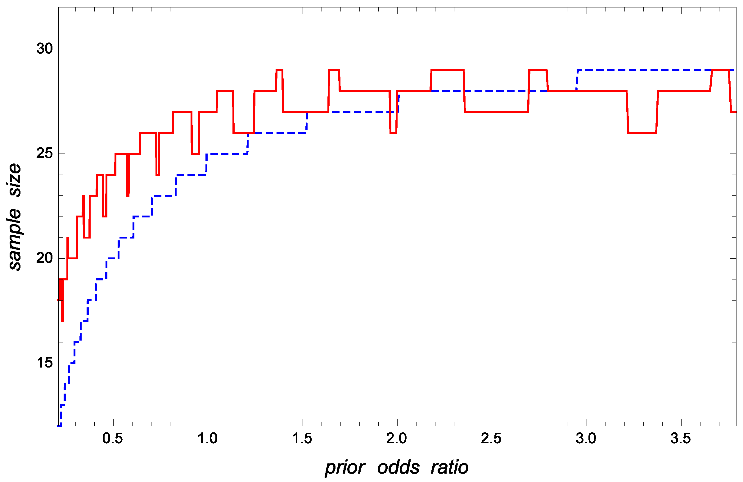
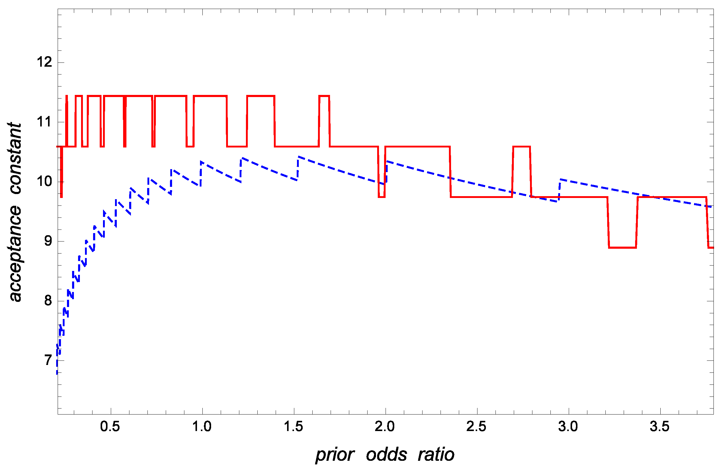
As graphical illustrations of the influence of r on the optimal and approximate sampling inspection schemes, Figure 1 and Figure 2 show the values of the approximate and optimal sample sizes and acceptance constants, respectively, versus r when ${\lambda }_0=0.3,$ ${\lambda }_1=0.7,$ $d_0=d_1=1,$ $\alpha =0.05$ and $\beta =0.10.$ Clearly, $n_a$ and $c_a$ are smaller than $n^{*}$ and $c^{*},$ respectively, when r is small. Otherwise, $(n_a,c_a)$ is a practical estimate of $(n^{*},c^{*}).$

An application to the production of paper is now discussed to exemplify the determination of optimal sampling plans based on prior odds ratio tests. The number of impurities discovered per inspection unit is typically the most important quality characteristic in paper manufacturing. In our case, a practitioner wishes to determine the best decision rule to reject or accept large lots of 0.49 m² sheets of paper, assuming that the number X of imperfections per sheet follows a $CMP(\lambda ,d)$ distribution with mean $\mu .$

The maximal Bayesian risks that the consumer and the producer are willing to incur in the development of a test plan for lot acceptance are $10\%$ and $5\%,$ respectively. Furthermore, the presence of sixty-five impurities is considered rejectable by the customer, whereas thirty-five blemishes per hundred sheets is deemed acceptable by the manufacturer. Thus, $\alpha =0.05,$ $\beta =0.10,$ and the acceptable and rejectable means are ${\mu }_0=0.35$ and ${\mu }_1=0.65.$ 

Table 3. Optimal and approximate plans, $(n^{*},c^{*})$ and $(n_a,c_a),$ and the corresponding Bayesian risks, BPR and BCR, when ${\mu }_0=0.35,$ ${\mu }_1=0.65,$ $\alpha =0.05,$ $\beta =0.10$ and $d_0=d_1=d$.

		Optimal Test Plan				Approximate Test Plan
d	${\mathit{p}}_0$	${\mathit{n}}^{*}$	${\mathit{c}}^{*}$	BPR	BCR	${\mathit{n}}_{\mathit{a}}$	${\mathit{c}}_{\mathit{a}}$	BPR	BCR
0.5	0.2	56	12.412	4.857%	9.455%	60	13.231	4.273%	8.455%
	0.5	55	14.524	4.749%	9.674%	53	13.881	5.114%	9.976%
	0.8	41	13.468	4.127%	9.864%	31	10.248	8.326%	10.567%
1.0	0.2	48	12.690	4.421%	9.735%	50	12.987	5.517%	6.300%
	0.5	47	14.547	4.985%	9.248%	45	13.894	5.361%	9.721%
	0.8	35	13.309	4.886%	9.349%	28	10.835	7.965%	10.22%
1.5	0.2	43	12.956	4.255%	9.445%	43	12.677	4.259%	9.528%
	0.5	43	15.057	4.844%	8.594%	40	14.040	4.365%	11.08%
	0.8	33	14.357	3.670%	9.623%	25	10.973	8.547%	9.896%

reports the optimal and approximate inspection schemes, $(n^{*},c^{*})$ and $(n_a,c_a),$ and their corresponding Bayesian risks when ${\mu }_0=0.35,$ ${\mu }_1=0.65,$ $d_0=d_1=d,$ $\alpha =0.05$ and $\beta =0.10$ for $d=0.5,$ $1.0,$ $1.5$ and $p_0=0.2,$ $0.5,$ $0.8.$

According to Table 3, if the acceptable and rejectable means, ${\mu }_0$ and ${\mu }_1,$ are fixed, the optimal sample size $n^{*}$ is reduced when the dispersion parameter d assumed by the manufacturer and customer increases. Therefore, the required sample size in the Poisson case is a lower bound of $n^{*}$ when the dispersion parameter is $d<1$ and an upper bound of $n^{*}$ when $d>1.$ For example, if $p_0=0.8,$ the minimal sample size $n^{*}=35$ when $d=1$ is a lower/upper bound of the value of $n^{*}$ when the dispersion parameter d is less/greater than $1.$ Clearly, the needed sample size increases when the observed random sample is over-dispersed compared to the Poisson distribution. For instance, if $p_0=0.5,$ the optimal sample size is $n^{*}=47$ when $d=1,$ whereas $n^{*}=55$ if $d=0.5.$

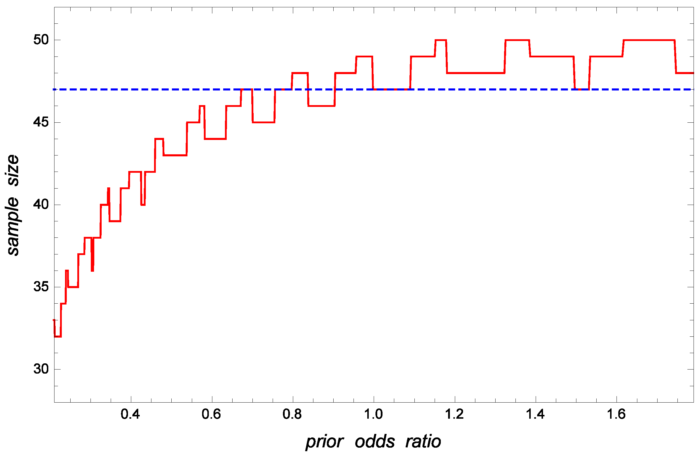
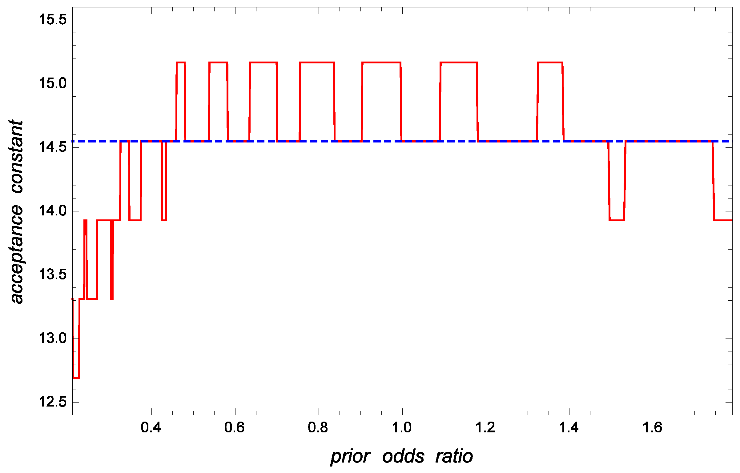
For illustrative and comparative purposes, Figure 3 displays the optimal sample size under the frequentist perspective $n_f=47$ and the optimal Bayesian sample size $n^{*}$ as a function of the prior odds ratio when ${\mu }_0=0.35,$${\mu }_1=0.65,$$d_0=d_1=1,$$\alpha =0.05$ and $\beta =0.10.$ The corresponding acceptance constants $c_f=14.5474$ and $c^{*}$ are shown in Figure 4. In view of these figures, it is evident that the Bayesian approach greatly decreases the required sample size and acceptance constant when the prior lot acceptability, $p_0=Pr\left(H_0\right)$, is high; i.e., when the prior odds ratio r is low. In the non-informative case, the best frequentist and Bayesian plans are quite similar.

7. Concluding Remarks

Lot acceptance sampling is widely used in industrial quality control to develop inspection schemes for defects per unit. The CMP model is a plausible generalization of the Poisson law that adds a parameter to represent the dispersion level. Assuming the presence of prior information on the production process, this paper has determined the best test plans for lot acceptance purposes when the number of minor defects per unit has a CMP distribution.

The proposed test plan for screening lots protects the consumer and the producer at the requested confidence levels and minimizes the sampling inspection effort. Mixed-integer nonlinear programming problems were solved through Monte Carlo simulation to determine the best inspection schemes based on posterior odds ratio tests. An explicit asymptotic approximation of the best plan was used as a starting point for iteratively searching the optimal scheme, which is of exceeding importance because the calculation of the optimal plan can be very computer intensive. The presented results were applied to the production of paper and glass.

The suggested approach is practically an extension of the classical frequentist perspective because both are quite similar in the non-informative case. Nonetheless, note that a classical statistician considers a probability is a frequency, whereas a Bayesian views a probability as a degree of belief. Our setting offers some advantages to the decision-maker. In particular, the producer and the consumer may assign different probabilities to the lot acceptability, even if they have identical background knowledge. A convenient way of combining new sample evidence with prior beliefs is also provided. Bayes’ rule can be used to continually update the posterior odds ratio as new subjective or objective information is acquired. In general, the inclusion of the dispersion parameter in the underlying probability distribution leads to improved decision rules for lot disposition based on under- or over-dispersed samples. Moreover, the incorporation of prior knowledge provides more precise assessments of the actual consumer and producer risks, as well as substantial savings in sample size when the prior lot acceptability is high.

References

- Baklizi, A.; El Masri, A.E.Q. Acceptance sampling based on truncated life tests in the Birnbaum Saunders model. Risk Anal. 2004, 24, 1453–1457. [Google Scholar] [CrossRef] [PubMed]
- Balamurali, S.; Jun, C.-H. Multiple dependent state sampling plans for lot acceptance based on measurement data. Eur. J. Oper. Res. 2007, 180, 1221–1230. [Google Scholar] [CrossRef]
- Tsai, T.-R.; Lu, Y.-T.; Wu, S.-J. Reliability sampling plans for Weibull distribution with limited capacity of test facility. Comput. Ind. Eng. 2008, 55, 721–728. [Google Scholar] [CrossRef]
- Lee, W.-C.; Wu, J.-W.; Hong, C.-W. Assessing the lifetime performance index of products with the exponential distribution under progressively type II right censored samples. J. Comput. Appl. Math. 2009, 231, 648–656. [Google Scholar] [CrossRef] [Green Version]
- Lu, W.; Tsai, T.-R. Interval censored sampling plans for the gamma lifetime model. Eur. J. Oper. Res. 2009, 192, 116–124. [Google Scholar] [CrossRef]
- Aslam, M.; Azam, M.; Jun, C.-H. A mixed repetitive sampling plan based on process capability index. Appl. Math. Model. 2013, 37, 10027–10035. [Google Scholar] [CrossRef]
- Fernández, A.J. Optimum attributes component test plans for k-out-of-n:F Weibull systems using prior information. Eur. J. Oper. Res. 2015, 240, 688–696. [Google Scholar] [CrossRef]
- Wu, C.-W.; Shu, M.-H.; Nugroho, A.A.; Kurniati, N. A flexible process-capability-qualified resubmission-allowed acceptance sampling scheme. Comput. Ind. Eng. 2015, 80, 62–71. [Google Scholar] [CrossRef]
- Wu, C.-W.; Lee, A.H.I.; Liu, S.-W.; Shih, M.-H. Capability-based quick switching sampling system for lot disposition. Appl. Math. Model. 2017, 52, 131–144. [Google Scholar] [CrossRef]
- Qin, R.; Cudney, E.A.; Hamzic, Z. An optimal plan of zero-defect single-sampling by attributes for incoming inspections in assembly lines. Eur. J. Oper. Res. 2015, 246, 907–915. [Google Scholar] [CrossRef]
- Lee, A.H.I.; Wu, C.-W.; Wang, Z.-H. The construction of a modified sampling scheme by variables inspection based on the one-sided capability index. Comput. Ind. Eng. 2018, 122, 87–94. [Google Scholar] [CrossRef]
- Roy, S. Bayesian accelerated life test plans for series systems with Weibull component lifetimes. Appl. Math. Model. 2018, 62, 383–403. [Google Scholar] [CrossRef]
- Algarni, A. Group Acceptance Sampling Plan Based on New Compounded Three-Parameter Weibull Model. Axioms 2022, 11, 438. [Google Scholar] [CrossRef]
- Alyami, S.A.; Elgarhy, M.; Elbatal, I.; Almetwally, E.M.; Alotaibi, N.; El-Saeed, A.R. Fréchet Binomial Distribution: Statistical Properties, Acceptance Sampling Plan, Statistical Inference and Applications to Lifetime Data. Axioms 2022, 11, 389. [Google Scholar] [CrossRef]
- Fernández, A.J. Optimal defects-per-unit acceptance sampling plans using truncated prior distributions. IEEE Trans. Reliab. 2014, 63, 634–645. [Google Scholar] [CrossRef]
- Anbazhagan, N.; Wang, J.; Gomathi, D. Base stock policy with retrial demands. Appl. Math. Model. 2013, 37, 4464–4473. [Google Scholar] [CrossRef]
- Alizadeh, M.; Eskandari, H.; Sajadifar, S.M. A modified (S-1,S) inventory system for deteriorating items with Poisson demand and non-zero lead time. Appl. Math. Model. 2014, 38, 699–711. [Google Scholar] [CrossRef]
- Chen, K.-S.; Yang, C.-M. Developing a performance index with a Poisson process and an exponential distribution for operations management and continuous improvement. J. Comput. Appl. Math. 2018, 343, 737–747. [Google Scholar] [CrossRef]
- Chuang, H.H.-C. Fixing shelf out-of-stock with signals in point-of-sale data. Eur. J. Oper. Res. 2018, 270, 862–872. [Google Scholar] [CrossRef]
- Wan, Q.; Liu, C.; Wu, Y.; Zhou, W. A TBE control chart-based maintenance policy for a service facility. Comput. Ind. Eng. 2018, 126, 136–148. [Google Scholar] [CrossRef]
- Fernández, A.J. Most powerful lot acceptance test plans from dispersed nonconformity counts. Int. J. Adv. Manuf. Technol. 2017, 90, 233–240. [Google Scholar] [CrossRef]
- Conway, R.W.; Maxwell, W.L. A queuing model with state dependent service rates. J. Ind. Eng. 1962, 12, 132–136. [Google Scholar]
- Shmueli, G.; Minka, T.; Kadane, J.B.; Borle, S.; Boatwright, P.B. A useful distribution for fitting discrete data: Revival of the Conway-Maxwell-Poisson distribution. Appl. Stat. 2005, 54, 127–142. [Google Scholar] [CrossRef]
- Sellers, K.F.; Borle, S.; Shmueli, G. The COM-Poisson model for count data: A survey of methods and applications. Appl. Stoch. Model. Bus. Ind. 2012, 28, 104–116. [Google Scholar] [CrossRef]
- Francis, R.A.; Geedipally, S.R.; Guikema, S.D.; Dhavala, S.S.; Lord, D.; LaRocca, S. Characterizing the performance of the Conway-Maxwell-Poisson generalized linear model. Risk Anal. 2012, 32, 167–183. [Google Scholar] [CrossRef] [Green Version]
- Zhu, F. Modeling time series of counts with COM-Poisson INGARCH models. Math. Comput. Model. 2012, 56, 191–203. [Google Scholar] [CrossRef]
- Santarelli, M.F.; Della Latta, D.; Scipioni, M.; Positano, V.; Landini, L. A Conway-Maxwell-Poisson (CMP) model to address data dispersion on positron emission tomography. Comput. Biol. Med. 2016, 77, 90–101. [Google Scholar] [CrossRef] [PubMed] [Green Version]
- Torney, D.C. Bayesian analysis of binary sequences. J. Comput. Appl. Math. 2005, 175, 231–243. [Google Scholar] [CrossRef] [Green Version]
- Fernández, A.J. Bayesian estimation based on trimmed samples from Pareto populations. Comput. Stat. Data Anal. 2006, 51, 1119–1130. [Google Scholar] [CrossRef]
- Fernández, A.J. Weibull inference using trimmed samples and prior information. Stat. Pap. 2009, 50, 119–136. [Google Scholar] [CrossRef]
- Fernández, A.J. Computing tolerance limits for the lifetime of a k-out-of-n:F system based on prior information and censored data. Appl. Math. Model. 2014, 38, 548–561. [Google Scholar] [CrossRef]
- Yan, L.; Yang, F.; Fu, C. A Bayesian inference approach to identify a Robin coefficient in one-dimensional parabolic problems. J. Comput. Appl. Math. 2009, 231, 840–850. [Google Scholar] [CrossRef] [Green Version]
- Lee, W.-C.; Wu, J.-W.; Hong, M.-L.; Lin, L.-S.; Chan, R.-L. Assessing the lifetime performance index of Rayleigh products based on the Bayesian estimation under progressive type II right censored samples. J. Comput. Appl. Math. 2011, 235, 1676–1688. [Google Scholar] [CrossRef]
- Jaheen, Z.F.; Okasha, H.M. E-Bayesian estimation for the Burr type XII model based on type-2 censoring. Appl. Math. Model. 2011, 35, 4730–4737. [Google Scholar] [CrossRef]
- Asl, M.N.; Belaghi, R.A.; Bevrani, H. Classical and Bayesian inferential approaches using Lomax model under progressively type-I hybrid censoring. J. Comput. Appl. Math. 2018, 343, 397–412. [Google Scholar] [CrossRef]
- He, D.; Wang, Y.; Chang, G. Objective Bayesian analysis for the accelerated degradation model based on the inverse Gaussian process. Appl. Math. Model. 2018, 61, 341–350. [Google Scholar] [CrossRef]
- Alotaibi, R.; Nassar, M.; Ghosh, I.; Rezk, H.; Elshahhat, A. Inferences of a Mixture Bivariate Alpha Power Exponential Model with Engineering Application. Axioms 2022, 11, 459. [Google Scholar] [CrossRef]
- Yousef, M.M.; Hassan, A.S.; Alshanbari, H.M.; El-Bagoury, A.-A.H.; Almetwally, E.M. Bayesian and Non-Bayesian Analysis of Exponentiated Exponential Stress–Strength Model Based on Generalized Progressive Hybrid Censoring Process. Axioms 2022, 11, 455. [Google Scholar] [CrossRef]
- Fernández, A.J. Optimal schemes for resubmitted lot acceptance using previous defect count data. Comput. Ind. Eng. 2015, 87, 66–73. [Google Scholar] [CrossRef]
Figure 1.
Optimal (solid line) and approximate (dashed line) sample sizes, and versus the prior odds ratio when and
Figure 2.
Optimal (solid line) and approximate (dashed line) acceptance constants, and versus the prior odds ratio when and
Figure 3.
Optimal Bayesian (solid line) and frequentist (dashed line) sample sizes, and versus the prior odds ratio when and
Figure 4.
Optimal Bayesian (solid line) and frequentist (dashed line) acceptance constants, and versus the prior odds ratio when and