Simulation of Marine Debris Path Using Mathematical Model in the Gulf of Thailand

Abstract

Marine debris is an important environmental problem that affects aquatic animals, ecosystems, economy, society, and humans. This research aims to simulate the path of marine debris in the Gulf of Thailand using a mathematical model that includes two models: the Oceanic Model (OCM), which is based on the Shallow Water Equations (SWE), and the Lagrangian Particle Tracking (LPT) model. The OCM is the partial derivative equation system solved by the finite difference method to satisfy the Arakawa C-grid and the splitting method. The LPT model includes the current velocity, wind velocity at 10 m above sea level, random walk term, and the buoyancy ratio of marine debris with six cases, which are 100:1, 10:1, 1:1, 0:1, 1:10, and 1:100. The current velocity from OCM is applied to the LPT model. This research uses a garbage boat that capsized near Koh Samui on 1 August 2020 as a case study. The simulated current velocity of OCM is compared with Ocean Surface Current Analyses Real-time (OSCAR) data. The Root Mean Square Error (RMSE) of u-velocity is 0.070 m/s, and that of v-velocity is 0.058 m/s. The simulation of the marine debris’s path from the LPT model demonstrates the movement to Koh Samui, Koh Taen, Koh Wang Nai, Koh Wang Nok, Koh Rap, the east coast of Nakorn Si Thammarat province, Phu Quoc Island of Vietnam and the middle of the Gulf of Thailand with the different buoyancy ratios and time durations.

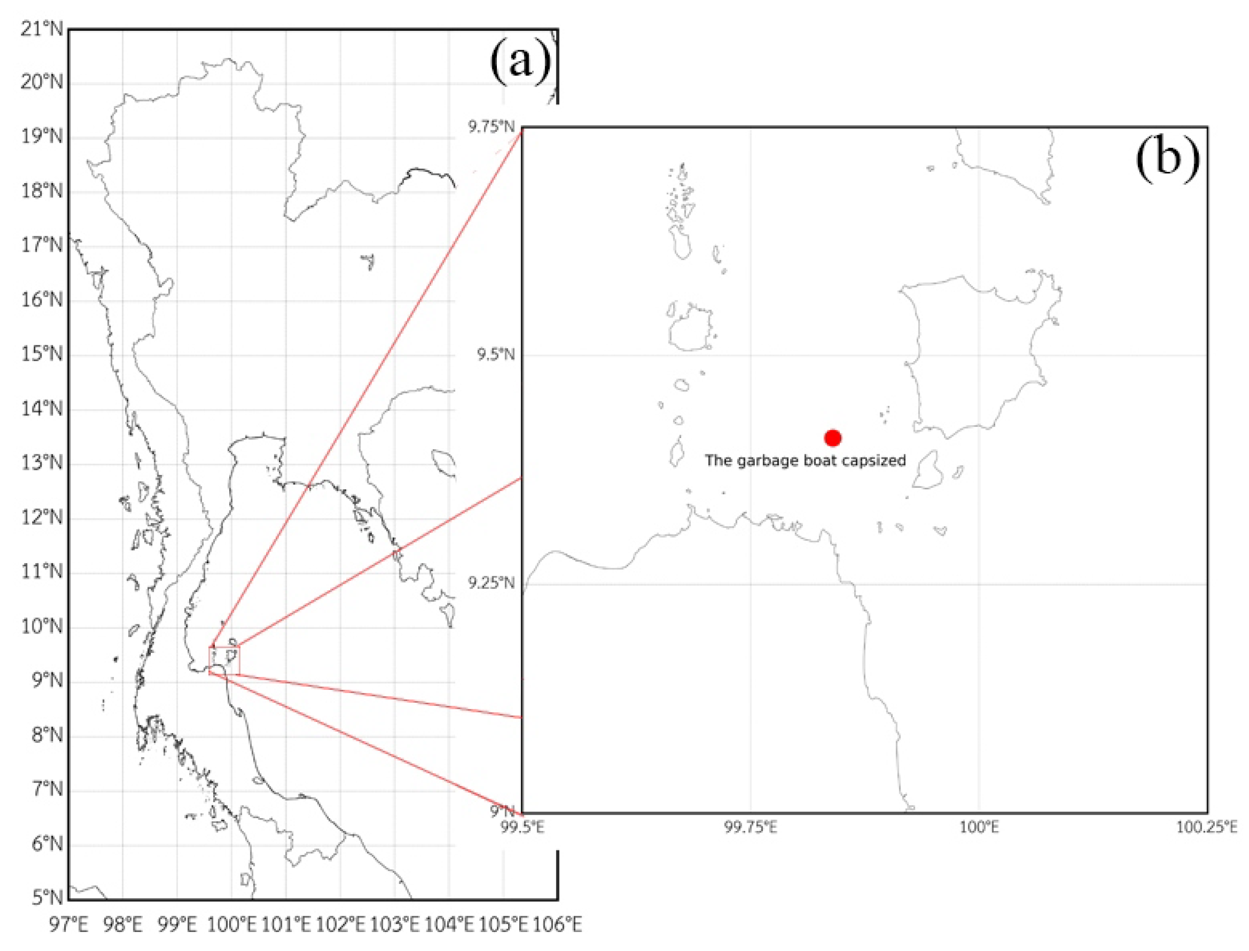
1. Introduction

Marine debris is the most important environmental pollution such as marine debris generated by the mismanagement of waste. Marine debris also affects aquatic animals, causing injury or death that affects the ecosystem. Finally, humans and the economy are affected. For example, through aquatic animals, humans will ingest microplastics, and increased marine debris affects tourism. The Thailand Development Research Institute (TDRI) reports that Thailand has the 10th largest amount of marine debris (2020). It is classified as the amount of plastic waste that is not properly managed, a total of 1.03 million tons/year. Plastic waste leaks into the sea at a rate of about 0.41 million tons/year. Most of the waste is plastic, accounting for 12%, while foam boxes account for 10%, food packaging 8%, plastic bags 8%, glass bottles 7%, plastic bottles 7%, and straws 5% [1] After macroplastics travel to the sea, they will decompose into microplastics and move with the current from the source of microplastics to the nearshore region [2]. Abolfathi and Pearson [3,4] study the particle hydrodynamics and consider the dispersion and diffusion of micro-substances or solute dispersion using waves and currents in the nearshore area.

The Gulf of Thailand (GoT) is the shallow inlet of the South China Sea (SCS) and is located from 6 to 13.5${}^{\circ }\mathrm{N}$ latitude and 99 to 105${}^{\circ }\mathrm{E}$ longitude (Figure 1a). It is a semi-enclosed bay by the coast of the Malay Peninsula in the west and the ground of Southeast Asia in the north and east. The southeastern part of the GoT is an opening between the Laem Yuan in Vietnam and Malaysia’s Kota Bharu that connects with the SCS. The average depth is about 44 m, and the deepest part of the bay is about 86 m deep.

The Oceanic Model (OCM) is the model for studying oceanic variables such as current velocity and sea surface elevation. It has been applied to study in many ways, i.e., using the OCM to detect the storm surge or study current velocity and sea surface elevation from the tsunami. Ren et al. [5,6] study the shallow water equations (SWE) to consider wave amplitude and currents in the SCS with tsunami events that occur from earthquakes in the Manila subduction zone by using the OCM based on the SWE and the second-order Godunov method to discretize the SWE. The region with a high hazard risk is considered, and tsunami information is applied to develop a tsunami warning in 5 min.

In this paper, we simulate the path of marine debris in the GoT from a starting point (Figure 1b) using two models: the OCM and the Lagrangian Particle Tracking (LPT) model. The surface current velocity of the OCM is compared with the surface current of the Ocean Surface Current Analyses Real-time (OSCAR) model and then the LPT model used the surface current velocity as initial data.

2. Mathematical Method

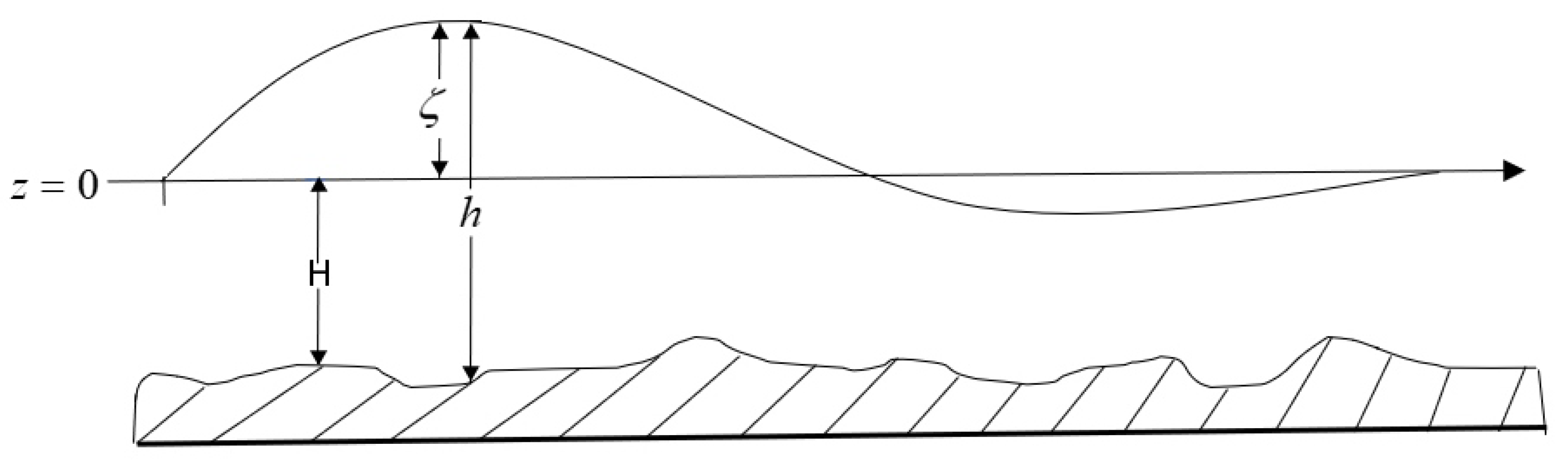
2.1. The Oceanic Model

The Oceanic Model (OCM) is based on two-dimensional shallow water equations (SWE) for computing current velocity and sea surface elevation (Figure 2). The SWE include the continuity equation and momentum equations on the x and y-axis as Equations (1)–(3).

$$\begin{array}{cc}\hfill \frac{\partial \zeta }{\partial t}+\frac{\partial \left(hu\right)}{\partial x}+\frac{\partial \left(hv\right)}{\partial y}& =0,\hfill \end{array}$$

(1)

$$\begin{array}{cc}\hfill \frac{\partial u}{\partial t}+u\frac{\partial u}{\partial x}+v\frac{\partial u}{\partial y}-fv& =-g\frac{\partial \zeta }{\partial x}-\frac{1}{\rho }\frac{\partial p_a}{\partial x}+F_{sx}-F_{bx},\hfill \end{array}$$

(2)

$$\begin{array}{cc}\hfill \frac{\partial v}{\partial t}+u\frac{\partial v}{\partial x}+v\frac{\partial v}{\partial y}+fu& =-g\frac{\partial \zeta }{\partial y}-\frac{1}{\rho }\frac{\partial p_a}{\partial y}+F_{sy}-F_{by},\hfill \end{array}$$

(3)

let

$$\begin{array}{cc}\hfill & F_{sx}=\frac{{\tau }_{sx}}{\rho h}=\frac{{\rho }_a{C}_D\left|W\right|W_x}{\rho h},F_{sy}=\frac{{\tau }_{sy}}{\rho h}=\frac{{\rho }_a{C}_D\left|W\right|W_y}{\rho h},\hfill \\ & F_{bx}=\frac{{\tau }_{bx}}{\rho h}=\frac{\rho r_b\left|V\right|u}{\rho h},F_{by}=\frac{{\tau }_{by}}{\rho h}=\frac{\rho r_b\left|V\right|v}{\rho h},\hfill \end{array}$$

where $u,v$ are the current velocity on the x and y-axis, respectively, $\zeta$ is the sea surface elevation, h is the total water depth (the sum of sea surface elevation and bottom topography (H)), $p_a$ is air pressure, f is the Coriolis force, $\rho$ is the density of water, ${\rho }_a$ is the density of air, g is the gravity constant, $W_x,W_y$ are the wind velocity on the x and y-axis, $r_b$ is the coefficient of the bottom friction, $C_D$ is the coefficient of the wind stress, $\left|W\right|$ is the wind speed, $\left|V\right|$ is the current speed, ${\tau }_{sx},{\tau }_{sy}$ are the surface stress by the wind velocity on the x and y-axis, ${\tau }_{bx},{\tau }_{by}$ are the bottom stress by the current velocity, $F_{sx},F_{sy}$ are the friction force on the surface, $F_{bx},F_{by}$ are the friction force on the bottom.

From Guo et al. [7], the defined transformation variables are given by

$$\begin{array}{cc}\hfill \mathsf{\Phi }& =\sqrt{gh}=\sqrt{g\left(H+\zeta \right)}=\sqrt{gH+g\zeta }=\sqrt{gH+\phi },\hfill \\ \hfill U& =\sqrt{gh}u=\mathsf{\Phi }u,\hfill \\ \hfill V& =\sqrt{gh}v=\mathsf{\Phi }v.\hfill \end{array}$$

Multiplying Equation (1) by g and Equations (2) and (3) by $\mathsf{\Phi }$, we obtain the transformation of the SWE as shown in Equations (4)–(6):

$$\begin{array}{cc}\hfill \frac{\partial \phi }{\partial t}+\frac{\partial \left(\mathsf{\Phi }U\right)}{\partial x}+\frac{\partial \left(\mathsf{\Phi }V\right)}{\partial y}& =0,\hfill \end{array}$$

(4)

$$\begin{array}{cc}\hfill \frac{\partial U}{\partial t}+\frac{1}{2}\left(u\frac{\partial U}{\partial x}+\frac{\partial uU}{\partial x}\right)+\frac{1}{2}\left(v\frac{\partial U}{\partial y}+\frac{\partial vU}{\partial y}\right)-fV& =-\mathsf{\Phi }\frac{\partial \phi }{\partial x}-\frac{\mathsf{\Phi }}{\rho }\frac{\partial p_a}{\partial x}+\mathsf{\Phi }{F}_{sx}-kU,\hfill \end{array}$$

(5)

$$\begin{array}{cc}\hfill \frac{\partial V}{\partial t}+\frac{1}{2}\left(u\frac{\partial V}{\partial x}+\frac{\partial \left(uV\right)}{\partial x}\right)+\frac{1}{2}\left(v\frac{\partial V}{\partial y}+\frac{\partial vV}{\partial y}\right)+fU& =-\mathsf{\Phi }\frac{\partial \phi }{\partial y}-\frac{\mathsf{\Phi }}{\rho }\frac{\partial p_a}{\partial y}+\mathsf{\Phi }{F}_{sy}-kV.\hfill \end{array}$$

(6)

Let

$$\begin{array}{cc}\hfill \mathsf{\Phi }{F}_{sx}& =\frac{{\rho }_a{C}_{D}g{\left(W_x^2+W_y^2\right)}^{1/2}{W}_x}{\rho \mathsf{\Phi }},\mathsf{\Phi }{F}_{sy}=\frac{{\rho }_a{C}_{D}g{\left(W_x^2+W_y^2\right)}^{1/2}{W}_y}{\rho \mathsf{\Phi }},\hfill \\ \hfill kU& =\frac{r_b{\left(U^2+V^2\right)}^{1/2}U}{{\mathsf{\Phi }}^3}=\mathsf{\Phi }{F}_{bx},kV=\frac{r_b{\left(U^2+V^2\right)}^{1/2}V}{{\mathsf{\Phi }}^3}=\mathsf{\Phi }{F}_{by}.\hfill \end{array}$$

Equations (4)–(6) can be written in the vector form as follows:

$$\begin{array}{cc}\hfill \frac{\partial \phi }{\partial t}+\nabla ·\left(\mathsf{\Phi }\mathrm{V}\right)& =0,\hfill \end{array}$$

(7)

$$\begin{array}{cc}\hfill \frac{\partial \mathbf{V}}{\partial t}+\left(\mathbf{v}·\nabla \right)\mathbf{V}+\frac{1}{2}\left(\nabla ·\mathbf{v}\right)+f\left(\mathbf{k}\times \mathbf{V}\right)& =-\mathsf{\Phi }\nabla \phi -\frac{\mathsf{\Phi }}{\rho }\nabla p_a+\mathsf{\Phi }{\mathbf{F}}_s-k\mathbf{V},\hfill \end{array}$$

(8)

where $\mathbf{V}=\left(U,V\right),\mathbf{v}=\left(u,v\right)$ and ${\mathbf{F}}_{\mathrm{s}}=\left(F_{sx},F_{sy}\right).$ We define the domain S and boundary C of S in the OCM; the initial condition is set at $t=0$, and the boundary conditions are set as shown below. Initial condition:

$$\begin{array}{c}\hfill U\left(x,y,0\right)=V\left(x,y,0\right)=\zeta \left(x,y,0\right)=0,\end{array}$$

Boundary condition:

$$\begin{array}{c}\hfill \mathbf{V}·\mathbf{n}=0,\end{array}$$

where $\mathbf{n}$ is the unit outward normal to C.

Applying the initial, boundary condition and integrating on the domain S to Equations (7) and (8), the following equation of mass conservation and energy conservation are obtained

$$\begin{array}{c}\hfill \frac{\partial }{\partial t}\underset{s}{\int \int }\phi dS=0,\end{array}$$

and

$$\frac{\partial }{\partial t}\underset{S}{\int \int }\left[\frac{1}{2}\left({\left|\mathbf{V}\right|}^2+{\phi }^2\right)\right]dS=\frac{\partial }{\partial t}\underset{S}{\int \int }\left[\frac{1}{2}\left(U^2+V^2+{\phi }^2\right)\right]dS=0.$$

2.2. Solving Method

The SWE are solved by the finite difference method and the splitting method [7] with the Arakawa C-grid [8].

2.2.1. The Finite Difference Method (FDM)

The derivative terms in the SWE can be replaced by finite difference. We use forward-finite difference approximation for the time derivative term and space derivative term as follows

$$\begin{array}{c}\hfill {\left(\frac{\partial f}{\partial t}\right)}_{i,j}^n\approx \frac{f_{i,j}^{n+1}-f_{i,j}^n}{\mathsf{\Delta }t},{\left(\frac{\partial f}{\partial x}\right)}_{i,j}^n\approx \frac{f_{i+1,j}^n-f_{i,j}^n}{\mathsf{\Delta }x},\mathrm{and}{\left(\frac{\partial f}{\partial y}\right)}_{i,j}^n\approx \frac{f_{i,j+1}^n-f_{i,j}^n}{\mathsf{\Delta }y},\end{array}$$

where f is an unknown function, $\mathsf{\Delta }t$ is the time interval, and $\mathsf{\Delta }x,\mathsf{\Delta }y$ are the distance intervals on the x and y-axis, respectively.

2.2.2. The Splitting Method

According to Guo et al. [7], the SWE contain three feature terms: a linear term, a nonlinear term, and a physical term. Assume $F\equiv U,V,$ or $\phi$, and we consider the splitting method as follows

$$\begin{array}{cc}\hfill \frac{\partial F}{\partial t}+AF& =0,\hfill \\ \hfill \frac{\partial F}{\partial t}+A_{1}F+A_{2}F+A_{3}F& =0.\hfill \end{array}$$

(9)

where $A_{1}F$ is the linear term, $A_{2}F$ is the nonlinear term, and $A_{3}F$ is the physical term. The algorithm of the splitting method is as follows

$$\begin{array}{c}\hfill \frac{F^{n+\frac{1}{3}}-F^n}{\mathsf{\Delta }t}+A_1\left[\frac{F^{n+\frac{1}{3}}-F^n}{2}\right]=0,\\ \hfill \frac{F^{n+\frac{2}{3}}-F^{n+\frac{1}{3}}}{\mathsf{\Delta }t}+A_2\left[\frac{F^{n+\frac{2}{3}}-F^{n+\frac{1}{3}}}{2}\right]=0,\\ \hfill \frac{F^{n+1}-F^{n+\frac{2}{3}}}{\mathsf{\Delta }t}+A_3\left[\frac{F^{n+1}-F^{n+\frac{2}{3}}}{2}\right]=0,\end{array}$$

and applying the algorithm of the splitting method in Equations (4)–(6) with the Arakawa C-grid, we rearrange the sets of equation into three parts. The first part is called the adjustment process for the linear term as follows:

$$\begin{array}{cc}\hfill U_{{}_{i+\frac{1}{2},j}}^{n+\frac{1}{3}}& =U_{{}_{i+\frac{1}{2},j}}^n+\mathsf{\Delta }{t}_1{\left[fV-\mathsf{\Phi }\frac{\partial \phi }{\partial x}\right]}_{i+\frac{1}{2},j}^{n+\frac{1}{3}},\hfill \\ \hfill V_{{}_{i+\frac{1}{2},j}}^{n+\frac{1}{3}}& =V_{{}_{i+\frac{1}{2},j}}^n-\mathsf{\Delta }{t}_1{\left[fU-\mathsf{\Phi }\frac{\partial \phi }{\partial y}\right]}_{i,j+\frac{1}{2}}^{n+\frac{1}{3}},\hfill \\ \hfill {\phi }_{i,j}^{n+\frac{1}{3}}& ={\phi }_{i,j}^n-\mathsf{\Delta }{t}_1{\left[\frac{\partial \left(\mathsf{\Phi }U\right)}{\partial x}+\frac{\partial \left(\mathsf{\Phi }V\right)}{\partial y}\right]}_{i,j}^{n+\frac{1}{3}},\hfill \end{array}$$

The second part is called the development process for the nonlinear term as follows:

$$\begin{array}{cc}\hfill U_{i+\frac{1}{2},j}^{n+\frac{2}{3}}& =U_{i+\frac{1}{2},j}^{n+\frac{1}{3}}-\mathsf{\Delta }{t}_2{\left[\frac{1}{2}\left[u\frac{\partial U}{\partial x}+\frac{\partial uU}{\partial x}\right]+\frac{1}{2}\left[v\frac{\partial U}{\partial y}+\frac{\partial vU}{\partial y}\right]\right]}_{{}^{i+\frac{1}{2},j}}^{n+\frac{2}{3}},\hfill \\ \hfill V_{i,j+\frac{1}{2}}^{n+\frac{2}{3}}& =V_{i,j+\frac{1}{2}}^{n+\frac{1}{3}}-\mathsf{\Delta }{t}_2{\left[\frac{1}{2}\left[u\frac{\partial V}{\partial x}+\frac{\partial \left(uV\right)}{\partial x}\right]+\frac{1}{2}\left[v\frac{\partial V}{\partial y}+\frac{\partial vV}{\partial y}\right]\right]}_{i,j+\frac{1}{2}}^{n+\frac{2}{3}},\hfill \\ \hfill {\phi }_{i,j}^{n+\frac{2}{3}}& ={\phi }_{i,j}^{n+\frac{1}{3}},\hfill \end{array}$$

The third part is called the dissipation process for the physical term as follows:

$$\begin{array}{cc}\hfill U_{i+\frac{1}{2},j}^{n+1}& =U_{i+\frac{1}{2},j}^{n+\frac{2}{3}}+\mathsf{\Delta }{t}_3{\left[-\frac{\mathsf{\Phi }}{\rho }\frac{\partial p_a}{\partial x}+\mathsf{\Phi }{F}_{sx}-kU\right]}_{i+\frac{1}{2},j}^{n+1},\hfill \\ \hfill V_{i,j+\frac{1}{2}}^{n+1}& =V_{i,j+\frac{1}{2}}^{n+\frac{2}{3}}+\mathsf{\Delta }{t}_3{\left[-\frac{\mathsf{\Phi }}{\rho }\frac{\partial p_a}{\partial y}+\mathsf{\Phi }{F}_{sy}-kV\right]}_{i,j+\frac{1}{2}}^{n+1},\hfill \\ \hfill {\phi }_{i,j}^{n+1}& ={\phi }_{i,j}^{n+\frac{2}{3}},\hfill \end{array}$$

where $\mathsf{\Delta }{t}_3=\mathsf{\Delta }{t}_2=M\mathsf{\Delta }{t}_1,$ and the value of M is between 5 and 10.

The data used in the OCM are the wind velocity at 10 m above sea level and surface pressure, which are the hourly reanalysis products derived from the Climate Data Store (CDS), with a horizontal resolution of 0.25 × 0.25 degrees. The topography dataset was obtained from the General Bathymetry Chart of the Ocean (GEBCO).

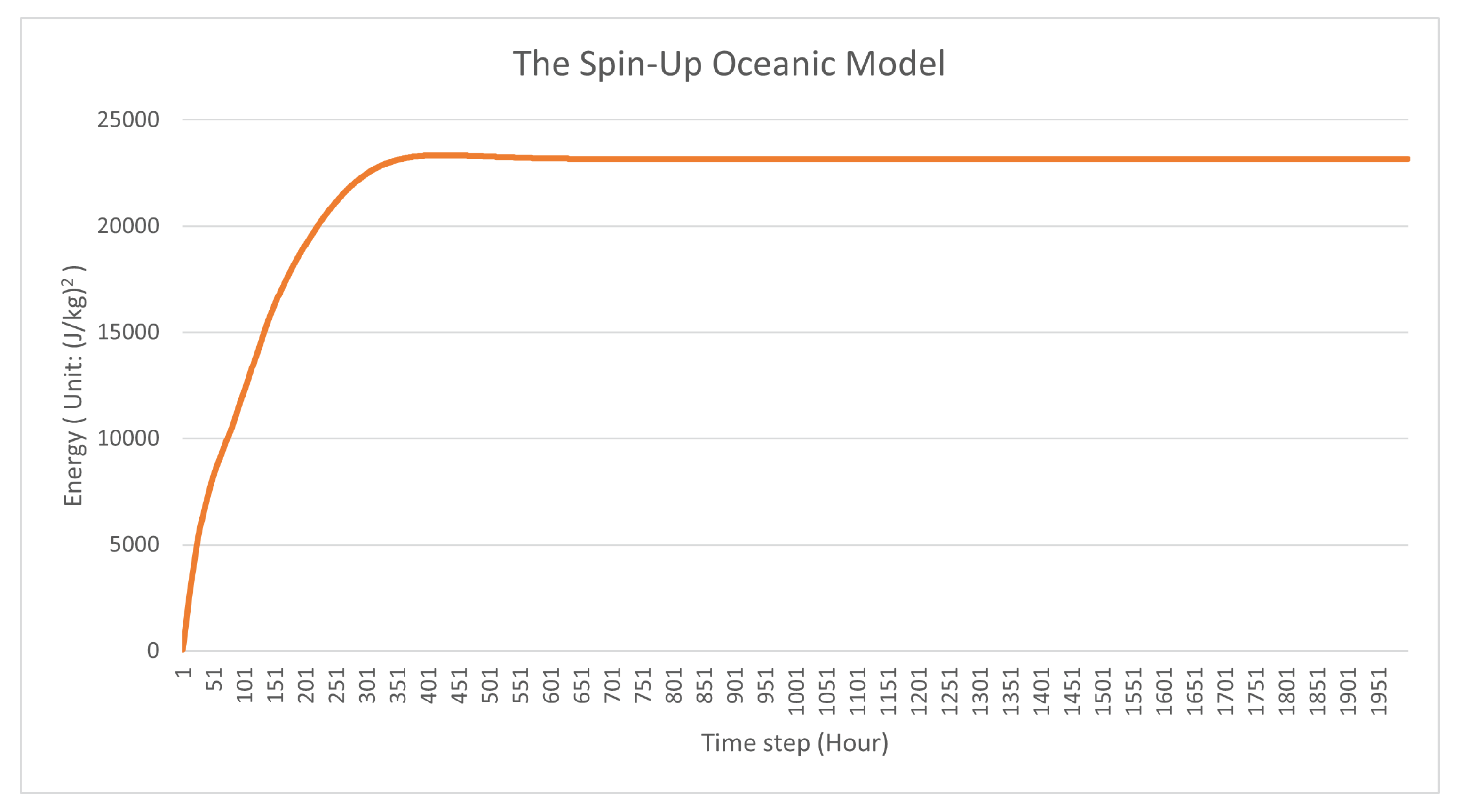
2.2.3. Spin-Up Method

The initial data for simulation of the OCM can be prepared by using the spin-up process, starting with the meteorological data at t = 0 to obtain U, V, and $\phi$ in the Equations (4)–(6) by using the splitting method for each time step with the grid size of 0.25 × 0.25 degrees and repeat until the total energy of OCM reaches an equilibrium state [9]. We define the total energy in discrete form as

$$\begin{array}{c}\hfill E^n=\sum _{j=0}^{ndy}\sum _{i=0}^{ndx}\frac{1}{2}\left({\left(U_{i,j}^n\right)}^2+{\left(V_{i,j}^n\right)}^2+{\left({\phi }_{i,j}^n\right)}^2\right),\end{array}$$

(10)

where n is the time step number, $ndx,ndy$ are the number of points in longitude and latitude, respectively, and the condition for the spin-up process is defined as

$$\begin{array}{c}\hfill \left|E^n-E^{n-1}\right|<{10}^{-3}.\end{array}$$

2.2.4. Root Mean Square Error

Root Mean Square Error (RMSE) is used to measure the differences between prediction and observation. In this case, the RMSE is calculated between the surface current velocity of the OCM and the OSCAR. The formulation of RMSE is as follows

$$\begin{array}{c}\hfill RMSE=\sqrt{\frac{{\displaystyle \sum _{i=1}^n}{\left(q_i-q_{oscar}\right)}^2}{n}},\end{array}$$

where q is the surface current velocity from the OCM, $q_{oscar}$ is the surface current velocity from the OSCAR, and n is the number of data.

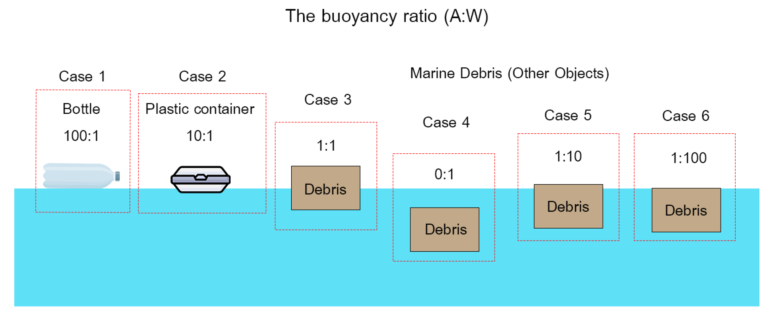
2.3. Lagrangian Particle Tracking Model

Based on the Lagrangian Particle Tracking (LPT) model by Carlson et al. [10], Seo et al. [11,12], and Yoon et al. [13], the authors develop the LPT model by considering controllable and uncontrollable factors. The controllable factors are the current and wind velocity, and the uncontrollable factor is the random walk term. The development of the LPT model is shown in Equation (10),

$$\begin{array}{c}\hfill {\overrightarrow{x}}_{i+1}\left(t+\mathsf{\Delta }t\right)={\overrightarrow{x}}_i\left(t\right)+\mathsf{\Delta }t·\overrightarrow{u}\left({\overrightarrow{x}}_i,t\right)+\left(k\sqrt{\frac{A}{W}}\mathsf{\Delta }t\right)·{\overrightarrow{w}}_{10m}\left({\overrightarrow{x}}_i,t\right)+\sqrt{2K_h\mathsf{\Delta }t}·\overrightarrow{R},\end{array}$$

(11)

where $\overrightarrow{x}=\left(x,y\right)$ is the position of marine debris, $\overrightarrow{u}=\left(u,v\right)$ is the current velocity along the x and y-axis, respectively, ${\overrightarrow{w}}_{10m}=\left(w_x,w_y\right)$ is the wind velocity at 10 m along the x and y-axis, respectively, $\overrightarrow{R}=\left(R_x,R_y\right)$ is the random number between −1 and 1 along the x and y-axis, k is the coefficient of wind pressure, $K_h$ is the horizontal diffusion (here, $K_h=2.09{\mathrm{m}}^2/\mathrm{s}$ for the GoT [14], $\mathsf{\Delta }t$ is the interval time, and W, A are the cross-section of floating marine debris to the wind direction below and above the sea surface, respectively.

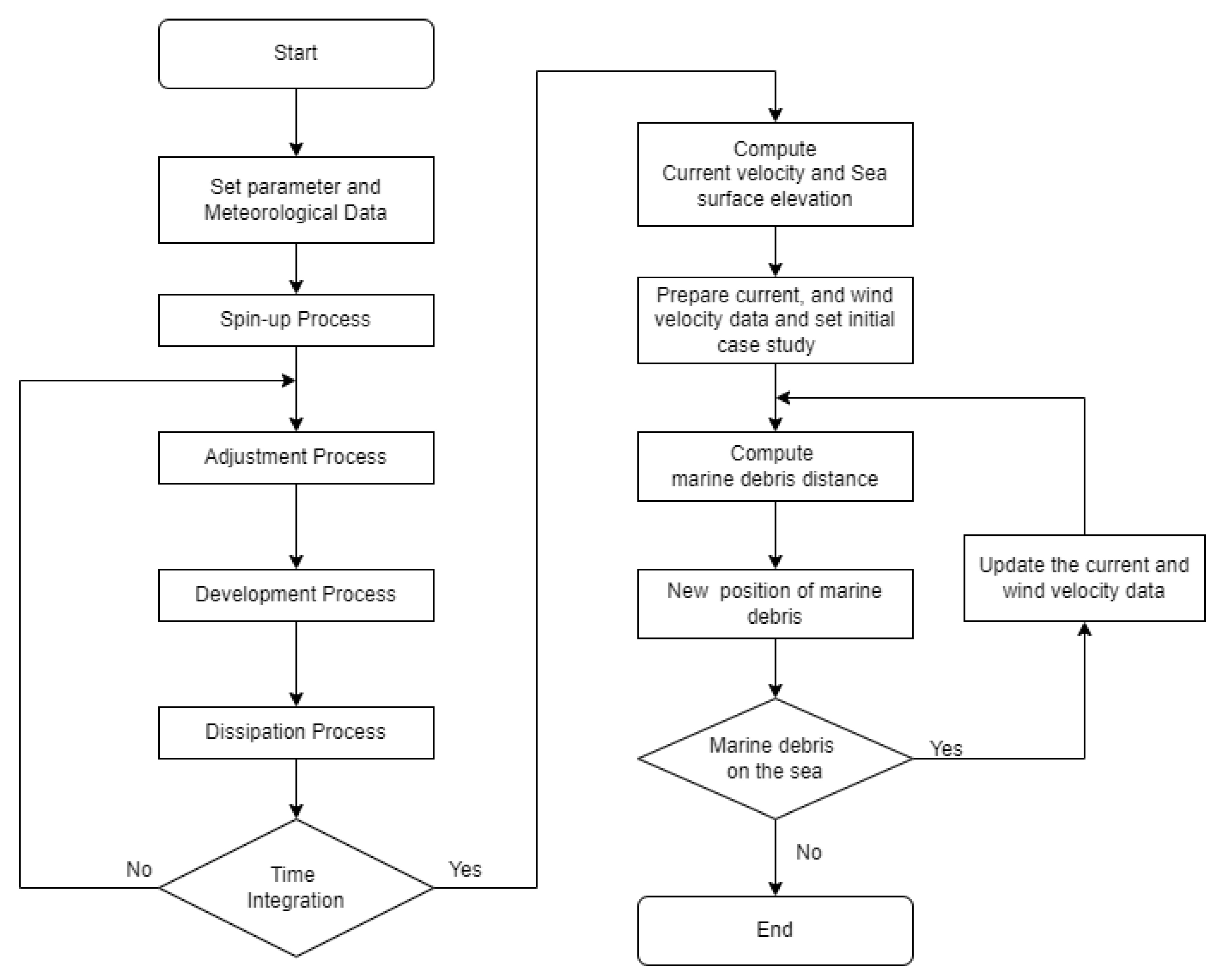
2.4. Operational Diagram

Figure 3 shows an operational diagram of the OCM and LPT model for the path and position of marine debris with the buoyancy ratio (Figure 4). Both the OCM and LPT model are written in Python language.

3. Results

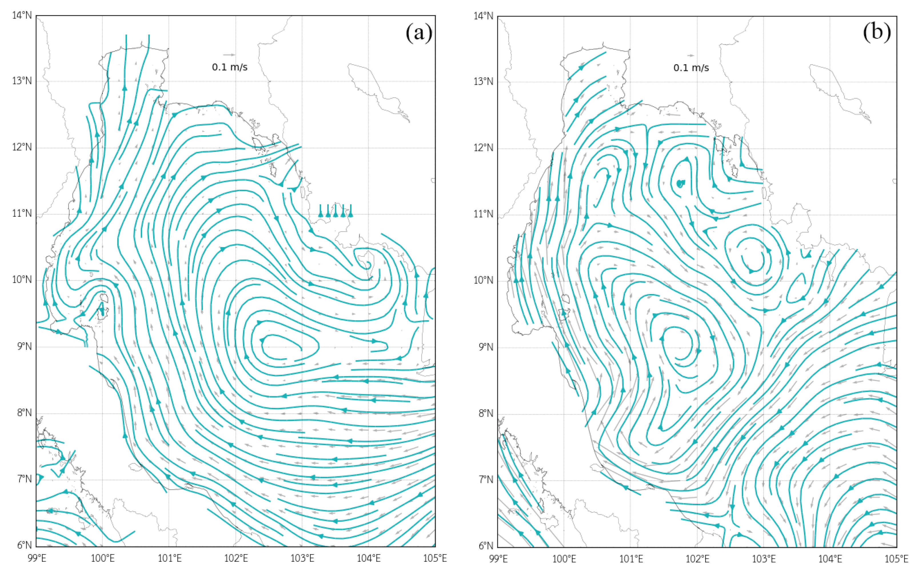
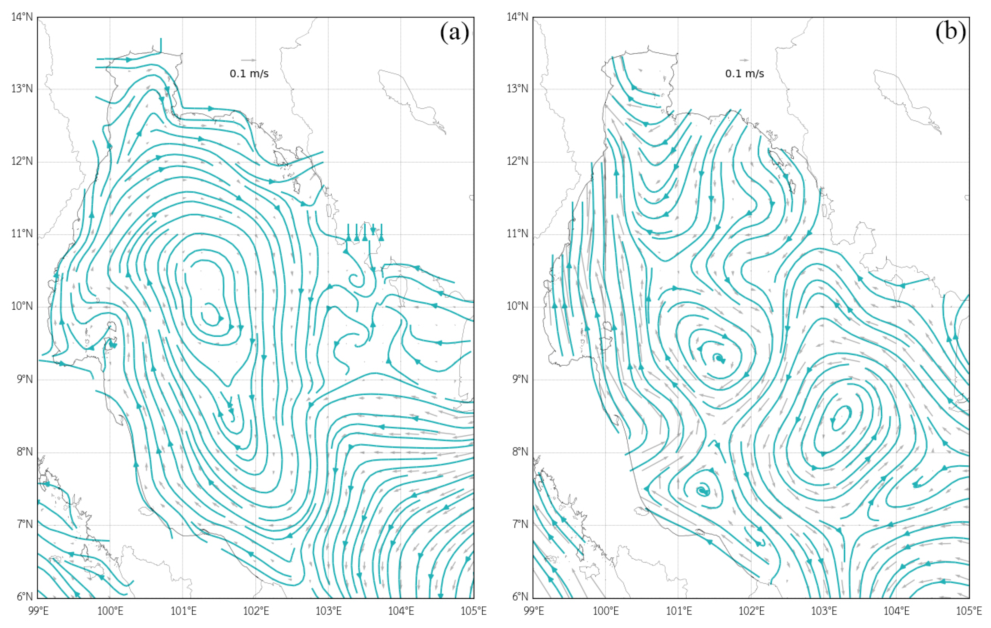
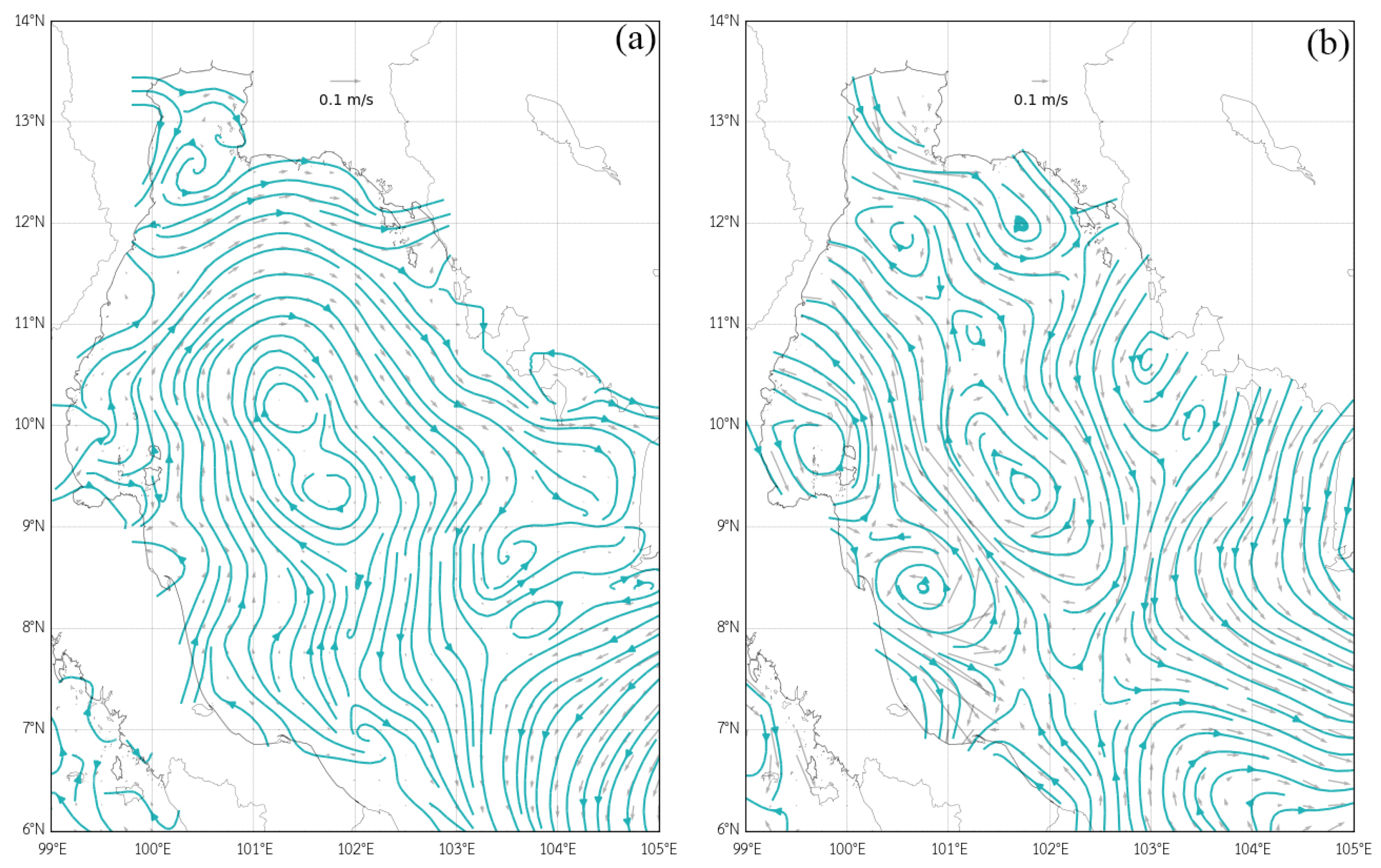
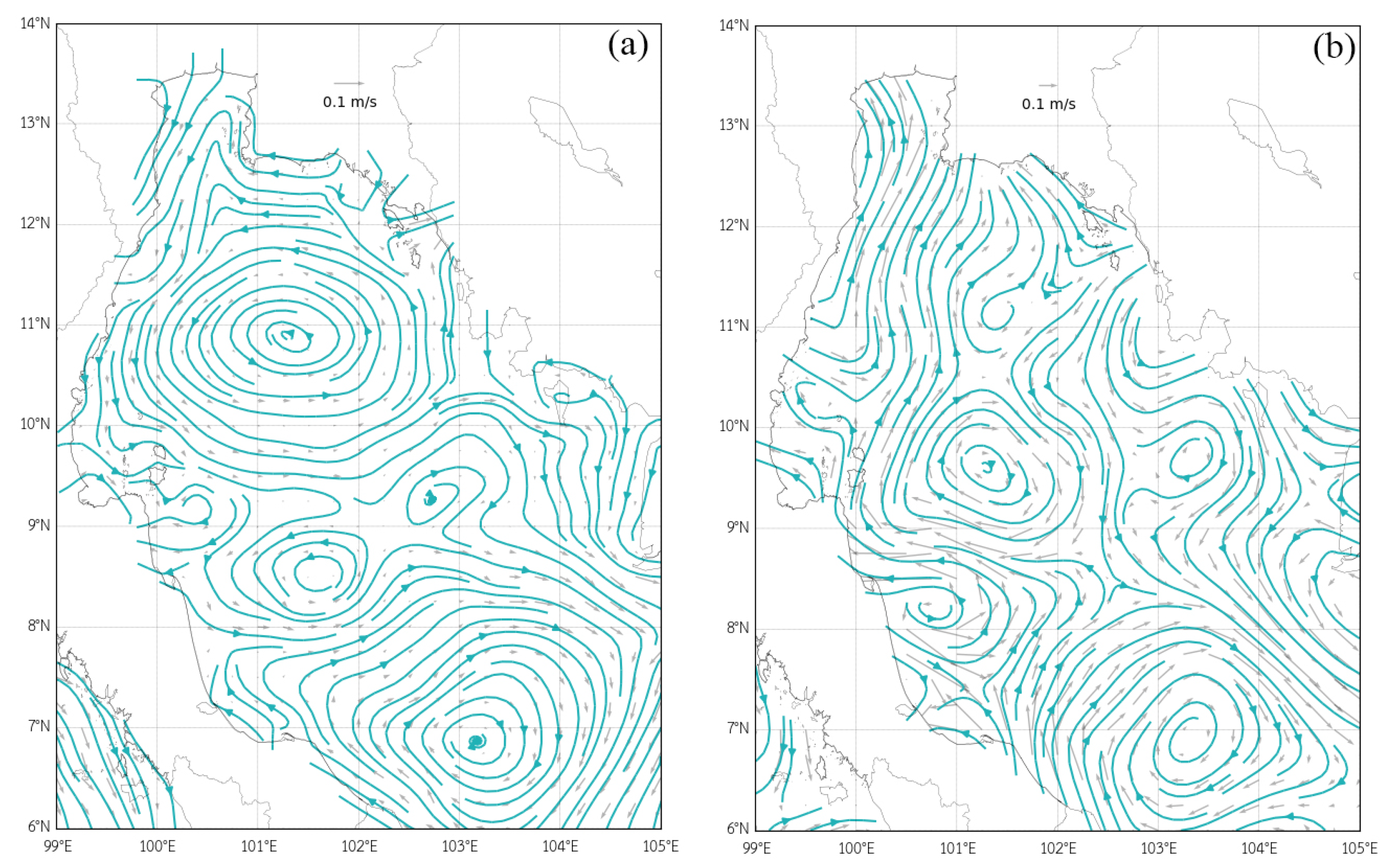
3.1. Oceanic Model

The resolution of OCM is 0.25 × 0.25 degrees, and the temporal scale (time step size) is 3600 s. Before simulating the OCM, we did the spin-up process and found that the total energy satisfied the condition and was stable after 1995 h (Figure 5). Hence, the current velocity and sea surface elevation after the total energy stable are used as initial data.

There are two monsoons that affect the GoT: the southwest monsoon from May to September and the northeast monsoon from November to February. Figure 6, Figure 7, Figure 8 and Figure 9 show the direction of mean current velocity from OCM in January, April, July, and October and compare it with the mean surface current of the OSCAR.

The OCM (Figure 6a) simulates the clockwise eddy at the center of the GoT, and the current direction from the SCS has a westward movement and moves northward of the GoT, which is similar to the OSCAR (Figure 6b).

The OCM (Figure 7a) simulates the clockwise eddy from 9${}^{\circ }\mathrm{N}$ to 10${}^{\circ }\mathrm{N}$, and the current direction from the SCS has a southwestward movement similar to the OSCAR data (Figure 7b).

The OCM (Figure 8a) simulates the clockwise eddy at the center of the GoT, similar to the OSCAR (Figure 8b). Nevertheless, the current direction from the SCS is the opposite direction.

The OCM (Figure 9a) simulates the counterclockwise eddy at the connected area to the SCS, southwest, and the clockwise eddy east of the GoT, which is similar to the OSCAR (Figure 9b), but the current direction is opposite between 10${}^{\circ }\mathrm{N}$ and 13${}^{\circ }\mathrm{N}$.

The RMSE is used to verify the current velocity between the OCM and OSCAR during January 2020 and December 2020; we found that the RMSE of the u-velocity is 0.070 m/s and that of the v-velocity is 0.058 m/s.

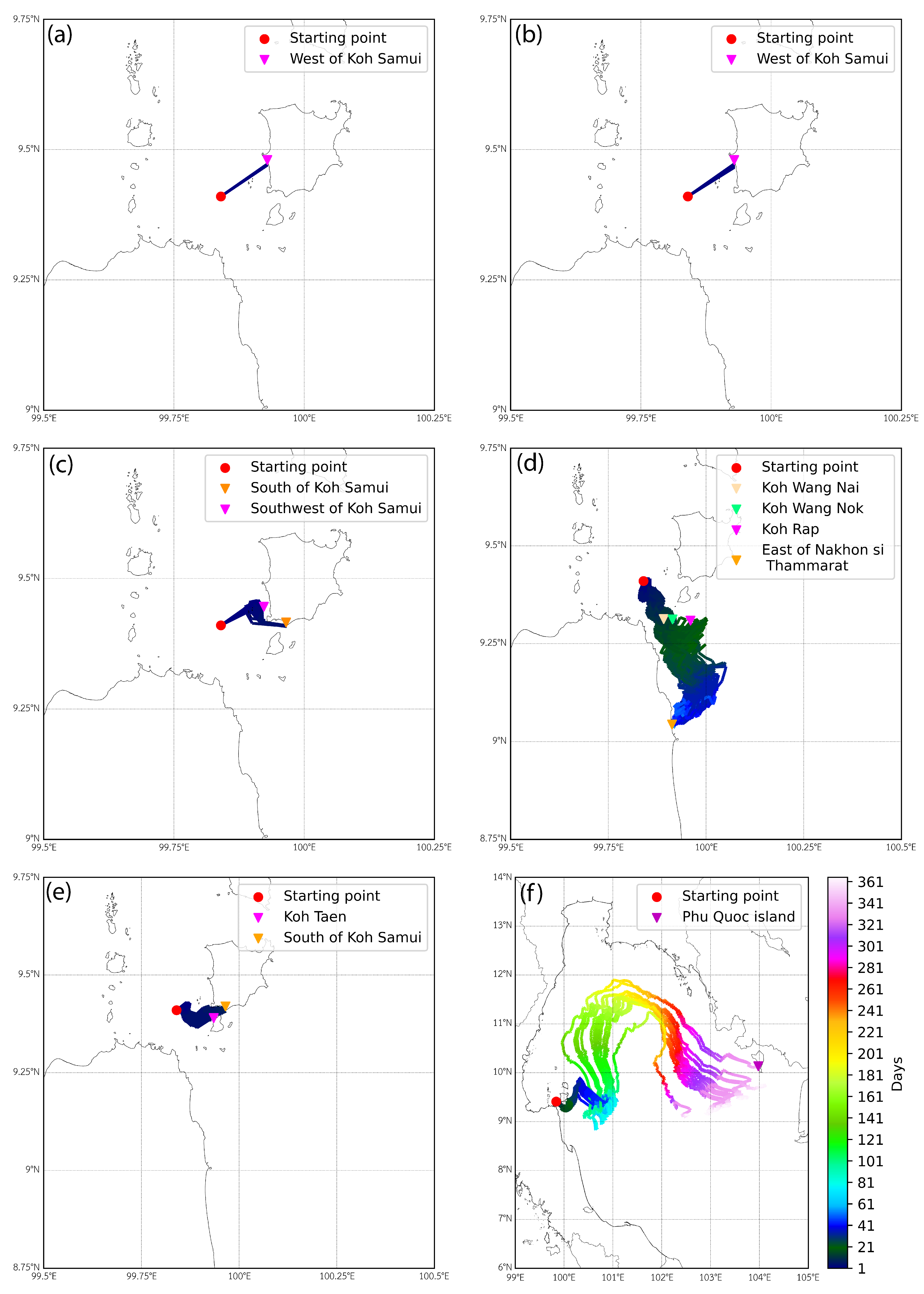
3.2. Marine Debris’s Path

The movement of marine debris from the LPT model is calculated by using the current velocity from the OCM, wind velocity at 10 m, and random walk term with the buoyancy ratios in six cases, which are 100:1, 10:1, 1:1, 0:1, 1:10, and 1:100 (Figure 4). We simulate the path of marine debris with a case study; the garbage boat capsized at 99.84${}^{\circ }\mathrm{E}$ and 9.41${}^{\circ }\mathrm{N}$ (starting point) from 1 August 2020 to 1 August 2021 (Figure 10).

The marine debris with a buoyancy ratio of 100:1 (refers to the plastic bottle [13] floating in the sea) moves northeastward from the starting point to the west coast of Koh Samui for 1–2 days (Figure 10a). The marine debris with a buoyancy ratio of 10:1 (refers to the plastic container [13] floating in the sea) moves northeastward from the starting point to the west coast of Koh Samui for 1–2 days (Figure 10b). The marine debris with a buoyancy ratio of 1:1 (refers to the marine debris floating on the sea and the cross-sections to the wind direction below and above the sea surface half each) moves northeastward from the starting point to the southwest coast and then moves eastward to the south coast of Koh Samui for 1–5 days (Figure 10c). The marine debris with a buoyancy ratio of 0:1 (refers to the marine debris floating under the sea surface, and it has no wind that affects the surface of marine debris) moves southward from the starting point to the Koh Wang Nai, Koh Wang Nok, and Koh Rap for 15–30 days and then moves to the east coast of Nakhon Si Thammarat province for 30–55 days (Figure 10d). The marine debris with a buoyancy ratio of 1:10 (refers to the marine debris floating on the sea surface, the marine debris has sea surface currents and wind that affect the surface of marine debris) moves eastward from the starting point to the Koh Taen and south of Koh Samui for 3–5 days (Figure 10e).The marine debris with a buoyancy ratio of 1:100 (refers to the marine debris floating on the sea surface, the marine debris has sea surface currents and wind that affect the surface of marine debris) moves southward from the starting point to the Koh Taen for 3–5 days, Ko Rap for 15–20 days and then moves northeastward to the southeast of Koh Samui for 25–30 days. Moreover, marine debris moves eastward to the Phu Quoc island in Vietnam and the middle and east of the GoT for one year (Figure 10f).

4. Conclusions

The marine debris path is simulated by using the OCM and LPT model; the OCM based on the SWE is used to calculate current velocity and sea surface elevation using meteorological data (wind velocity at 10 m and surface pressure). The SWE are solved by the finite difference method with Arakawa C-grid and splitting methods. The mean current velocity from the OCM is compared with the mean surface current of OSCAR; the result of the OCM reveals the eddy and direction of current velocity similar to the mean surface current of OSCAR. We compare the u-velocity and v-velocity between the OCM and OSCAR using RMSE. The RMSE of u-velocity is 0.070 m/s and that of the v-velocity is 0.058 m/s. From the LPT model, the controllable and uncontrollable factor is considered by current velocity from the OCM, wind velocity, random walk, and buoyancy ratio. The buoyancy ratio with six cases (100:1, 10:1, 1:1, 0:1, 1:10, and 1:100) considers the garbage boat that capsized on 1 August 2020 at 99.84${}^{\circ }\mathrm{E}$ and 9.41${}^{\circ }\mathrm{N}$ as a case study. The simulation shows that marine debris from the starting point moves to Koh Samui, Koh Taen, Koh Wang Nai, Koh Wang Nok, Koh Rap, the east coast of Nakorn Si Thammarat province, Phu Quoc Island of Vietnam and the middle of the GoT with the various buoyancy ratios and time duration. The closest movement of marine debris from the starting point was on the west coast of Koh Samui with a buoyancy ratio of 100:1, 10:1, and 1:1, and the furthest movement of marine debris from the starting point was on the Phu Quoc island in Vietnam with a buoyancy ratio of 1:100.

References

- Chanthamat, Y.; Israngkun Na Ayutthaya, A. Marine Garbage, the National Plan Must Not Neglect the Community. 2021. Available online: https://tdri.or.th/2021/06/worldoceanday/ (accessed on 7 April 2021).
- Abolfathi, S.; Cook, S.; Yeganeh-Bakhtiary, A.; Borzooei, S.; Pearson, J. Microplastics Transport and Mixing Mechanisms in The Nearshore Region. Coast. Eng. Proc. 2020, 36, 63. [Google Scholar] [CrossRef]
- Abolfathi, S.; Pearson, J. Solute Dispersion in The Nearshore due to Oblique Waves. Coast. Eng. Proc. 2014, 1, 49. [Google Scholar] [CrossRef] [Green Version]
- Abolfathi, S.; Pearson, J. Application of Smoothed Particle Hydrodynamic (SPH) in Nearshore Mixing: A Comparison to Laboratory Data. Coast. Eng. Proc. 2017, 35, 16. [Google Scholar] [CrossRef]
- Ren, Z.Y.; Zhao, X.; Wang, B.L.; Dias, F.; Liu, H. Characteristics of wave amplitude and currents in South China Sea induced by a virtual extreme tsunami. J. Hydrodyn. 2017, 29, 377–392. [Google Scholar] [CrossRef]
- Ren, Z.; Liu, H.; Jimenez, C.; Wang, Y. Tsunami resonance and standing waves in the South China Sea. Ocean. Eng. 2022, 262, 112323. [Google Scholar] [CrossRef]
- Guo, D.; Zeng, Q.; Ji, Z. A Numerical model of Storm Surges and Its Open Boundary Problems. Chin. J. Atmos. Sci. 1992, 16, 193–204. [Google Scholar]
- Collins, S.; James, R.; Ray, P.; Chen, K.; Lassman, A.; Brownlee, J. Grids in Numerical Weather and Climate Models. Clim. Chang. Reg. Responses 2013, 256, 111–128. [Google Scholar]
- Aschariyaphotha, N.; Wongwises, P.; Wongwises, S.; Humphries, U.W.; You, X. Simulation of seasonal circulations and thermohaline variabilities in the Gulf of Thailand. Adv. Atmos. Sci. 2008, 25, 489–506. [Google Scholar] [CrossRef]
- Carlson, D.F.; Suaria, G.; Aliani, S.; Fredj, E.; Fortibuoni, T.; Griffa, A.; Russo, A.; Melli, V. Combining Litter Observations with a Regional Ocean Model to Identify Sources and Sinks of Floating Debris in a Semi-enclosed Basin: The Adriatic Sea. Front. Mar. Sci. 2017, 4, 78. [Google Scholar] [CrossRef] [Green Version]
- Seo, S.; Park, Y.G.; Kim, K. Destination of floating plastic debris released from ten major rivers around the Korean Peninsula. Environ. Int. 2020, 138, 105665. [Google Scholar] [CrossRef] [PubMed]
- Seo, S.; Park, Y.G.; Kim, K. Tracking flood debris using satellite-derived ocean color and particle-tracking modeling. Mar. Pollut. Bull. 2020, 161, 111828. [Google Scholar] [CrossRef] [PubMed]
- Yoon, J.-H.; Kawano, S.; Igawa, S. Modeling of marine litter drift and beaching in the Japan Sea. Mar. Pollut. Bull. 2010, 60, 448–463. [Google Scholar] [CrossRef] [PubMed]
- Aongponyoskun, M. The Diffusion Coefficient of Seawater in Ao Si Racha. Kasetsart J. Nat. Sci. 2008, 42, 49–53. [Google Scholar]
Publisher’s Note: MDPI stays neutral with regard to jurisdictional claims in published maps and institutional affiliations. |
© 2022 by the authors. Licensee MDPI, Basel, Switzerland. This article is an open access article distributed under the terms and conditions of the Creative Commons Attribution (CC BY) license (https://creativecommons.org/licenses/by/4.0/).
Share and Cite
Phiphit, J.; Wangwongchai, A.; Humphries, U.W. Simulation of Marine Debris Path Using Mathematical Model in the Gulf of Thailand. Axioms 2022, 11, 571. https://doi.org/10.3390/axioms11100571
Phiphit J, Wangwongchai A, Humphries UW. Simulation of Marine Debris Path Using Mathematical Model in the Gulf of Thailand. Axioms. 2022; 11(10):571. https://doi.org/10.3390/axioms11100571
Chicago/Turabian StylePhiphit, Jettapol, Angkool Wangwongchai, and Usa Wannasingha Humphries. 2022. "Simulation of Marine Debris Path Using Mathematical Model in the Gulf of Thailand" Axioms 11, no. 10: 571. https://doi.org/10.3390/axioms11100571