1. Introduction
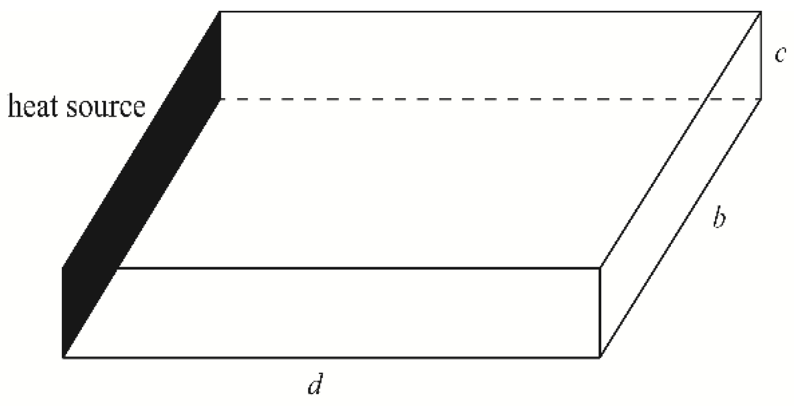
Joseph Fourier studied the temperature variation of a rod with an infinite length and adiabatic surface [
1]. Its initial temperature is 0 °C, and the temperature remains constant with one end heated. This forms a 1D heat conduction model under Dirichlet boundary conditions in a semi-infinite domain, which has become one of the most classical heat conduction problems [
2]. Current solving methods of heat conduction problems mainly include analytical and numerical methods. With the vigorous development of computer technology, the numerical method has now become the main calculation method in scientific research and engineering design [
3,
4,
5,
6,
7], and the importance of an analytical solution is usually neglected. Actually, the analytical method is an important tool in the study of mathematical physics models, exhibiting the advantages of clear physical concepts, distinct physical meaning, and a reliable theoretical basis [
8]. The analytical solution not only reveals the intrinsic mechanism and mathematical laws of heat conduction problems, but also provides an effective means to test the applicability and correctness of the numerical method, since the analytical solution can be approximated as an exact solution under specific boundary conditions [
9]. In previous research, the function of boundary temperature,
f(
t) is often given with a relatively simple specific expression. Hence, many methods have been proposed to obtain analytical solutions to models for practical engineering problems basing on heat conduction equations, such as groundwater seepage [
10,
11], contaminant transport [
12,
13], and geothermal field research [
14,
15,
16], especially using integral methods, as well as some new methods based on them. For example, we cite Laplace transform [
17], Fourier transform [
18], a new iteration method [
19], an approximate analytical integral method [
20], an integral-balance method [
21], and a boundary integral method [
22].
However, in real-world applications, the process of the variation of boundary temperature is sometimes complex, and it is difficult to provide a specific and accurate expression for its corresponding function
f(
t). For example, in a test involving the control of a material temperature field through the Dirichlet boundary, continuous manual intervention is required to effectively control the temperature variation of the tested material. Consequently,
f(
t) is a complex and random function of time. In this case, theoretical solutions of 1D heat conduction models in the semi-infinite domain can be obtained by utilizing certain specific properties of the integral transform. During the research of heat conduction problems with a linear heat source, Wu utilized the convolution and differential properties of the Laplace transform to provide the general theoretical solution of the model [
16]. Nevertheless, the calculation process is complicated, and the given solution is complex in form and inconvenient to apply. Moreover, considering the complexity and variability of boundary conditions, some studies have examined the influence of boundary conditions on the solving process of the model and the handling of boundaries in specific problems [
23,
24]. When
f(
t) changes slowly, the sectional equivalence discrete method can be applied to solve the model based on the basic solution of the classical model [
25]. However, this discrete method is unable to reveal the cumulative impact of changing boundary conditions within a specific period.
The aim of this paper is to propose a shortcut method to derive the analytical solution for a 1D heat conduction model in a semi-infinite space under the condition that the variation process of boundary temperature is complicated. Based on properties of the Fourier transform, the theoretical solution for the model is given, which is composed of commonly used functions with a relatively simple form. Subsequently, the piecewise linear interpolation function of f(t) established by temperature measurements is directly substituted into the theoretical solution to obtain the corresponding analytical solution. This method avoids the tedious deduction process; thus, the calculation process is relatively brief and easy to apply in practice. Additionally, the cumulative effect of boundary conditions can be reflected. This method of resolution can also be applied for research regarding porous media seepage and pollutant diffusion using similar models.
An important application of the derived analytical solution to the problem is to calculate thermal diffusivity by the measured temperature data. The thermal diffusivity of soil is a key element in the design of borehole heat exchangers in ground source heat pump systems [
26], which reflects the variation rate of soil temperature with time. In recent years, the methods for gaining thermal diffusivity have often been divided into two categories: one is estimation based on in situ temperature records, such as infrared thermal imaging [
27], photothermal beam deflection spectroscopy [
28], and the Fourier spectroscopy method [
29], and the other is prediction by building models, including infinite line source models [
30] and semi-empirical models [
31]. However, the thermal diffusivity obtained by the above methods is either estimated, or the solving process is complicated. Therefore, we propose a simple and relatively accurate method for solving the thermal diffusivity based on the analytical solution by combining the measured temperature data.
4. Methods
Based on temperature data obtained in the experiment, the analytical solution of the heat conduction model under the linear decay function boundary condition is applied to solve for the thermal diffusivity of soil by using principles of the inflection point method and the curve fitting method.
4.1. Curve Fitting Method
The curve fitting method is a simple and convenient method for parameter estimation, avoiding the systematic calculation errors caused by traditional parameter estimation methods, such as the traditional moment method and the maximum likelihood method; thus, it is widely used in the field of hydrogeology [
35]. For a temperature measurement point at distance
x from the boundary, where the value of
x is fixed,
φt(
x,t) can be calculated for different values of
a at different moments
t by Equation (23), from which a family of theoretical curves corresponding to different
a values,
φt(
x,t) −
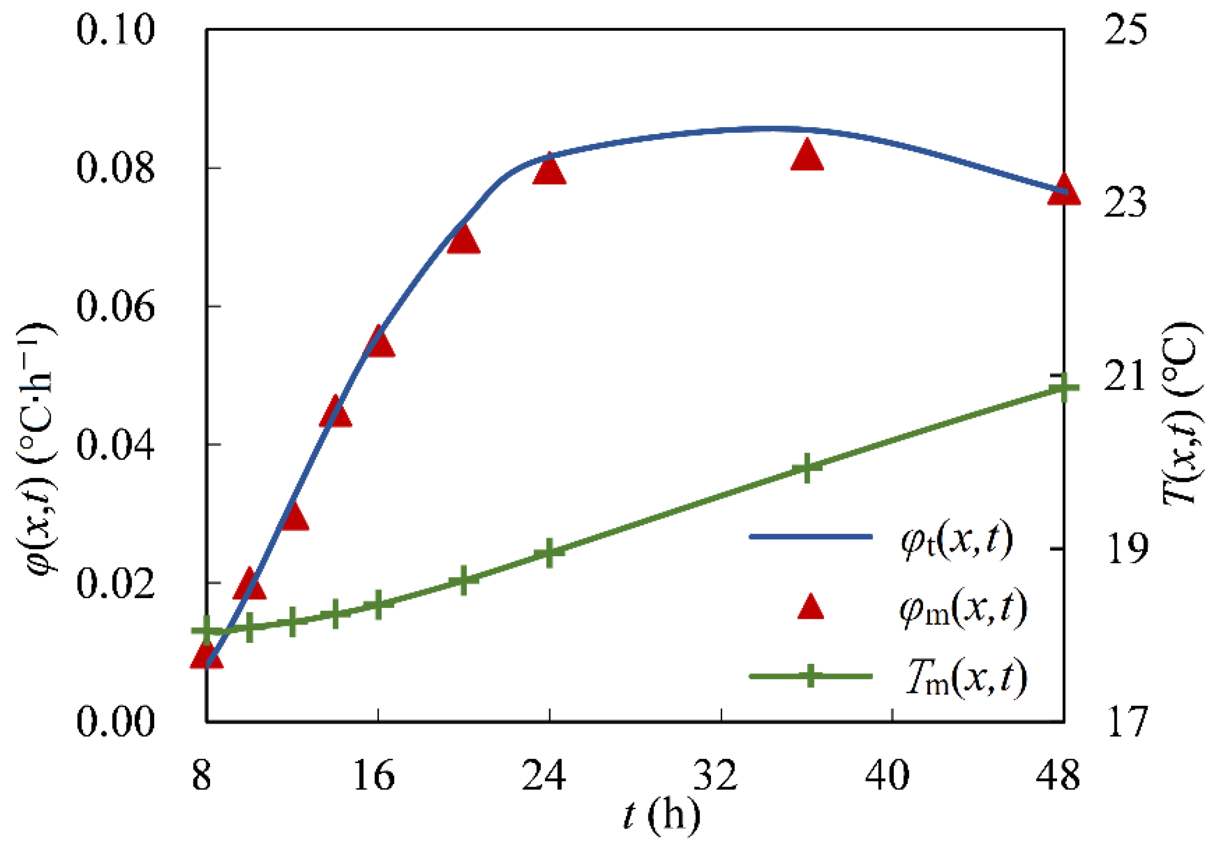
t can be drawn. Meanwhile, from the measured data at the temperature measurement point, the measured temperature variation rate curve,
φm(
x,t) −
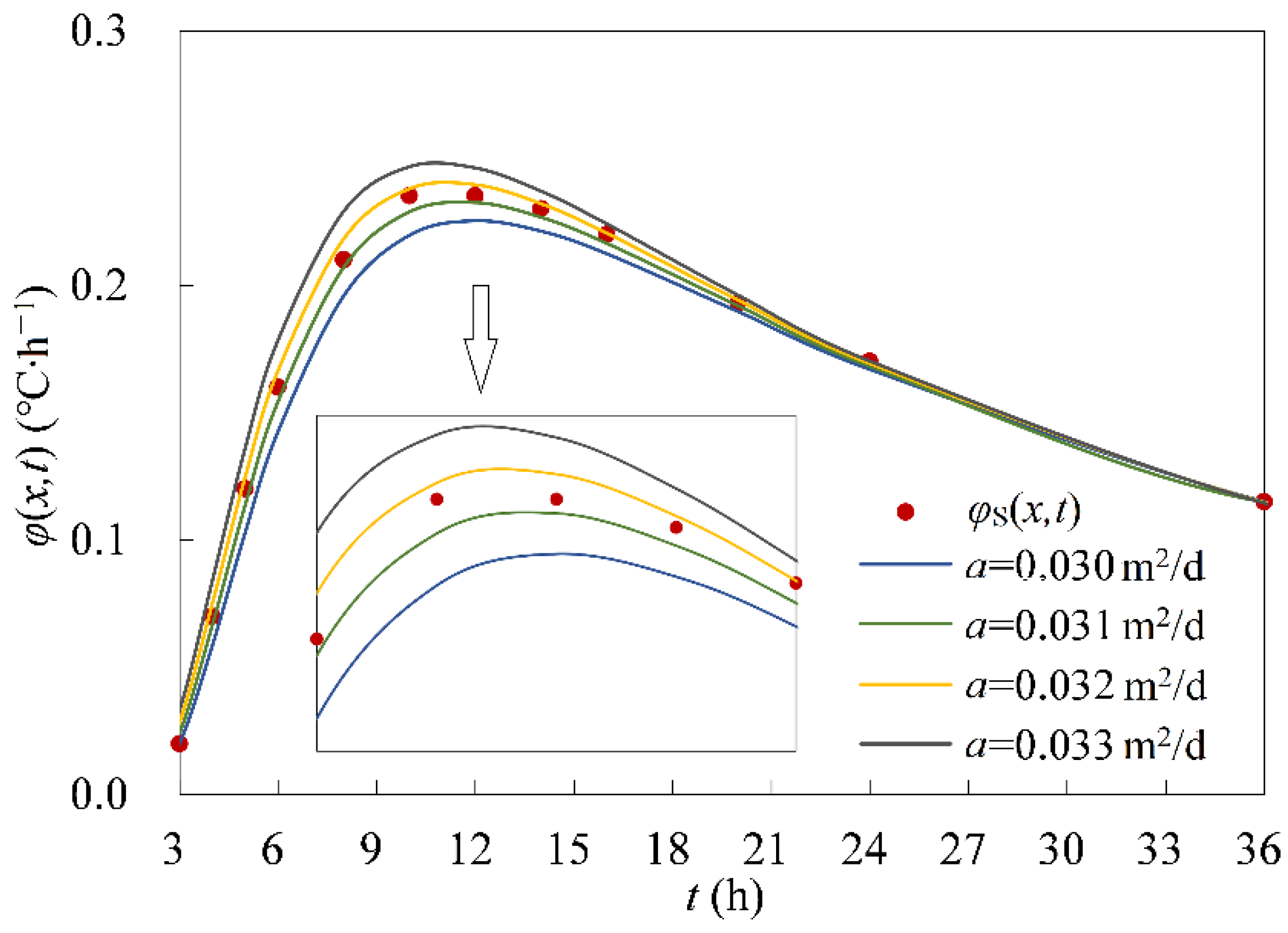
t can be drawn.
When the value of a in the φm(x,t) − t curve is identical to that of a curve in the φt(x,t) − t theoretical family, the two curves should have the same shape and overlap exactly. According to this principle, the value of a in the specimen can be determined by the curve-fitting process of the measured φm(x,t) − t curve and the theoretical φt(x,t) − t curve family.
4.2. Inflection Point Method
The inflection point method is a method of plotting curves according to actual measurement data and using its inflection point to graphically solve for parameters [
36]; this method is widely applied in many fields, including civil engineering, chemistry, and hydrogeology.
According to Equation (23), we have
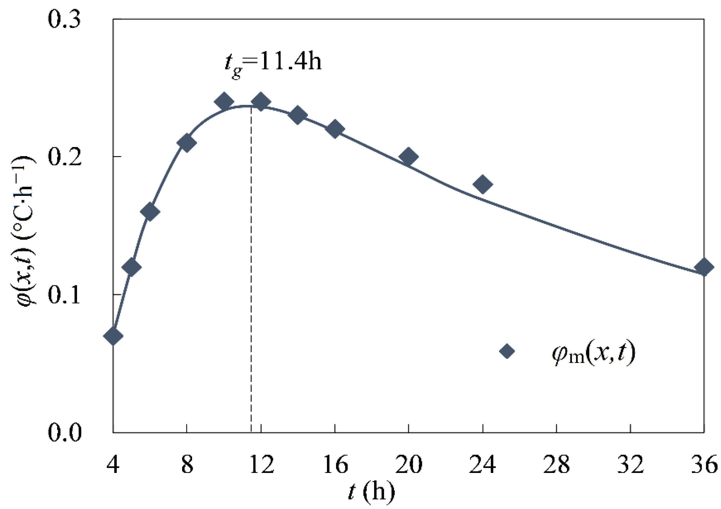
It can be seen from Equation (24) that an inflection points exist on the
φ(
x,t)
− t curve. Let us denote the time corresponding to inflection points as
tg, which can be calculated by
tg = 0 as
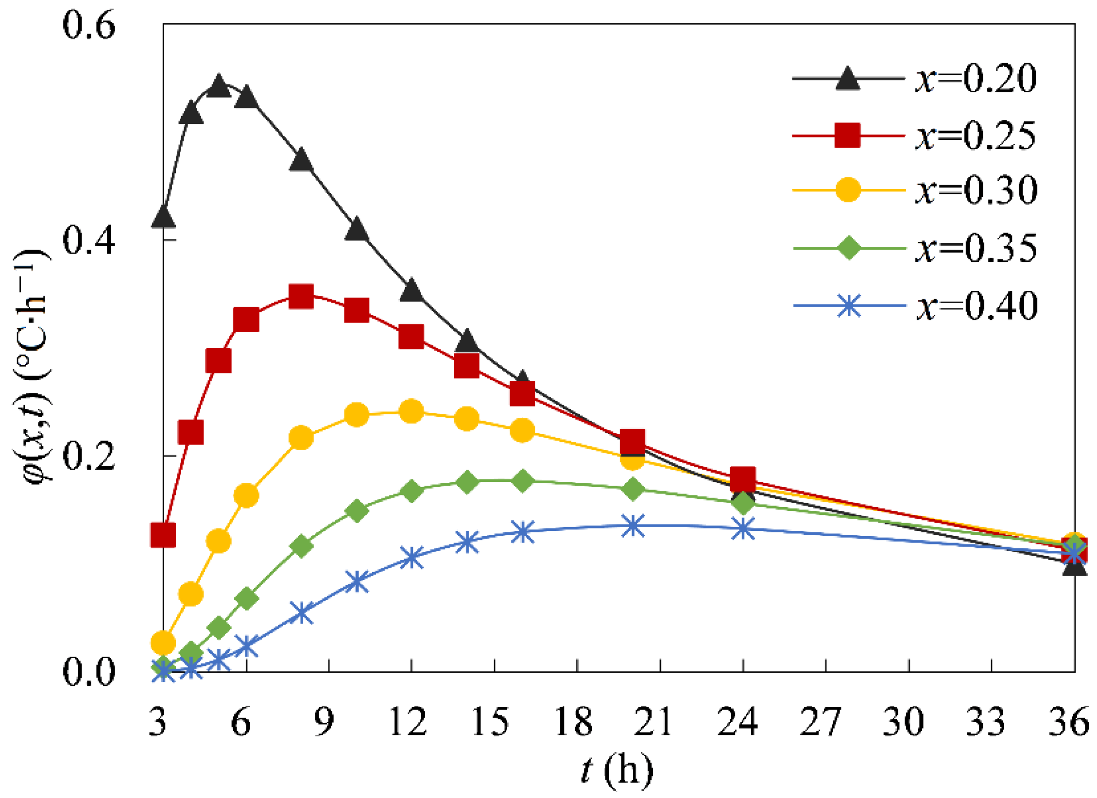
When the value of x is fixed, the variation process of φ(x,t) with time can be drawn as the φ(x,t) − t curve.
It should be noted that, regardless of the positive or negative of β, under the boundary condition, which is a monotonic function with ΔT0 and β as fixed values, there cannot be two inflection points on the φ(x,t) − t curve at any point. That is, only one of the Equations (25) and (26) regarding tg is reasonable. From Equation (26), when β < 0, tg < 0, this is not consistent with the physical meaning of the problem, i.e., Equation (26) is not universal. The calculation result of Equation (25) does not produce the above contradiction, i.e., Equation (25) is universal.
According to the inflection point tg of the measured φ(x,t) − t curve, the model parameter a can be calculated from Equation (25), when combined with the measured ΔT0, β, and x in the test.


