1. Introduction
The bi-dimensional Fuzzy Transform (F-transform) has been initially proposed in [
1] as a lossy image compression technique. The direct F-transform is applied to construct the compressed image and the image is reconstructed by computing the inverse F-transform. In [
2,
3], the image is partitioned in blocks and the F-transform technique is applied to compress each block. In [
2], the authors show that the F-transform image compression technique applied to blocks of the image achieves the best performance with respect to the images in which fuzzy relation equations are applied. In [
3,
4], the authors compare the F-transform and JPEG image compression technique, showing that the two methods provide similar results in terms of decompressed image quality, but F-transform has shorter execution times than JPEG.
In the last decade, the bi-dimensional F-transform has been applied in various image processing problems, such as image fusion [
5,
6,
7], image autofocus [
8,
9], edge detection [
10,
11], image segmentation [
12,
13], image watermarking [
14], and noise reduction [
15]. An overview of the main image processing techniques that use the two-dimensional F-transform is provided in [
16].
To control the loss of information due to the compression, the authors of [
17] proposed a variation of the F-transform method called Multilevel F-transform (MF-tr), in which the image is compressed hierarchically in a multilevel structure similar to the ones used in Laplace Pyramid [
18] and Wavelet-based [
19,
20] image compression. Initially, the image is compressed using the two-dimensional block-based F-transform method. It is subsequently decompressed, and the quality of the decompressed image compared to the original image is measured, computing the Peak Signal to Noise Ratio index (PSNR). If the quality of the decompressed image is lower than a predetermined threshold, the “Error” image is constructed, which is provided by the difference between the original image and the decompressed one, and the two-dimensional F-Transform is applied to compress the Error image. The reconstruction image will consist of the previously decompressed image in addition to the decompressed image of the Error. The PSNR of the reconstructed image is computed with respect to the original image; if the PSNR is below the threshold, the new Error image is built and the process is iterated into the next level. The process ends when the PSNR of the reconstructed image with respect to the original image is greater than or equal to the threshold.
The final reconstructed image is given by the sum of all reconstructed images computed in each level. This method represents a trade-off between the reconstructed image quality and the compression rate. If it is necessary to obtain a high quality of the reconstructed image, with a minimum loss of information compared to the original image, then a high value of the PSNR threshold is set and the execution times will be longer.
In [
21], a variation of MF-tr, called Fast Multilevel Fuzzy Transform (Fast M-ftr), is proposed to accelerate execution times. In Fast M-ftr, a preprocessing phase is performed to find the optimal value of the compression rate, which guarantees to minimize the number of iterations.
The bi-dimensional F-transform can be applied to compress high resolution images. The authors of [
22] compared four satellite lossy image compression methods using the wavelet domain, which are the image compression algorithm proposed by the Consultative Committee for Space Data Systems (CCSDS) [
23], Wavelet lossy image compression [
24], Bandelet [
25], and JPEG 2000 [
26]. The authors show that the CCSDS has the highest resolution image compression.
In [
27], the authors use pseudo-exponential functions as basic functions. They compare the results with the ones obtained by applying the F-transform with cosinusoidal basic functions and wavelet image compression methods, showing that the decompressed images obtained with their method have high quality, but also high time consumption.
A hybrid massive image compression method is proposed in [
28]. The bi-dimensional F-transform is used to compress the original image. Then, adjoint pixels in the compressed image with the same gray level are binned by merging them in a bin.
This method is very effective in the lossy compression of massive images, where it is not necessary to limit or reduce the information loss. In addition, the binning of images compressed via the bi-dimensional F-transform is a good trade-off between the level of compression and the quality of the reconstructed image.
In some cases, as in high level medical and remote sensing images, it is necessary to check that the quality of the decompressed image remains above a prefixed threshold. The F-transform massive image compression [
28] is unsuitable for checking that the quality of the decompressed image is always greater than the threshold, unlike the algorithms based on the bi-dimensional MF-tr [
17,
21].
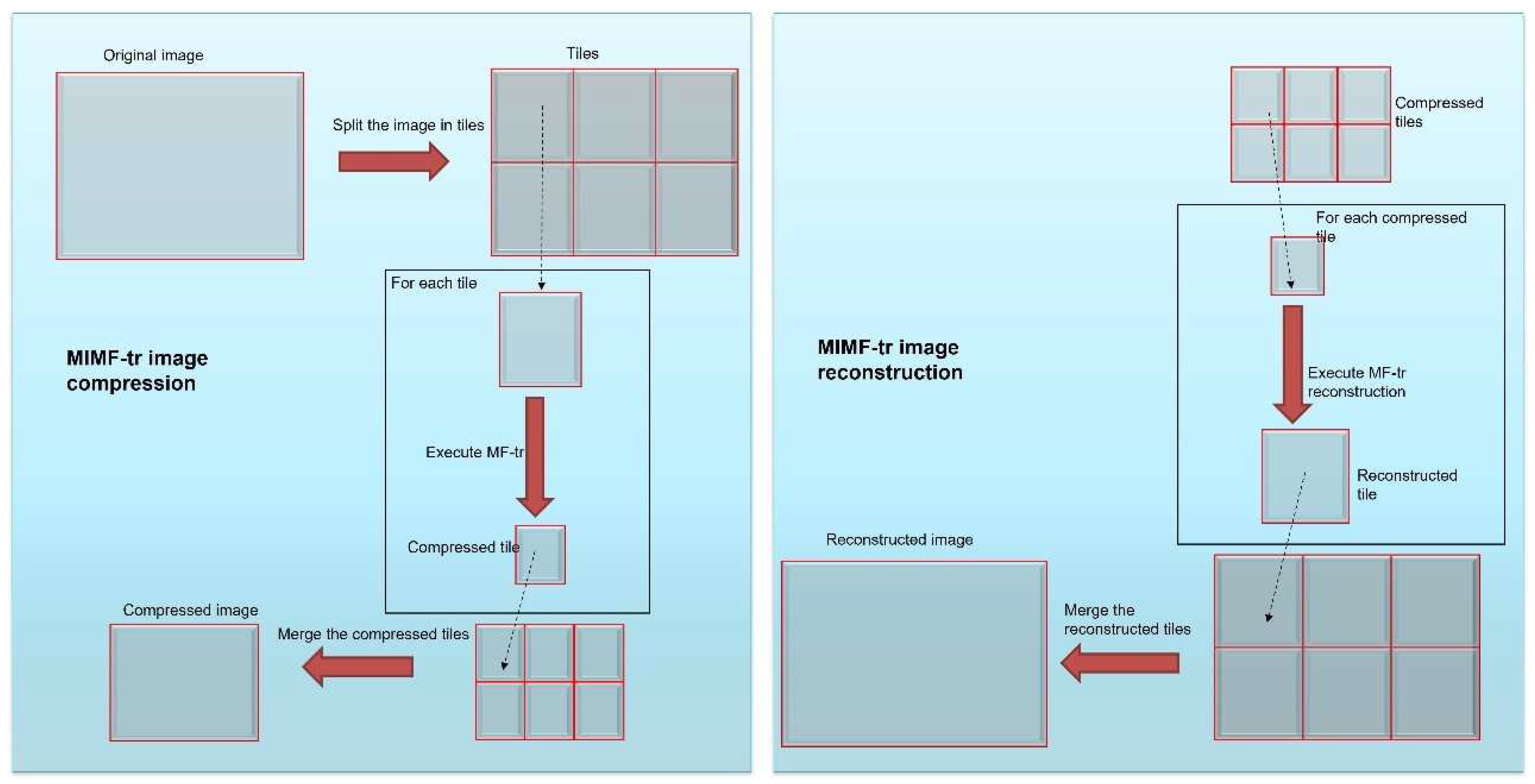
In this paper, we present a new approach based on the MF-tr to massive images. We call this method Massive Image Multilevel F-transform compression method (MIMF-tr). Our idea is to split the image into tiles of equal size. Splitting the image in tiles is necessary to compress massive images; each tile is compressed separately by executing the MF-tr compression algorithm. Then, all of the compressed tiles are merged to compose the compressed image. The decompressed image is obtained by executing the MF-tr image reconstruction method to each compressed tile and, finally, merging the reconstructed tiles.
MIMF-tr, similar to MF-tr, allows for controlling the quality of the compressed image. Furthermore, unlike MF-tr, MIMF-tr is suitable for compressing massive images, adopting a technique of partitioning the image in tiles and compressing the tiles separately.
In
Figure 1, the MIMF-tr image compression and reconstruction methods are schematized.
The Peak Signal to Noise Ratio (PSNR) measure is used to measure the quality of the compression. Each tile is partitioned in blocks and each block is compressed using the MF-tr compression method, in which the iteration process with the execution of the subsequent level continues until the PSNR of the decompressed block is greater than or equal to a fixed threshold.
In
Section 2, we briefly describe the base concepts of direct and inverse F-transform and discuss the MF-tr image compression and reconstruction algorithms. In
Section 3, we present the MIMF-tr image compression and reconstruction algorithms. The results of comparison tests executed on massive images are shown in
Section 4. Conclusions are included in
Section 5.
2. Preliminaries
2.1. Discrete Direct and Inverse F-Transform for Coding/Decoding Images
The bi-dimensional discrete F-transform was applied in [
1,
2,
3] for coding/decoding a gray level image by approximating a continuous function
f: X → Y in a closed interval [a,b] based on the knowledge of the value of
f in a discrete set of points.
In [
1], the concept of basic functions is introduced, which is given by the fuzzy set of a fuzzy partition of a closed interval real domain [a,b], as described below.
Let {x1, x2, …, xn} be a set of n ≥ 2 points of [a,b], called nodes, in order that x1 = a < x2 <…< xn = b. A fuzzy partition of [a,b] is given by a family of fuzzy sets A1,…,An: [a,b] → [0,1], where Ai(x), i = 1,2,…,n, are continuous functions on [a,b] if the following conditions hold:
Ai(xi) = 1, ∀ i ∈ {1,2,…,n};
Ai(x) = 0 ∀ x ∉ (xi−1, xi+1), where we assume x0 = x1 = a and xn+1 = xn = b;
Ai(x) strictly increases on [xi−1, xi], ∀ x ∈ [a,b], and ∀ i ∈ {1,2,…,n};
Ai(x) strictly decreases on [xi, xi+1], ∀ x ∈ [a,b], and ∀ i ∈ {1,2,…,n−1};
Let f be a continuous function defined in [a,b]. Furthermore, let P = { p1,...,pN } be a set of N points in [a,b], where the values assumed by the function f are known. The set P is called a set of points, which is sufficiently dense with respect to the fuzzy partition {A1, A2,…, An} if for each basic function Ai, i = 1,…,n, exists in at least a point pj, j = 1,…,m, in order that Ai(pj) > 0.
If P is sufficiently dense with respect to the fuzzy partition {A
1, A
2,…, A
n}, we can define the n-dimensional vector
F = [F
1, …,F
n] with components:
called discrete direct F-transform of
f with respect to the fuzzy partition {A
1, A
2,…, A
n}.
The value of
f in a point x ∈ [a,b] can be approximated using the discrete inverse F-transform of
f with respect to {A
1, A
2, …, A
n}, given by the formula:
Now, let I be an N×M image. The previous concept of direct and inverse F-transform of a function defined on a real closed interval [a,b], can be extended to two-variable functions defined in the closed interval [a,b] × [c,d]. In this case, we can consider the image I as a bi-dimensional function defined on the closed interval [1,N] × [1,M], known in all the points with coordinates (i,j) of the pixels, where i ∈ [1,N] and j ∈ [1,M].
Furthermore, let A
1, …, A
n: [1,N] → [0,1] be a fuzzy partition of [1,N] and B
1, …, B
m: [1,M] → [0,1] be a fuzzy partition of [1,M]. Clearly, the sets of points P={1,2, …, N} and Q={1,2, …, M} are sufficiently dense with respect to the partitions {A
1, A
2, …, A
n} and {B
1, …, B
m}, respectively. Therefore, we can define the bi-dimensional discrete direct F-transform of
f given by the matrix
F with components:
The compressed n × m image is given by the direct F-transform F. The compression rate (the inverse of the compression ratio parameter) is .
The original image is reconstructed by computing the bi-dimensional discrete inverse F-transform with respect to {A
1, A
2, …, A
n} and {B
1, B
2, …, B
m} given by:
In [
2,
3,
4], the bi-dimensional discrete direct F-transform is applied to the compressed images.
2.2. Multilevel F-Transform for Massive Image Compression
The MF-transform image compression method is an F-transform based method that allows you to control the loss of information in compression phase.
Initially (Level 1), the source image is compressed using the bi-dimensional F-transform. Then, it is decompressed and the PSNR is measured and compared with the original image.
Formally, let I0 be the N × M source image. It is compressed using the direct bi-dimensional F-transform in an n × m image and it is decompressed using the inverse bi-dimensional F-transform in an N × M image . Call the image reconstructed at Level 1. At this level, we have , namely, the reconstructed image at the first level corresponds to the decompressed image.
The PSNR index is computed to measure the quality of the reconstructed image at each level. If the PSNR is greater than or equal to a prefixed threshold PSNRth the algorithm ends. Otherwise, a further image is calculated, called Error, whose pixels are given by the difference in absolute value between the corresponding pixels of the original image and those of the decompressed image.
The error image constitutes the input image to the next level (Level 2) . The previous process is repeated, obtaining the compressed image and decompressed image . The reconstructed image at this level is given by . If the PSNR of the reconstructed image measured with respect to the source image I0 is greater than or equal to PSNRth, then the process ends. Otherwise, the Level 2 error is calculated, which is given by the formula which represents the absolute difference between the source image at Level 2 and its decompressed image. The image is the source image in the input to the next level, Level 3.
This process continues iteratively until the PSNR of the reconstructed image at the level L, such as , measured with respect to the source image I0 is greater than or equal to PSNRth.
The PSNR of the image reconstructed at Level k is obtained by calculating the Mean Square Error (MSE) with respect to the source image I
0, given by:
The PSNR index is given by the formula:
where the parameter
GrLev is the number of gray levels of the source image.
The final reconstructed image is given by:
The pseudocode of the MF-tr image compression algorithm is shown below (Algorithm 1). It is executed by assigning the N × M source image I
0 as an input parameter, which is the compression rate ρ and the PSNR threshold PSNR
th.
| Algorithm 1 MF-tr image compression |
| Input: | N × M source image I0
Compression rate ρ
Threshold similarity PSNRth |
| Output: | Compressed n × m images obtained at each level |
| 1 | I:= |
| 2 | k:=1 |
| 3 | :=0 // is initialized to the Null N × M image |
| 4 | stopIter:=FALSE |
| 5 | PSNRold:=PSNRth |
| 6 | While (stopIter=FALSE) |
| 7 | :=DirectFTR(I,ρ) // Compression via direct F-transform |
| 8 | :=InversetFTR() // Decompression via inverse F-transform |
| 9 | := // Decompression via inverse F-transform |
| 10 | Calculate the PSNR index (6) |
| 11 | If (PSNR ≥ PSNRth) Then |
| 12 | stopIter:=TRUE |
| 13 | Else |
| 14 | k:=k+1 |
| 15 | |
| 16 | End If |
| 17 | End While |
| 18 | Return |
The reconstructed image is obtained by (7). In Algorithm 2, the image reconstruction algorithm is shown.
| Algorithm 2 MF-tr image reconstruction |
| Input: | n × m compressed images
Compression rate ρ |
| Output: | Reconstructed N × M image |
| 1 | : =0 // is initialized to the Null N × M image |
| 2 | For k = 1 to L |
| 3 | : =InversetFTR() // Decompression via inverse F-transform |
| 4 | : = |
| 5 | Next k |
| 6 | Return |
The compressed image will be constituted by L matrices with dimension n × m. The final compression rate will be given by:
3. The Massive Images Multilevel F-Transform Image Compression Method
The MF-tr technique is not suitable for handling massive images as it would require high CPU times and memory capacity. On the other hand, techniques for reducing the complexity of the image, such as the one proposed in [
28], are inapplicable if it is necessary to guarantee a minimum loss of information in the reconstructed image.
We propose a variation of the MF-tr technique in which the image is split in T tiles with an identical size. Each tile is separately compressed using the MF-tr method, with the constraint that the PSNR index of the reconstructed tile with respect to the original tile is not less than a prefixed threshold PSNRth.
Let I0 be a N0 × M0 massive image (for example, a remote sensing high resolution image in a band). The image I0 is split in T tiles with size N × M, where N = N0/T and M = M0/T. Each tile is separately compressed by executing the MF-tr compression method.
If I0t is the tth N × M tile, it will be compressed in a set of Lt n × m matrices where Lt is the number of levels needed to compress the tile I0t.
If
is the compression rate used to compress the N × M matrix at each level, the final compression rate is given by:
The mean final compression rate is
The MF-tr image compression algorithm (Algorithm 1) is used to reconstruct the original image. The correspondent function MF-trCompression() is called the MIMF-tr image reconstruction algorithm (Algorithm 3).
| Algorithm 3 MIMF-tr image compression |
| Input: | N0 × M0 source image I0
Compression rate ρ
Threshold similarity PSNRth |
| Output: | Compressed n × m images obtained at each level |
| 1 | Split the image in T tiles |
| 2 | For t = 1 to T |
| 3 | // Execute MF-trCompression() to compress the tth tile |
| 4 | : =MF-tr () |
| 5 | Next t |
| 6 | Return , , …, |
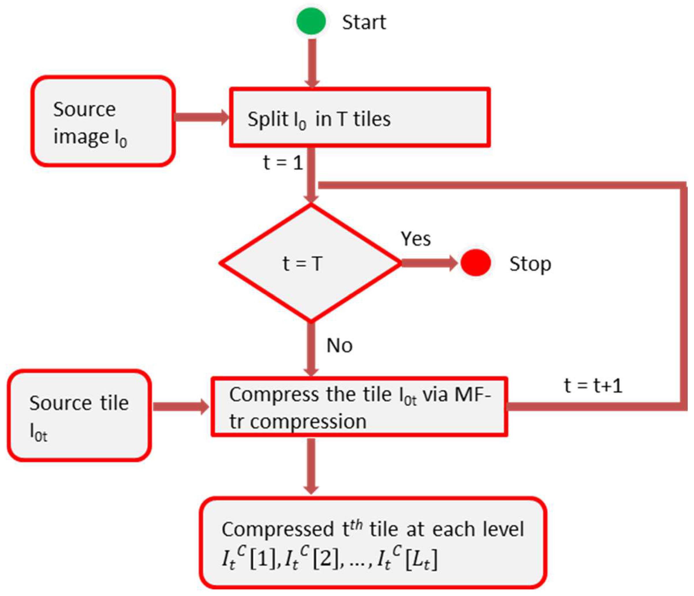
In
Figure 2, the flow diagram of the MIMF-tr image compression algorithm is schematized.
The MF-tr image reconstruction algorithm (Algorithm 2) is used to reconstruct the original image. The correspondent function MF-trReconstruction() is called in the MIMF-tr image reconstruction algorithm (Algorithm 4).
| Algorithm 4 MIMF-tr image reconstruction
|
| Input: | n × m compressed images
Compression rate ρ |
| Output: | Reconstructed N × M image |
| 1 | For t = 1 to T |
| 2 | // Execute MF-trReconstruction() to reconstruct the tth tile |
| 3 | =MF-tr() |
| 4 | Next t |
| 5 | : =merge ( |
| 6 | Return |
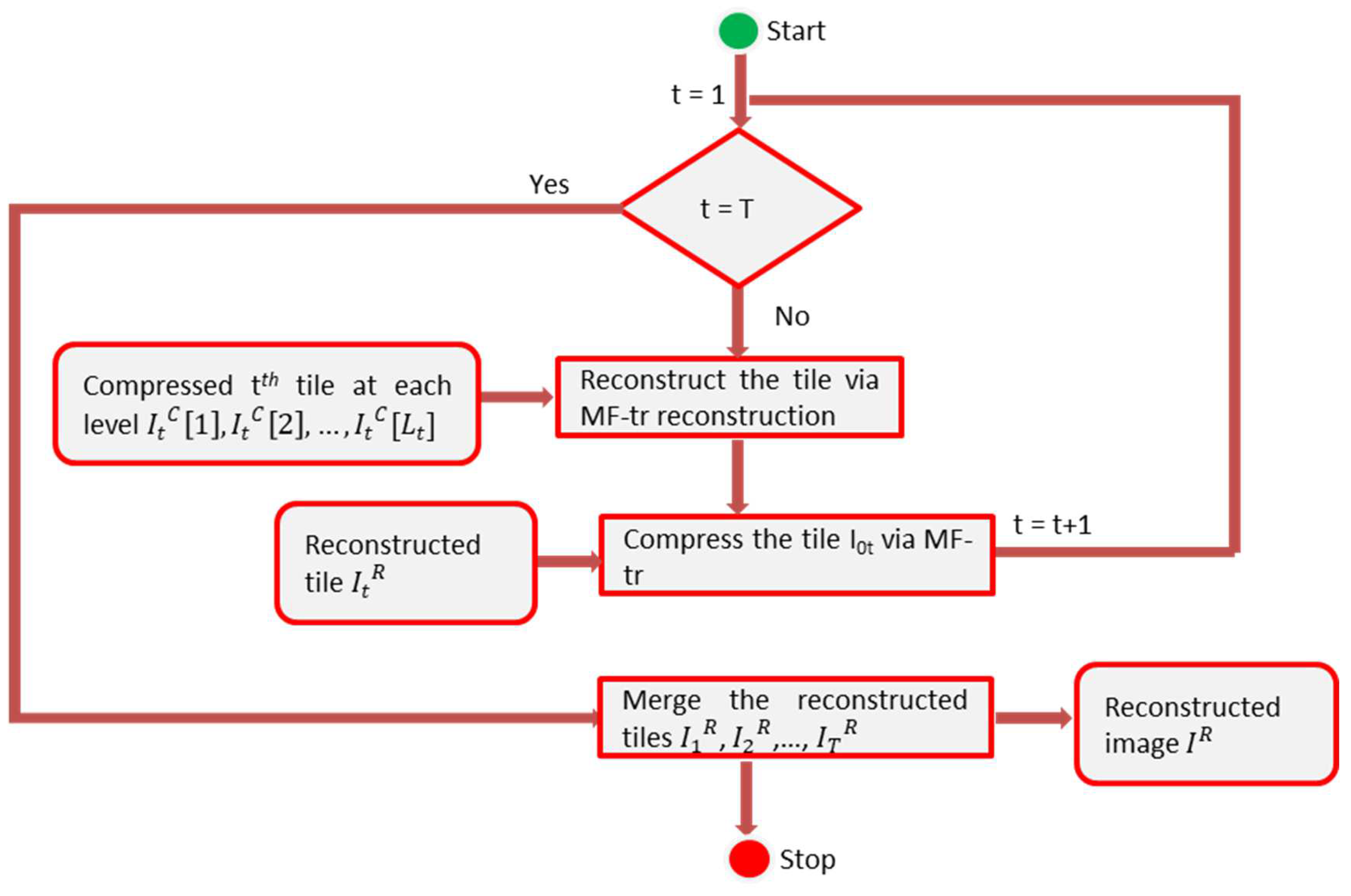
In
Figure 3, the flow diagram of the MIMF-tr image reconstruction algorithm is schematized.
The final PSNR index of the reconstructed image with respect to the original one is given by formula (6). The final compression rate, calculated by formula (10), varies according to the PSNR threshold and the complexity of the image; the higher the quality of the reconstructed image (i.e., intended to be guaranteed), the higher the average number of levels necessary in the compression, and the higher the final compression rate , the lower the compression of the image.
Since each tile is treated separately, the number of levels necessary in the compression can be different from tile to tile. If a tile contains more uniform or homogeneous image areas, the compression process will require the generation of fewer layers, compared to other tiles. A good choice of the number of tiles can be made in a way that some tiles can cover uniform image areas.
We test the MIMF-tr algorithm on a sample of remote sensing massive images by varying the number of tiles. To evaluate the best number of tiles in which we can split the image, we measure the mean number of levels necessary to compress the tiles given by:
We perform comparisons of our method with the MF-tr method measuring the final PSNR, the final compression rate, and the number of levels obtained by executing the two methods. In next section, we show and discuss the results of our tests.
4. Test Results
We test our method on a set of 200 HLS Landsat surface remote sensing images extracted from the NASA Earth Data website 3660 × 3660 pixels [
29]. The MIMF-tr algorithm was implemented in a Python platform; the tests were executed on an Intel Core i7-59360X processor with a clock frequency of 3 GHz. All the images are compressed with a compression rate ρ = 0.067. The threshold PSNR
th is set to 36.
We compare the performances of MIMF-tr with the ones of M-FTR in terms of number of levels necessary to compress the source images, final compression rate, and CPU time, using different values for the number of tiles in MIMF-tr. Briefly, we show in detail the results obtained for three images in the dataset.
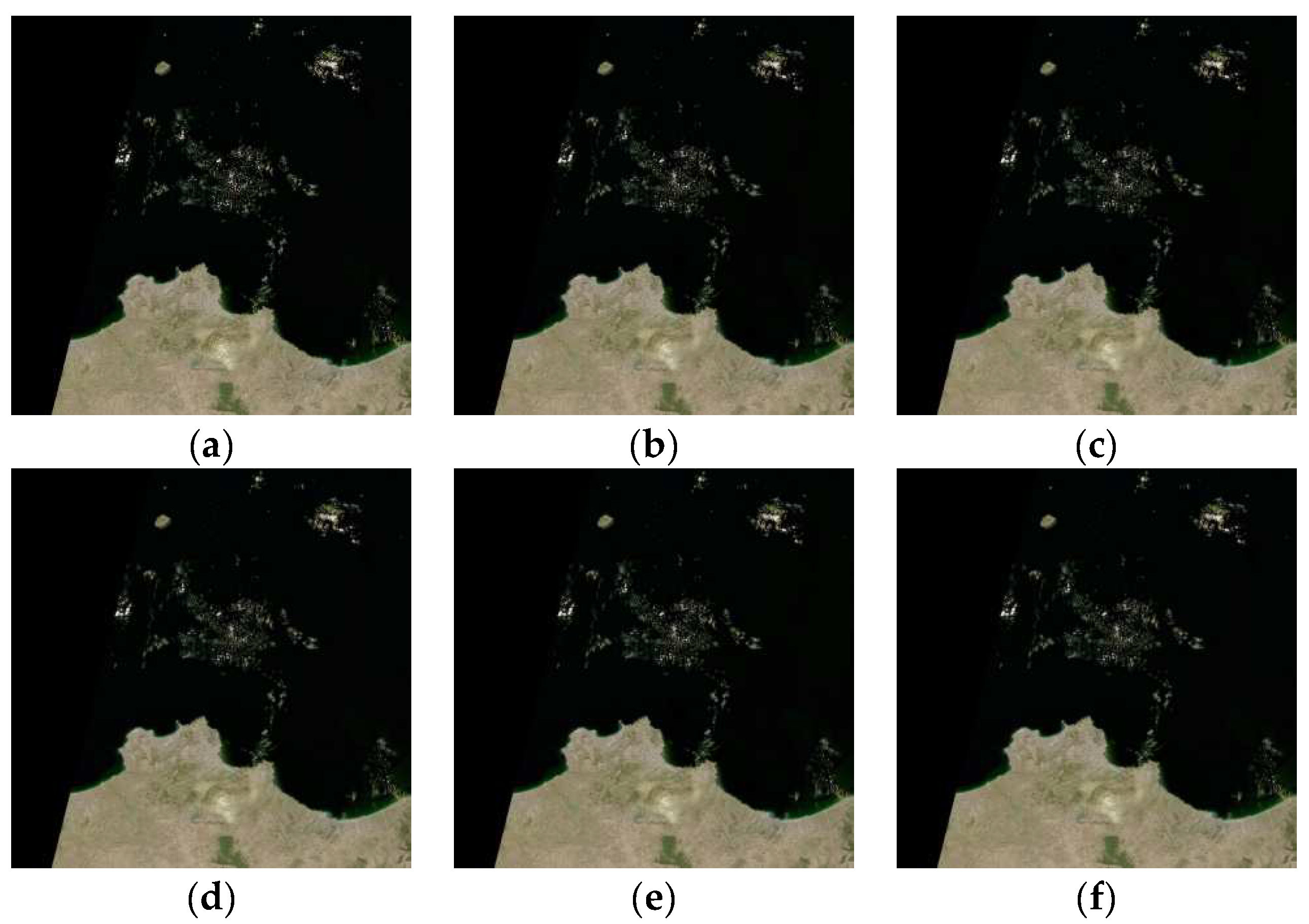
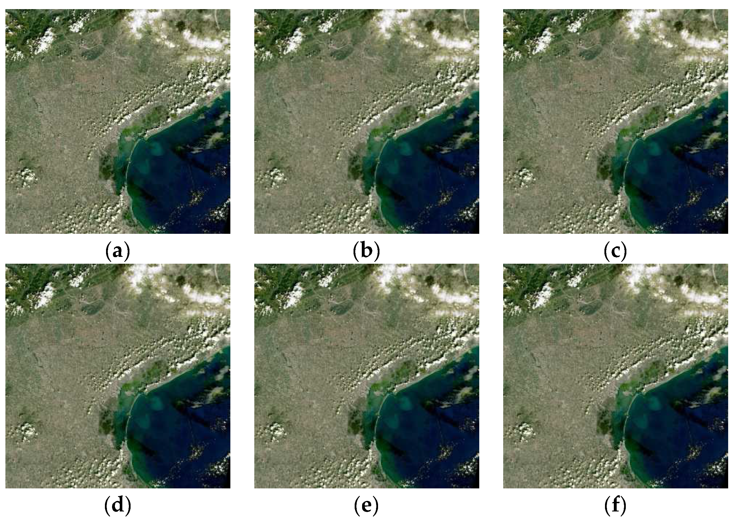
In
Figure 4a, the original image is shown, while in
Figure 4b, the reconstructed image obtained by executing MF-tr is shown.
Figure 4c–f shows the reconstructed images by splitting the original image in 6, 10, 20, and 30 tiles, respectively.
In
Table 1, the results obtained by compressing the satellite source image with MF-tr and MIMF-tr are shown in
Figure 4a. The mean level, PSNR, final compression rate, and CPU time are averaged on the three bands: Red, Green, and Blue.
The best results are obtained by MIMF-tr using 20 tiles. Furthermore, independently from the number of tiles set, the performances of MIMF-tr in terms of mean level, final compression rate, and CPU times obtained using MIMF-tr are better than the ones obtained using MF-tr. The final CPU time taken by MIMF-tr to compress the image is reduced by more than 23% compared to the CPU time taken by MF-tr. In addition, the mean number of levels achieved using MIMF-tr to obtain a reconstructed image with PSNR greater than 36 is always less than the one achieved using MF-tr. The final compression rate obtained executing MIMF-tr is always less than the final compression rate obtained by running MF-tr.
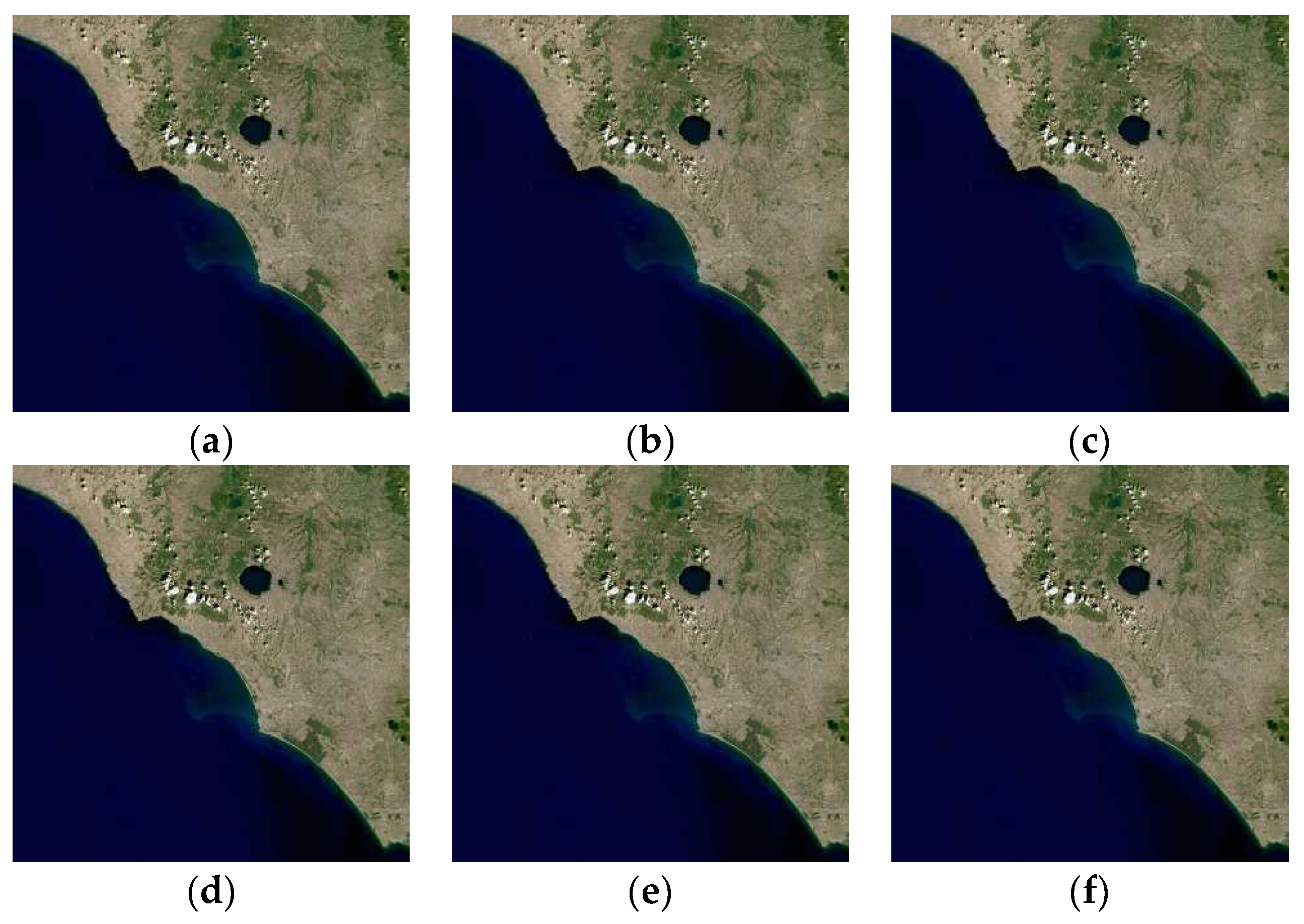
Figure 5a shows another HLS Landsat surface remote sensing image.
Figure 5b shows the reconstructed image obtained by executing MF-tr.
Figure 5c–f shows the reconstructed images by splitting the original image in 6, 10, 20, and 30 tiles, respectively.
In
Table 2, the results obtained by compressing the satellite source image in
Figure 5a with MF-tr and MIMF-tr are shown. The mean level, PSNR, and CPU time are averaged on the three bands: Red, Green, and Blue.
The best results are obtained by MIMF-tr using 10 tiles. As in the case of the previous image, the performances of MIMF-tr are better than the ones of MF-tr, independently from the number of tiles set. The CPU time taken by MIMF-tr to compress the image is reduced by more than 22% compared to the CPU time taken by MF-tr and the final compression rate and the mean number of levels are always less than the one measured using MF-tr.
Figure 6 shows another HLS Landsat surface remote sensing image.
Figure 5b shows the reconstructed image obtained by executing MF-tr.
Figure 5c–f shows the reconstructed images by splitting the original image in 6, 10, 20, and 30 tiles, respectively.
In
Table 3, the results obtained compressing the satellite source image in
Figure 4a with MF-tr and MIMF-tr are shown. The mean levels, PSNR, and CPU time are averaged on the three bands: Red, Green, and Blue.
The best results are obtained by MIMF-tr using 20 tiles. As in the previous examples, the performances of MIMF-tr are better than the ones of MF-tr, independently from the number of tiles set. The CPU time taken by MIMF-tr to compress the image is reduced by more than 25% compared to the CPU time taken by MF-tr. Moreover, in this case, the mean level and final compression rate measured executing MIMF-tr are less than the one obtained executing MF-tr.
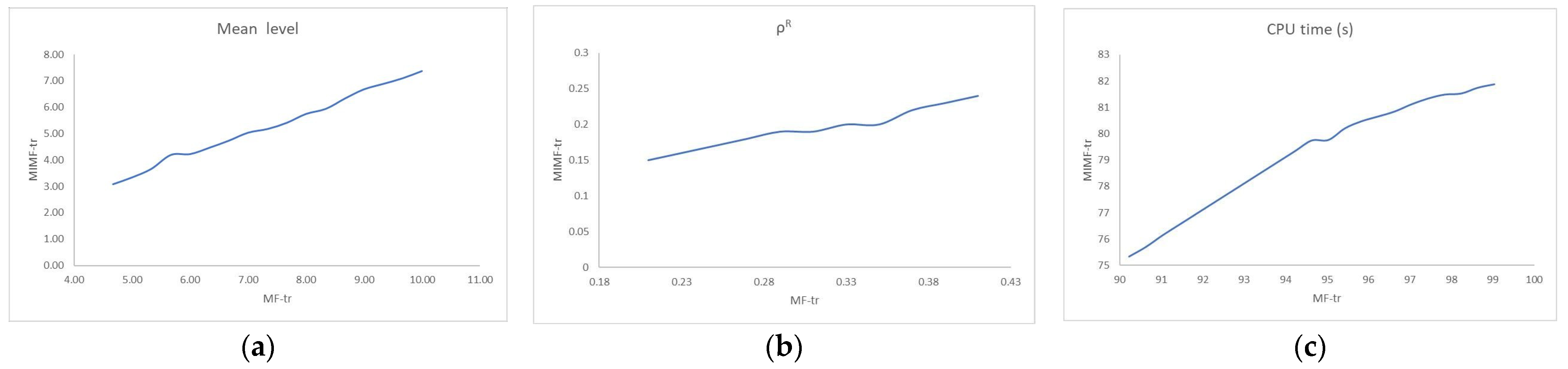
The graphs in
Figure 7a–c show the trend of the mean level, final compression rate, and CPU time obtained, respectively, by executing MIMF-tr with respect to MF-tr for all the satellite images in the dataset. The measurements of the three parameters obtained by executing MIMF-tr are averages obtained by executing MIMF-tr and decomposing the source image into 6, 10, 20, and 30 tiles, respectively.
These results show that for all images, MIMF-tr has better performance than MF-tr, both in terms of the number of levels required for compression and final compression rate and CPU time, regardless of the number of tiles used in MIMF-tr.
Furthermore, the three trends in
Figure 7a–c show that these performances increase as the complexity of the image increases, i.e., the higher the number of levels required for compression, the higher the increase in the final compression rate and CPU time.
5. Conclusions
In this research, a variation of the Multilevel Fuzzy Transform image compression algorithm is proposed to optimize the compression of massive images. The image is decomposed into tiles; each tile is compressed separately by running MF-tr and the compressed tiles are subsequently merged to reconstruct the compressed image.
Our algorithm was tested on an extended sample of large satellite color images. The comparative results showed that, regardless of the number of tiles used, our method performed better than MF-tr both in terms of the number of levels required for compression, as well as the final compression rate and CPU time. Performance is better the more complex the image is, i.e., the greater the number of layers necessary to compress it.
These results highlight, in particular, two significant aspects:
- -
MIMF-tr is better suited than MF-tr for the compression of massive images; the strategy employed by the algorithm of partitioning the image into tiles and separating the compression of single tiles allow for the optimization of processing times and memory consumption;
- -
MIMF-tr provides better performance than MF-tr, reducing the CPU time by more than 20% and providing higher image compression than MF-tr, while ensuring the same reconstructed image quality.
In the future, we intend to carry out further comparative tests on a larger sample of massive images, to verify the performance and robustness of M-ftr in the presence of various types of noise in the image.


