Development of Integrated Linear Programming Fuzzy-Rough MCDM Model for Production Optimization

Abstract

One of the most common tools for achieving optimization and adequate production process management is linear programming (LP) in various forms. However, there are specific cases of the application of linear programming when production optimization implies several potential solutions instead of one. Exactly such a problem is solved in this paper, which integrates linear programming and a Multi-Criteria Decision-Making (MCDM) model. First, linear programming was applied to optimize production and several potential solutions lying on the line segment AB were obtained. A list of criteria was created and evaluated using the Improved Fuzzy Stepwise Weight Assessment Ratio Analysis (IMF SWARA). To obtain the final solution, a novel Rough compromise ranking of alternatives from distance to ideal solution (R-CRADIS) method was developed and verified through comparative analysis. The results show that the integration of linear programming and a Fuzzy-Rough MCDM model can be an exceptional solution for solving specific optimization problems.

1. Introduction

Today, linear programming is one of the most effective mathematical tools for solving economic problems, certainly with the support of computer systems. Along with the development of computer systems, there has been an intensified application of linear programming and other related functions to solve specific economic problems. By applying linear programming, greater efficiency is achieved, and production costs can be significantly reduced, as indicated in [1] in which the authors applied the Mixed-Integer Linear Programming model. This is also confirmed by the authors Chandrawat et al. [2] applying fuzzy linear programming to optimize production costs because, in order to optimize these processes, we must make changes that are allow managers to be well informed [3]. However, taking into account that market conditions change very quickly and that there is uncertainty in every segment of the economic system, integrated models are most frequently applied to optimize various problems, as is the case in this paper, in which we presented a novel Rough CRADIS model in integration with the IMF SWARA method and linear programming. The application of linear programming and multi-criteria models is not rare [4,5,6,7]. Cheng et al. [8] created an integration model of multi-criteria decision analysis (MCDA) and inexact mixed integer linear programming (IMILP) to support the selection of an optimal landfill location and waste-flow-allocation pattern so that the total system cost can be minimized. This model includes qualitative and quantitative indicators, which is an advantage considering that the disadvantage of various multi-objective programming models is that they are basically mathematical and often ignore qualitative and subjective factors [8]. The paper [9] uses an integrated fuzzy multi-criteria model and a multi-objective programming approach for supplier selection and order allocation in a green supply chain. First, the fuzzy analytic hierarchy process and fuzzy TOPSIS were applied in order to analyze the significance of criteria and determine the best green suppliers. Then, multi-objective linear programming was used to consider and formulate various constraints such as quality control, capacity and other objectives. The objective of the mathematical model is simultaneously to maximize the total value of purchasing and to minimize the total cost of purchasing. The subject of research in the paper [10] refers to an integrated approach of multi-attribute utility theory (MAUT) and linear programming (LP) for evaluating and selecting the best suppliers and defining optimal order quantities among the selected ones to maximize total utility.

The following can be identified as special contributions of this paper:

(1) Formation of a novel integrated model consisting of linear programming, IMF SWARA method and Rough CRADIS approach.

(2) Extending the CRADIS approach with Rough Numbers (R-CRADIS) and presenting it for the first time in the literature, which is an enrichment of the entire field that treats multi-criteria problems.

(3) Solving the special case of linear programming obtaining multiple optimal solutions and integration with a MCDM model in order to achieve the desired optimum.

(4) Carrying out a sensitivity analysis based on which decision-makers can make decisions in real time, by looking at the real needs of the company and market requirements at any moment, and by considering the simulated values of criteria and obtaining new optimal solutions.

Motivation and objectives of the paper can be manifested through the following. When applying LP for the optimization and management of production processes in this special case, several potential solutions are obtained instead of one which is usually the case. In order to determine one solution that is optimal under the given circumstances and taking into account various factors, integration with a novel MCDM model was carried out. Moreover, the aim is to develop a model ensuring managers use real-time decision-making.

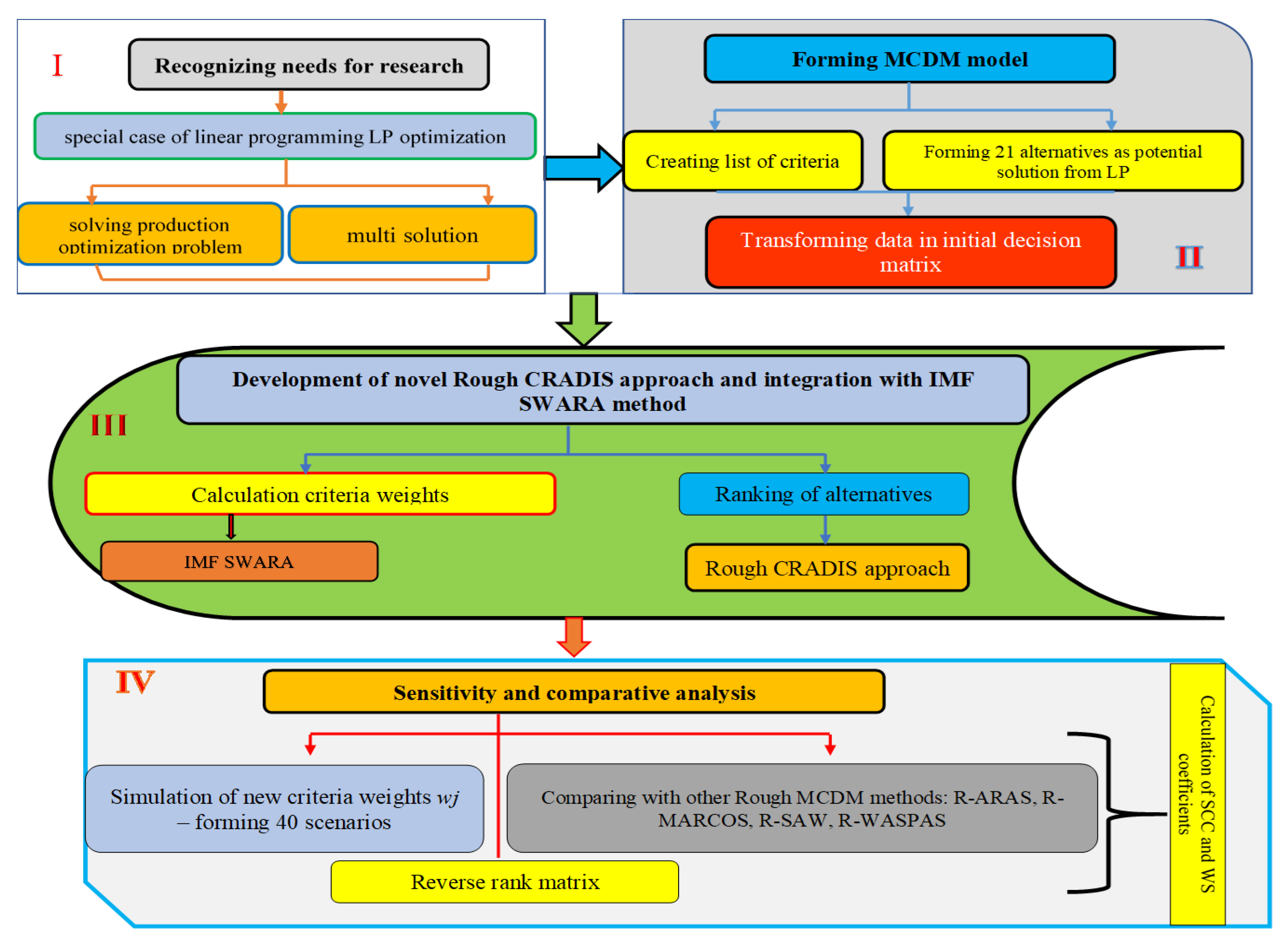
The rest of the paper consists of the following sections. In Section 2, materials and methods are given. The overall flow of the research is presented graphically and the steps of the developed method and applied methods are explained. The development of a novel Rough CRADIS approach is presented in detail. Section 3 introduces the optimization of production with the aim of maximizing profit. A special case of linear programming and its integration with a fuzzy-rough MCDM model is given. Section 4 is also of great importance because it presents the verification of the proposed model through sensitivity analysis, comparative analysis and calculation of statistical SCC and WS coefficients to determine the correlation of the ranks obtained. Finally, Section 5 provides concluding considerations with guidelines for future actions.

2. Materials and Methods

2.1. Methodology Steps

Figure 1 presents the overall methodology of this paper, which is divided into four different phases (I, II, III and IV). The first phase represents the expressed need for solving special problems by LP optimization. Additionally, in this phase, solving the problem of optimizing the production plan is presented with the aim of determining the maximum profit.

When applying LP for the optimization and management of production processes in this special case, several potential solutions are obtained instead of one which is usually the case. In order to determine one solution that is optimal under the given circumstances and taking into account various factors, the integration with a novel MCDM model was carried out. This represents the second phase of the research. First, four criteria were defined: capacity utilization of the first group of machines M (C1), capacity utilization of the second group of machines N (C2), supplying the market with articles of group A (C3) supplying the market with articles of group B (C4). Alternatives represent all potential solutions for x1 = 2000–2500, and for x2 = 1000–2000. A total of 21 potential solutions were created, and then the data were transformed into an initial decision matrix. The third phase involves the development of the novel Rough CRADIS approach (in which computation was made in Microsoft Excel), which represents a contribution from the methodological aspect. The developed approach is used to evaluate potential solutions, while the IMF SWARA method is used to calculate the weights of criteria. The fourth phase is determining the verification of the proposed model through several steps. Using sensitivity analysis and the formation of 40 scenarios, it is possible for decision-makers to determine the optimal solution in real time, which is also one of the contributions of this research both from the methodological and professional aspect. Then the obtained results were compared with four other Rough MCDM methods: Rough WASPAS [11], Rough SAW [12], Rough ARAS [13] and Rough MARCOS [14]. An additional test of the rank stability of potential solutions was also performed by creating 20 new scenarios in which the worst alternative was removed, and the entire procedure was repeated. Finally, statistical correlation tests were calculated for both sensitivity analysis and comparative analysis. Thus, SCC [15] and WS coefficients were calculated [16].

2.2. Linear Programming

The general task of LP: find a non-negative solution

$$X=\left(x_1,x_2,\dots ,x_n\right),(x_i\ge 0,i=1,2,\dots ,n)$$

(1)

of the systems of linear inequalities or equations with constraints:

$$\begin{array}{l}{a}_{11}{x}_1+a_{12}{x}_2+\dots +a_{1n}{x}_n\left\{\underset{\le }{\overset{\ge }{=}}\right\}{b}_1\\ a_{21}{x}_1+a_{22}{x}_2+\dots +a_{2n}{x}_n\left\{\underset{\le }{\overset{\ge }{=}}\right\}{b}_2\\ ⋮\\ a_{m1}{x}_1+a_{m2}{x}_2+\dots +a_{mn}{x}_n\left\{\underset{\le }{\overset{\ge }{=}}\right\}{b}_m\end{array}$$

(2)

so that the linear objective function reaches an extremum, i.e., a minimum or maximum value.

$$F=F\left(x_1,x_2,\dots ,x_n\right)=c_1{x}_1+c_2{x}_2+\dots +c_n{x}_n$$

(3)

The constraints in the LP problem form a domain of admissible solutions, which contains a set of solutions $\overline{C}$. Each point in $\overline{C}$ is a candidate for a solution in the LP problem and is denoted as an admissible solution. A set $\overline{C}$ represents a set of admissible solutions. Among all points in the set $\overline{C}$, the point(s) that optimize(s) the objective function of the LP problem is called the optimal solution of the LP problem.

2.3. IMF SWARA Method

The IMF SWARA method has been created by Vrtagić et al. [17] and consists of the following steps [14,18]:

Step 1: Sorting criteria in descending order based on their expected significance.

Step 2: Relatively smaller significance of each criterion (criterion Cj) is determined in relation to the previous one (Cj − 1), and this is repeated for each subsequent criterion. The comparative significance of the average value is denoted by $\overline{{\wp }_j}$. Linguistics and the TFN scale for assessment of criteria is shown in

Table 1. Linguistics and the TFN scale.

Linguistic Variable	Abbreviation	TFN Scale
Absolutely less significant	ALS	1	1	1
Dominantly less significant	DLS	1/2	2/3	1
Much less significant	MLS	2/5	1/2	2/3
Really less significant	RLS	1/3	2/5	1/2
Less significant	LS	2/7	1/3	2/5
Moderately less significant	MDLS	1/4	2/7	1/3
Weakly less significant	WLS	2/9	1/4	2/7
Equally significant	ES	0	0	0

.

Step 3: Determining the fuzzy coefficient $\overline{{\Im }_j}$ from Equation (4):

$$\overline{{\Im }_j}=\{\begin{array}{l}\overline{1}\hspace{1em}\hspace{1em}\hspace{1em}\hspace{1em}j=1\\ \overline{{\wp }_j}\oplus \overline{1}\hspace{1em}\hspace{1em}j>1\end{array}$$

(4)

The comparative significance of the average value—$\overline{{\wp }_j}$ can then be found.

Step 4: Determining the calculated weights $\overline{{\aleph }_j}$ from Equation (5):

$$\overline{{\aleph }_j}=\{\begin{array}{l}\overline{1}\hspace{1em}\hspace{1em}\hspace{1em}j=1\\ \frac{\overline{{\aleph }_{j-1}}}{\overline{{\Im }_j}}\hspace{1em}\hspace{1em}j>1\end{array}$$

(5)

$\overline{{\Im }_j}$ is the fuzzy coefficient from the previous step.

Step 5: Calculation of the fuzzy weight coefficients, from Equation (6):

$$\overline{w_j}=\frac{\overline{{\aleph }_j}}{{\displaystyle \sum _{j=1}^n\overline{{\aleph }_j}}}$$

(6)

where $\overline{w_j}$ represents the fuzzy relative weight of the criteria j, and n represents the number of criteria.

2.4. Development of a Novel Rough CRADIS Approach

In this section of the paper, the CRADIS approach [19,20,21] was extended with Rough numbers. The developed Rough CRADIS approach is described through the following steps and equations.

Step 1. The first step includes the formation of an initial Rough decision matrix consisting of n criteria and m alternatives as shown in Equation (7),

$$\xi =\left[\begin{array}{c}\left[{\xi }_{11}^L,{\xi }_{11}^U\right]\\ \left[{\xi }_{21}^L,{\xi }_{21}^U\right]\\ ⋮\\ \left[{\xi }_{m1}^L,{\xi }_{m1}^U\right]\end{array}\begin{array}{c}\left[{\xi }_{12}^L,{\xi }_{12}^U\right]\\ \left[{\xi }_{22}^L,{\xi }_{22}^U\right]\\ ⋮\\ \left[{\xi }_{m2}^L,{\xi }_{m2}^U\right]\end{array}\begin{array}{c}\cdots \\ \cdots \\ \ddots \\ \cdots \end{array}\begin{array}{c}\left[{\xi }_{1n}^L,{\xi }_{1n}^U\right]\\ \left[{\xi }_{2n}^L,{\xi }_{2n}^U\right]\\ ⋮\\ \left[{\xi }_{mn}^L,{\xi }_{mn}^U\right]\end{array}\right]$$

(7)

where ${\xi }_{ij}$ denotes the performance of alternative m in relation to criterion n.

Step 2. Determination of a Rough normalized decision matrix (8) using Equations (9) and (10):

$$\varsigma =\left[\begin{array}{c}\left[{\varsigma }_{11}^L,{\varsigma }_{11}^U\right]\\ \left[{\varsigma }_{21}^L,{\varsigma }_{21}^U\right]\\ ⋮\\ \left[{\varsigma }_{m1}^L,{\varsigma }_{m1}^U\right]\end{array}\begin{array}{c}\left[{\varsigma }_{12}^L,{\varsigma }_{12}^U\right]\\ \left[{\varsigma }_{22}^L,{\varsigma }_{22}^U\right]\\ ⋮\\ \left[{\varsigma }_{m2}^L,{\varsigma }_{m2}^U\right]\end{array}\begin{array}{c}\cdots \\ \cdots \\ \ddots \\ \cdots \end{array}\begin{array}{c}\left[{\varsigma }_{1n}^L,{\varsigma }_{1n}^U\right]\\ \left[{\varsigma }_{2n}^L,{\varsigma }_{2n}^U\right]\\ ⋮\\ \left[{\varsigma }_{mn}^L,{\varsigma }_{mn}^U\right]\end{array}\right]$$

(8)

$${\varsigma }_{ij}=\frac{{\xi }_{ij}}{\max {\xi }_{ij}}=\left[\frac{{\xi }_{ij}^L}{\max {\xi }_{ij}^U},\frac{{\xi }_{ij}^U}{\max {\xi }_{ij}^L}\right],\hspace{1em}j\in B$$

(9)

where B marks a set of benefit criteria, and

$${\varsigma }_{ij}=\frac{\min {\xi }_{ij}}{{\xi }_{ij}}=\left[\frac{\min {\xi }_{ij}^L}{{\xi }_{ij}^U},\frac{\min {\xi }_{ij}^U}{{\xi }_{ij}^L}\right],\hspace{1em}j\in C$$

(10)

where C marks a set of cost criteria.

Step 3. Calculation of the weighted normalized Rough matrix (11) using Equation (12):

$$\upsilon =\left[\begin{array}{c}\left[{\upsilon }_{11}^L,{\upsilon }_{11}^U\right]\\ \left[{\upsilon }_{21}^L,{\upsilon }_{21}^U\right]\\ ⋮\\ \left[{\upsilon }_{m1}^L,{\upsilon }_{m1}^U\right]\end{array}\begin{array}{c}\left[{\upsilon }_{12}^L,{\upsilon }_{12}^U\right]\\ \left[{\upsilon }_{22}^L,{\upsilon }_{22}^U\right]\\ ⋮\\ \left[{\upsilon }_{m2}^L,{\upsilon }_{m2}^U\right]\end{array}\begin{array}{c}\cdots \\ \cdots \\ \ddots \\ \cdots \end{array}\begin{array}{c}\left[{\upsilon }_{1n}^L,{\upsilon }_{1n}^U\right]\\ \left[{\upsilon }_{2n}^L,{\upsilon }_{2n}^U\right]\\ ⋮\\ \left[{\upsilon }_{mn}^L,{\upsilon }_{mn}^U\right]\end{array}\right]$$

(11)

$${\upsilon }_{ij}={\varsigma }_{ij}\otimes w_j=\left[{\varsigma }_{ij}^L\otimes w_j^L,{\varsigma }_{ij}^U\otimes w_j^U\right]$$

(12)

Step 4. Calculation of an ideal ${\tau }_{id}$ (the largest value of ${\upsilon }_{ij}$) and anti-ideal solution ${\tau }_{aid}$ (the smallest value ${\upsilon }_{ij}$).

$${\tau }_{id}={\left[{\tau }_{id}^L,{\tau }_{id}^U\right]}_{1\times n}=\max {\upsilon }_{ij}$$

(13)

$${\tau }_{aid}={\left[{\tau }_{aid}^L,{\tau }_{aid}^U\right]}_{1\times n}=\min {\upsilon }_{ij}$$

(14)

Step 5. Determination of deviations from ideal and anti-ideal solutions, Equations (15) and (16).

$${\delta }_{ij}^{+}={\left[{\delta }_{ij}^{+L},{\delta }_{ij}^{+U}\right]}_{m\times n}=\max {\tau }_{id}-{\upsilon }_{ij}=\left[\max {\tau }_{ij}^L-{\upsilon }_{ij}^U,\max {\tau }_{ij}^U-{\upsilon }_{ij}^L\right]$$

(15)

$${\delta }_{ij}^{-}={\left[{\delta }_{ij}^{-L},{\delta }_{ij}^{-U}\right]}_{m\times n}={\upsilon }_{ij}-\min {\tau }_{aid}=\left[{\upsilon }_{ij}^L-\min {\tau }_{ij}^U,{\upsilon }_{ij}^U-\min {\tau }_{ij}^L\right]$$

(16)

Step 6. Calculation of the degree of deviation of each alternative from ideal and anti-ideal solutions.

$${\Re }_i^{+}={\left[{\Re }_i^{+L},{\Re }_i^{+U}\right]}_{1\times m}={\displaystyle \sum _{j=1}^n{\delta }_{ij}^{+}}$$

(17)

$${\Re }_i^{-}={\left[{\Re }_i^{-L},{\Re }_i^{-U}\right]}_{1\times m}={\displaystyle \sum _{j=1}^n{\delta }_{ij}^{-}}$$

(18)

Step 7. Determination of the utility function of each alternative relative to the optimal alternatives.

$$\begin{array}{l}{\hslash }_i^{+}={\left[{\hslash }_i^{+L},{\hslash }_i^{+U}\right]}_{1\times m}=\left[\frac{{\Re }_o^{+}}{{\Re }_i^{+}}\right]=\left[\frac{{\Re }_o^{+L}}{{\Re }_i^{+U}},\frac{{\Re }_o^{+U}}{{\Re }_i^{+L}}\right]\\ {\Re }_o^{+}={\displaystyle \sum _{j=1}^n\left(\min \left({\delta }_{ij}^{+}\right)\right)}\end{array}$$

(19)

$$\begin{array}{l}{\hslash }_i^{-}={\left[{\hslash }_i^{-L},{\hslash }_i^{-U}\right]}_{1\times m}=\left[\frac{{\Re }_o^{-}}{{\Re }_i^{-}}\right]=\left[\frac{{\Re }_o^{-L}}{{\Re }_i^{-U}},\frac{{\Re }_o^{-U}}{{\Re }_i^{-L}}\right]\\ {\Re }_o^{-}={\displaystyle \sum _{j=1}^n\left(\min \left({\delta }_{ij}^{-}\right)\right)}\end{array}$$

(20)

Step 8. Sorting alternatives by calculating the average utility function using Equation (21). The best alternative is the one with the highest value.

$${\chi }_i={\left[{\chi }_i^{-L},{\chi }_i^{-U}\right]}_{1\times m}=\left[\frac{{\hslash }_i^{+}+{\hslash }_i^{-}}{2}\right]=\left[\frac{{\hslash }_i^{+L}+{\hslash }_i^{-L}}{2},\frac{{\hslash }_i^{+U}+{\hslash }_i^{-U}}{2}\right]$$

(21)

3. Integration of Linear Programming and a Fuzzy-Rough MCDM Model for Production Optimization

3.1. Special Case of Linear Programming Optimization

The company produces two articles, A and B, on two groups of machines, M and N. In the period considered, the first group of machines has a capacity of 6000 working hours, and the second group has a capacity of 3000 working hours. The processing time of a unit of article A is 1.5 working hours on the first group of machines, and 1 working hour on the second group of machines. The processing time of a unit of article B is 1.5 working hours on the first group of machines, and 0.5 working hour on the second group of machines. For the production realization, the company has enough raw materials and labor, but it can only put 2500 units of article A and 3000 units of article B on the market. By selling, the company makes a profit of 2000 monetary units per unit of article A and 1000 monetary units per unit of article B. It is necessary to determine the optimal production plan in order to achieve the maximum profit for the company.

First of all, it is necessary to set up a mathematical model in accordance with Equations (1)–(3). Constraints of the model according to the parameters of the study are as follows:

$$\begin{array}{l}\frac{3}{2}{x}_1+\frac{3}{2}{x}_2\le 6000\\ x_1+\frac{1}{2}{x}_2\le 3000\\ \hspace{1em}\hspace{1em}\hspace{1em}{x}_1\le 2500\\ \hspace{1em}\hspace{1em}\hspace{1em}{x}_2\le 3000\\ \hspace{1em}\hspace{1em}{x}_1,x_2\ge 0\end{array}$$

while the objective function of maximizing the company’s profit is presented as follows:

$$F_{\max }=2000x_1+1000x_2$$

By applying the simplex method of linear programming (Simplex Method calculator), the values of the objective function presented in

Table 2. Value of function F.

x1	X2	S1	S2	S3	S4	Const.
0	0	1	−3	3/2	0	750
0	1	0	2	−2	0	1000
1	0	0	0	1	0	2500
0	0	0	−2	2	1	2000
0	0	0	−2000	0	0	F − 6000000
0	0	2/3	−2	1	0	500
0	1	0	2	−2	0	1000
1	0	0	0	1	0	2500
0	0	0	−2	2	1	2000
0	0	0	−2000	0	0	F − 6000000
0	0	2/3	−2	1	0	500
0	1	4/3	−2	0	0	2000
1	0	−2/3	2	0	0	2000
0	0	−4/3	2	0	1	1000
0	0	0	−2000	0	0	F − 6000000

are obtained.

Non-basic variables are zero. The value of the basic variables can be taken into account. The function F contains only non-basic variables. Thus, the value of the function F for the basis can be kept in mind.

$$\begin{array}{l}{S}_1=0,\hspace{1em}{S}_2=0,\hspace{1em}{S}_3=500,\hspace{1em}{S}_4=1000\\ x_1=2000,\hspace{1em}{x}_2=2000\\ F-6000000=0\Rightarrow F=6000000\end{array}$$

(22)

From a geometric point of view, both solutions are points of space, i.e., they form a line segment. Any point (any solution) on this segment will also be a solution.

Finally, the result of linear programming is presented by the following function:

$$\begin{array}{l}{x}_1=2500t+2000\left(1-t\right)\\ x_2=1000t+2000\left(1-t\right)\\ 0\le t\le 1\\ F_{\max }=6000000\end{array}$$

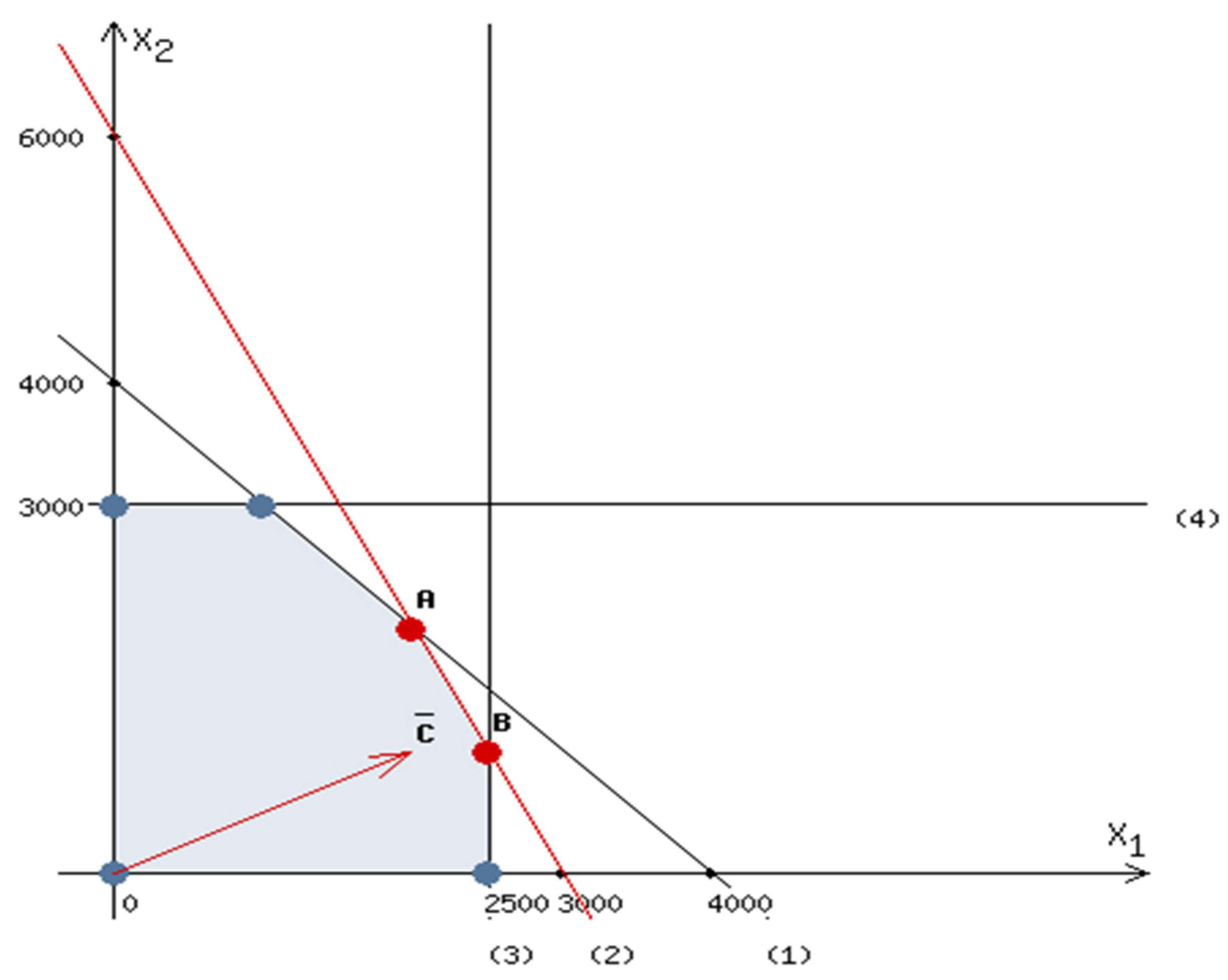
The optimal solution is represented by the extreme points, A and B, of the convex set C (Figure 2). In other words, the optimal solution is represented by every point of the line segment AB.

The maximum value of the objective function is as follows:

$$F_{\max }(X)=F(A)=2000(2000)+1000(2000)=6000000$$

(23)

i.e.,

$$F_{\max }(X)=F(B)=2000(2500)+1000(1000)=6000000$$

(24)

We will obtain the same value of the criterion function if we include the coordinates of any point on the line segment AB, which represents a large number of admissible optimal solutions. The optimal value of the objective function is unique because it is six million regardless of how many products A and how many products B will be produced, but there are infinitely many admissible solutions that provide this function value.

The multiplicity of the optimal solution gives greater opportunities to the decision-maker, and this is where MCDM methods come into focus. The decision-maker chooses an optimal solution that best fits these conditions, e.g., if the extreme point B is taken as the optimal solution, then the capacity of the second group of machines will be fully utilized, while the first group of machines will have an unused capacity of 750 working hours. The market will be fully supplied by the first article, and it will lack 2000 units of article B. Which solution the decision-maker will choose depends on whether it is more important for him to use the capacity of the machines or to supply the market with articles individually. It is through the further development of the multi-criteria Fuzzy-Rough MCDM model that the optimal solution is reached depending on the current needs of the company, and it is defined through determining the significance of the criteria and extensive sensitivity analysis.

3.2. Formation of MCDM Model—Defining Criteria and Alternatives

Since we have as a solution many points that represent the optimal solution, a multi-criteria model can be applied further. Four criteria are defined: capacity utilization of the first group of machines M (C1), capacity utilization of the second group of machines N (C2), supplying the market with articles of group A (C3) and supplying the market with articles of group B (C4). A total of 21 alternatives were defined in accordance with the value t = 0–1 with an interval of 0.05 (

Table 3. Defining alternatives depending on the value t.

	t	x1	x2
A1	1	2500	1000
A2	0.095	2475	1050
A3	0.090	2450	1100
A4	0.085	2425	1150
A5	0.080	2400	1200
A6	0.075	2375	1250
A7	0.070	2350	1300
A8	0.065	2325	1350
A9	0.060	2300	1400
A10	0.055	2275	1450
A11	0.050	2250	1500
A12	0.045	2225	1550
A13	0.040	2200	1600
A14	0.035	2175	1650
A15	0.030	2150	1700
A16	0.025	2125	1750
A17	0.020	2100	1800
A18	0.015	2075	1850
A19	0.010	2050	1900
A20	0.05	2025	1950
A21	0	2000	2000

):

3.3. Determining the Significance of Criteria Using the IMF SWARA Method

In this section of the paper, the calculation of weight values of the criteria was carried out using the IMF SWARA method. It is not group decision-making because previously it was a specific optimization problem using linear programming, after which the decision-maker takes into account the current state and needs of the company and evaluates the criteria as shown in

Table 4. Weight values of the criteria calculated with the IMF SWARA method.

	$\overline{{\mathit{\wp }}_{\mathit{j}}}$	$\overline{{\mathit{\Im }}_{\mathit{j}}}$			$\overline{{\mathit{\aleph }}_{\mathit{j}}}$			$\overline{{\mathit{w}}_{\mathit{j}}}$
C3		1.000	1.000	1.000	1.000	1.000	1.000	0.287	0.291	0.296
C4	ES	1.000	1.000	1.000	1.000	1.000	1.000	0.287	0.291	0.296
C1	WLS	1.222	1.250	1.286	0.778	0.800	0.818	0.223	0.233	0.242
C2	WLS	1.222	1.250	1.286	0.605	0.640	0.669	0.173	0.186	0.198
				SUM	3.383	3.440	3.488

.

First, the linguistic values of the criterion comparison $\overline{{\wp }_j}$ are defined, and the values $\overline{{\Im }_j}$ for j > 1 are obtained by adding TFN (1,1,1). The values $\overline{{\aleph }_j}$ for j > 1 are obtained as follows: $\overline{{\aleph }_1}=\frac{\overline{{\aleph }_{1-1}}}{\overline{{\Im }_1}}=\frac{\overline{{\aleph }_4}}{\overline{{\Im }_1}}=\left(\frac{1}{1.286},\frac{1}{1.250},\frac{1}{1.222}\right)=\left(0.778,0.800,0.818\right)$. The final fuzzy criterion weights are obtained as follows:

$$\overline{w_1}=\frac{\overline{{\aleph }_1}}{{\displaystyle \sum _{j=1}^n\overline{{\aleph }_j}}}=\left(\frac{1}{3.488},\frac{1}{3.440},\frac{1}{3.383}\right)=\left(0.287,0.291,0.296\right).$$

The results show that the decision-maker views the significance of the criteria quite equally, so did not decide to assign much greater significance to any one criterion than to the others. Even the highest-ranked criterion is not much more significant compared to the least significant one.

3.4. Determining the Optimal Solution Using the Rough CRADIS Approach

In Section 3.2, alternative values of t and values of x₁ and x₂ are defined, by including the values of x₁ and x₂ in each constraint, as e.g., for A1:

$$\begin{array}{l}\frac{3}{2}\times 2500+\frac{3}{2}\times 1000=5250\le 6000\hspace{1em}\left(750\right)\\ \hspace{1em} 2500+\frac{1}{2}\times 1000=3000\hspace{1em}\left(0\right)\\ \hspace{1em}\hspace{1em}\hspace{1em}\hspace{1em}\hspace{1em}\hspace{1em}2500=2500\hspace{1em}\left(0\right)\\ \hspace{1em}\hspace{1em}\hspace{1em}\hspace{1em}\hspace{1em}\hspace{1em}1000\le 3000\hspace{1em}\left(2000\right)\end{array}$$

For A2:

$$\begin{array}{l}\frac{3}{2}\times 2475+\frac{3}{2}\times 1050=5287.5\le 6000\hspace{1em}\left(712.5\right)\\ \hspace{1em} 2475+\frac{1}{2}\times 1050=3000\hspace{1em}\left(0\right)\\ \hspace{1em}\hspace{1em}\hspace{1em}\hspace{1em}\hspace{1em}\hspace{1em}2475\le 2500\hspace{1em}\left(25\right)\\ \hspace{1em}\hspace{1em}\hspace{1em}\hspace{1em}\hspace{1em}\hspace{1em}1050\le 3000\hspace{1em}\left(1950\right)\end{array}$$

For A21:

$$\begin{array}{l}\frac{3}{2}\times 2000+\frac{3}{2}\times 2000=6000\hspace{1em}\left(0\right)\\ \hspace{1em} 2000+\frac{1}{2}\times 2000=3000\hspace{1em}\left(0\right)\\ \hspace{1em}\hspace{1em}\hspace{1em}\hspace{1em}\hspace{1em}\hspace{1em}2000\le 2500\hspace{1em}\left(500\right)\\ \hspace{1em}\hspace{1em}\hspace{1em}\hspace{1em}\hspace{1em}\hspace{1em}2000\le 3000\hspace{1em}\left(1000\right)\end{array}$$

In this way, the complete initial decision matrix is obtained as shown in

Table 5. Initial decision matrix.

	C1		C2		C3		C4
A1	750.00	750.00	1	1	1	1	2000	2000
A2	712.50	712.50	1	1	25	25	1950	1950
A3	675.00	675.00	1	1	50	50	1900	1900
A4	637.50	637.50	1	1	75	75	1850	1850
A5	600.00	600.00	1	1	100	100	1800	1800
A6	562.50	562.50	1	1	125	125	1750	1750
A7	525.00	525.00	1	1	150	150	1700	1700
A8	487.50	487.50	1	1	175	175	1650	1650
A9	450.00	450.00	1	1	200	200	1600	1600
A10	412.50	412.50	1	1	225	225	1550	1550
A11	375.00	375.00	1	1	250	250	1500	1500
A12	337.50	337.50	1	1	275	275	1450	1450
A13	300.00	300.00	1	1	300	300	1400	1400
A14	262.50	262.50	1	1	325	325	1350	1350
A15	225.00	225.00	1	1	350	350	1300	1300
A16	187.50	187.50	1	1	375	375	1250	1250
A17	150.00	150.00	1	1	400	400	1200	1200
A18	112.50	112.50	1	1	425	425	1150	1150
A19	75.00	75.00	1	1	450	450	1100	1100
A20	37.50	37.50	1	1	475	475	1050	1050
A21	1.00	1.00	1	1	500	500	1000	1000

, which essentially represents the difference in satisfying the set restrictions for each criterion separately. For example, for A1, the values of x₁ and x₂ are 2500 and 1000, respectively, and the utilization of the first group of machines M is not complete, but there are still 750 h available, while the second group of machines N is fully utilized. When it comes to meeting the requirements of the market with product A, it is fully satisfied, while there is a shortage of 2000 products B according to these parameters. The initial decision-making matrix represents equal low and upper numbers because it represents the difference in satisfying the set restrictions for each criterion separately which is essential for managers while having no influence on the application of the rough model.

By Equations (8)–(21), the final results of applying the new Rough CRADIS approach are obtained, which is shown in

Table 6. Results of applying the Rough CRADIS approach.

	${\mathit{\Re }}_{\mathit{i}}^{+}$	${\mathit{\Re }}_{\mathit{i}}^{-}$	${\mathit{\Re }}_{\mathit{o}}^{+}$	${\mathit{\Re }}_{\mathit{o}}^{-}$	${\mathit{\hslash }}_{\mathit{i}}^{+}$	${\mathit{\hslash }}_{\mathit{i}}^{-}$	${\mathit{\chi }}_{\mathit{i}}$	Rank
A1	0.9465	0.6685	0.6165	0.9985	0.6514	0.669542	0.660	1
A2	1.3343	0.2807			0.4621	0.281146	0.372	3
A3	1.3422	0.2729			0.4594	0.273271	0.366	7
A4	1.3446	0.2704			0.4585	0.270808	0.365	11
A5	1.3457	0.2693			0.4581	0.269709	0.364	14
A6	1.3463	0.2688			0.4580	0.269167	0.364	17
A7	1.3465	0.2685			0.4579	0.268913	0.363	19
A8	1.3466	0.2684			0.4578	0.268834	0.363	21
A9	1.3466	0.2685			0.4579	0.268876	0.363	20
A10	1.3464	0.2686			0.4579	0.269011	0.363	18
A11	1.3462	0.2688			0.4580	0.269222	0.364	16
A12	1.3459	0.2691			0.4581	0.269506	0.364	15
A13	1.3456	0.2695			0.4582	0.269862	0.364	13
A14	1.3451	0.2699			0.4583	0.270297	0.364	12
A15	1.3446	0.2704			0.4585	0.270829	0.365	10
A16	1.3439	0.2711			0.4587	0.271487	0.365	9
A17	1.3431	0.2719			0.4590	0.272337	0.366	8
A18	1.3419	0.2731			0.4594	0.273524	0.366	6
A19	1.3400	0.2751			0.4601	0.275485	0.368	5
A20	1.3351	0.2800			0.4618	0.280383	0.371	4
A21	1.0199	0.5951			0.6045	0.596012	0.600	2

.

After applying the Rough CRADIS model, the optimal solution is alternative A1, while the alternative A21 represents the second best solution under the given conditions and parameters of the model.

4. Verification of the Developed Model and Discussion

4.1. Sensitivity Analysis

The sensitivity analysis has been performed through 40 scenarios that represent new simulated criterion values using Equation (22) [22,23,24]:

$${\overline{W}}_{n\beta }=\left(1-{\overline{W}}_{n\alpha }\right)\frac{{\overline{W}}_{n=\beta }}{\left(1-{\overline{W}}_n\right)}$$

(25)

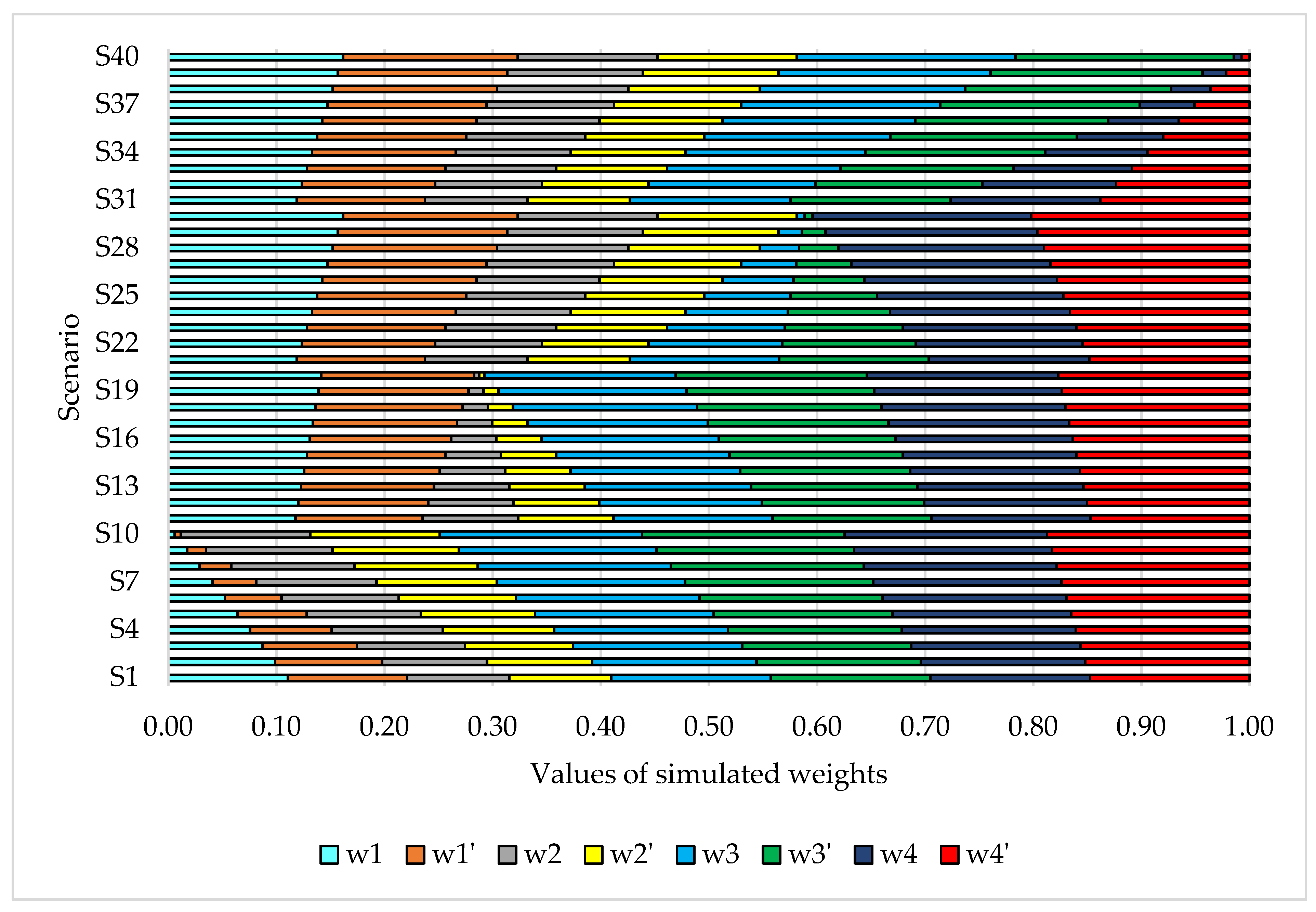
The new criterion values are shown in Figure 3, where the values are simulated as follows: starting from the first scenario in which the value of criterion C1 is reduced by 5% to S10 in which the value of that criterion is reduced by 95%, while the values of criteria C2, C3 and C4 increase proportionally. In the same way, new criterion values are determined in S11–S20 for C2, in S21–S30 for C3 and in S31–S40 for C4.

Figure 4 shows the ranks of all alternatives depending on the simulated weight values of the criteria.

The change in the ranks of alternatives is obvious so, e.g., A1 in S4–S10 is in the first position, which is a consequence of the reduction of C1 criterion by 35–95% while, e.g., in S27–S30, its rank decreases drastically to the 7th, 11th, 14th and 19th position, respectively, which is a consequence of the decrease in the significance of criterion C3 by 65–95%. This kind of sensitivity analysis in this special case of searching for an optimal solution represents an exceptional contribution for the decision-maker because he can fully perceive the real needs and determine which solution is optimal in real time.

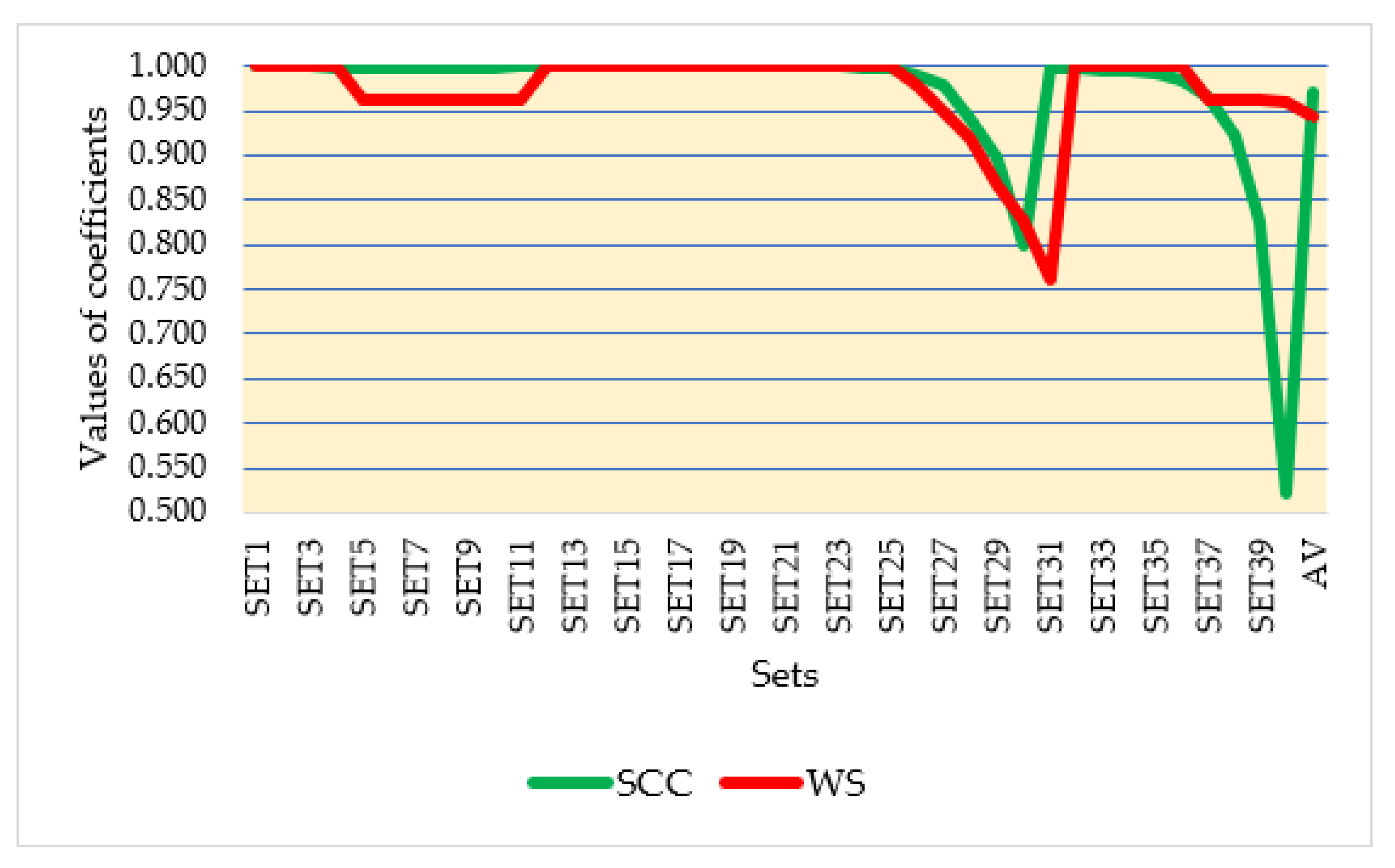
Since there are certain changes in the ranks of potential solutions when reducing the weight values of the criteria, a statistical correlation of the ranks is performed (Figure 5), SCC and WS, which has already been mentioned in the methodology section of the paper. The lowest SCC = 0.521 is in set 40 since A3 drastically increases its position with a total decrease in the value of criterion C4. The lowest WS = 0.762 is in set 31, when the value of the third criterion decreases. Considering the large set of potential solutions (21), the average values of both coefficients show a very high level of rank correlation: SCC = 0.970, WS = 0.944.

4.2. Comparative Analysis

Comparative analysis represents one of the ways of testing the results obtained [25]. As already mentioned, the comparative analysis involves a comparison with four other Rough MCDM methods: Rough WASPAS [11], Rough SAW [12], Rough ARAS [13] and Rough MARCOS [14]. The results of the comparative analysis are shown in Figure 6.

Compared to three Rough MCDM methods, there is no change in the best alternative, while when applying the Rough ARAS method, the two best alternatives exchange places. Moreover, the greatest changes are in the comparison of Rough CRADIS with the Rough ARAS method, where A3 changes its position by several places.

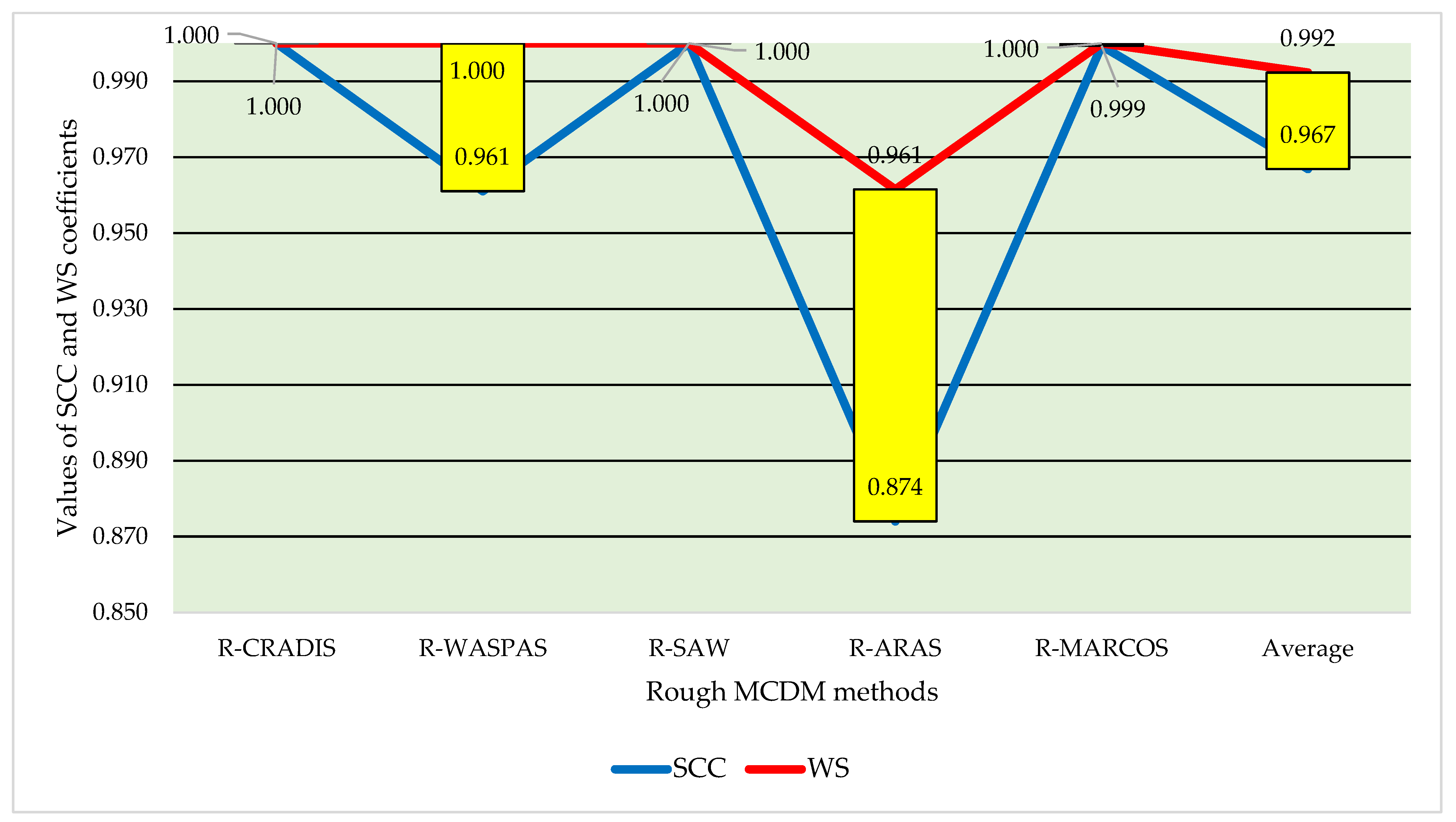
Figure 7 shows the values of SCC and WS coefficients in the comparative analysis.

Rough CRADIS has a full correlation of ranks with Rough SAW, while it has 0.999 with Rough MARCOS, 0.874 with Rough ARAS, and 0.961 with Rough WASPAS when it comes to the SCC coefficient. The situation is similar with the WS coefficient, which has a full correlation with R-WASPAS, R-SAW, R-MARCOS.

4.3. Limitations and Managerial Implications

Limitations of the solution proposed by this research can be traced to linear programming and MCDM methodology. From the aspect of linear programming, the number of variables can represent limitations, while the developed Rough CRADIS model can be applied for group decision-making only, which is the second limitation.

It is very important to note that sensitivity analysis enables real-time decision-making since the decision-maker has at his disposal a set of 40 formed scenarios in which the criteria change their original values. This means that in real time, if it is more important for the company to satisfy the requirements of the market with product B rather than A, it can precisely determine from the obtained results what quantity of product it needs. The same is the case with the use of own resources, which are presented in the paper as criteria.

5. Conclusions

The paper proposes a novel integrated model consisting of a combination of linear programming, fuzzy set theory, rough set theory and a MCDM method. A novel Rough CRADIS approach has been created that can be used for any problem involving multiple criteria. The problem of optimizing production with the aim of maximizing profit, which represents a specific problem of linear programming, has been presented and solved. Based on a numerical example using linear programming, a set of optimal solutions that lie on the line segment AB has been obtained. After that, a total of 21 different solutions were formed, which can represent the optimum depending on the real requirements of the market and the orientation of the company. The IMF SWARA method was applied in order to determine the significance of the criteria considered when making a decision. At the end, a calculation was made using the novel Rough CRADIS approach in order to determine the optimal solution under the given conditions, i.e., how many products should be produced. The results show that the integration of linear programming and a Fuzzy-Rough MCDM model can be an exceptional solution for solving specific optimization problems.

Future research can be reflected through defining a larger number of influential factors and defining an objective function that will minimize costs while maximizing the profit. In addition, the application of fuzzy linear programming with the development of new approaches is highlighted as a useful option.

References

1. Bayá, G.; Canale, E.; Nesmachnow, S.; Robledo, F.; Sartor, P. Production Optimization in a Grain Facility through Mixed-Integer Linear Programming. Appl. Sci. 2022, 12, 8212. [Google Scholar] [CrossRef]
2. Chandrawat, R.K.; Kumar, R.; Garg, B.P.; Dhiman, G.; Kumar, S. An analysis of modeling and optimization production cost through fuzzy linear programming problem with symmetric and right angle triangular fuzzy number. In Proceedings of the Sixth International Conference on Soft Computing for Problem Solving; Springer: Singapore, 2017; pp. 197–211. [Google Scholar]
3. Pop, O.B.; Uifălean, D.C. The Impact of Innovation on the Management of Misapplication of Change in the Production System in the Automotive Industry. Econ. Innov. Econ. Res. J. 2022, 10, 199–210. [Google Scholar]
4. Lazzerini, B.; Pistolesi, F. A linear programming-driven MCDM approach for multi-objective economic dispatch in smart grids. In Proceedings of the 2015 SAI Intelligent Systems Conference (IntelliSys), London, UK, 10–11 November 2015; pp. 475–484. [Google Scholar]
5. Khalilzadeh, M.; Ghasemi, P.; Afrasiabi, A.; Shakeri, H. Hybrid fuzzy MCDM and FMEA integrating with linear programming approach for the health and safety executive risks: A case study. J. Model. Manag. 2021, 16, 1025–1053. [Google Scholar] [CrossRef]
6. Malekpoor, H.; Chalvatzis, K.; Mishra, N.; Mehlawat, M.K.; Zafirakis, D.; Song, M. Integrated grey relational analysis and multi objective grey linear programming for sustainable electricity generation planning. Ann. Oper. Res. 2018, 269, 475–503. [Google Scholar] [CrossRef]
7. Razak, N.H.; Hashim, H.; Yunus, N.A.; Klemeš, J. Integrated linear programming and analytical hierarchy process method for diesel/biodiesel/butanol in reducing diesel emissions. J. Clean. Prod. 2022, 337, 130297. [Google Scholar] [CrossRef]
8. Cheng, S.; Chan, C.W.; Huang, G.H. An integrated multi-criteria decision analysis and inexact mixed integer linear programming approach for solid waste management. Eng. Appl. Artif. Intell. 2003, 16, 543–554. [Google Scholar] [CrossRef]
9. Kannan, D.; Khodaverdi, R.; Olfat, L.; Jafarian, A.; Diabat, A. Integrated fuzzy multi criteria decision making method and multi-objective programming approach for supplier selection and order allocation in a green supply chain. J. Clean. Prod. 2013, 47, 355–367. [Google Scholar] [CrossRef]
10. Sanayei, A.; Mousavi, S.F.; Abdi, M.R.; Mohaghar, A. An integrated group decision-making process for supplier selection and order allocation using multi-attribute utility theory and linear programming. J. Frankl. Inst. 2008, 345, 731–747. [Google Scholar] [CrossRef]
11. Stojić, G.; Stević, Ž.; Antuchevičienė, J.; Pamučar, D.; Vasiljević, M. A novel rough WASPAS approach for supplier selection in a company manufacturing PVC carpentry products. Information 2018, 9, 121. [Google Scholar] [CrossRef]
12. Durmić, E.; Stević, Ž.; Chatterjee, P.; Vasiljević, M.; Tomašević, M. Sustainable supplier selection using combined FUCOM–Rough SAW model. Rep. Mech. Eng. 2020, 1, 34–43. [Google Scholar] [CrossRef]
13. Zavadskas, E.K.; Nunić, Z.; Stjepanović, Ž.; Prentkovskis, O. A novel rough range of value method (R-ROV) for selecting automatically guided vehicles (AGVs). Stud. Inform. Control 2018, 27, 385–394. [Google Scholar] [CrossRef]
14. Vojinović, N.; Sremac, S.; Zlatanović, D. A Novel Integrated Fuzzy-Rough MCDM Model for Evaluation of Companies for Transport of Dangerous Goods. Complexity 2021, 2021, 1–16. [Google Scholar] [CrossRef]
15. Kumar, S.; Maity, S.R.; Patnaik, L. Optimization of Wear Parameters for Duplex-TiAlN Coated MDC-K Tool Steel Using Fuzzy MCDM Techniques. Oper. Res. Eng. Sci. Theory Appl. 2022. [Google Scholar] [CrossRef]
16. Sałabun, W.; Urbaniak, K. A new coefficient of rankings similarity in decision-making problems. In Proceedings of the International Conference on Computational Science, Amsterdam, The Netherlands, 3–5 June 2020; Springer: Cham, Switzerland, 2020; pp. 632–645. [Google Scholar]
17. Vrtagić, S.; Softić, E.; Subotić, M.; Stević, Ž.; Dordevic, M.; Ponjavic, M. Ranking road sections based on MCDM model: New improved fuzzy SWARA (IMF SWARA). Axioms 2021, 10, 92. [Google Scholar] [CrossRef]
18. Zolfani, S.H.; Görçün, Ö.F.; Küçükönder, H. Evaluating logistics villages in Turkey using hybrid improved fuzzy SWARA (IMF SWARA) and fuzzy MABAC techniques. Technol. Econ. Dev. Econ. 2021, 27, 1582–1612. [Google Scholar] [CrossRef]
19. Puška, A.; Božanić, D.; Nedeljković, M.; Janošević, M. Green Supplier Selection in an Uncertain Environment in Agriculture Using a Hybrid MCDM Model: Z-Numbers–Fuzzy LMAW–Fuzzy CRADIS Model. Axioms 2022, 11, 427. [Google Scholar] [CrossRef]
20. Puška, A.; Stević, Ž.; Pamučar, D. Evaluation and selection of healthcare waste incinerators using extended sustainability criteria and multi-criteria analysis methods. Environ. Dev. Sustain. 2022, 24, 11195–11225. [Google Scholar] [CrossRef]
21. Puška, A.; Nedeljković, M.; Prodanović, R.; Vladisavljević, R.; Suzić, R. Market assessment of pear varieties in Serbia using fuzzy CRADIS and CRITIC methods. Agriculture 2022, 12, 139. [Google Scholar] [CrossRef]
22. Božanić, D.; Milić, A.; Tešić, D.; Salabun, W.; Pamučar, D. D numbers–FUCOM–fuzzy RAFSI model for selecting the group of construction machines for enabling mobility. Facta Univ. Ser. Mech. Eng. 2021, 19, 447–471. [Google Scholar] [CrossRef]
23. Mešić, A.; Miškić, S.; Stević, Ž.; Mastilo, Z. Hybrid MCDM solutions for evaluation of the logistics performance index of the Western Balkan countries. Econ.-Innov. Econ. Res. J. 2022, 10, 13–34. [Google Scholar] [CrossRef]
24. Torkayesh, A.E.; Zolfani, S.H.; Kahvand, M.; Khazaelpour, P. Landfill location selection for healthcare waste of urban areas using hybrid BWM-grey MARCOS model based on GIS. Sustain. Cities Soc. 2021, 67, 102712. [Google Scholar] [CrossRef]
25. Gergin, R.E.; Peker, İ.; Kısa, A.C.G. Supplier selection by integrated IFDEMATEL-IFTOPSIS Method: A case study of automotive supply industry. Decis. Mak. Appl. Manag. Eng. 2022, 5, 169–193. [Google Scholar] [CrossRef]
Figure 1. Research methodology.
Axioms 11 00510 g001
Figure 2. The function F that has a maximum value at any point on the line segment AB.
Axioms 11 00510 g002
Figure 3. Simulation of the weight values of criteria through 40 newly formed scenarios.
Axioms 11 00510 g003
Figure 4. Ranks of alternatives when changing the values of the criteria.
Axioms 11 00510 g004
Figure 5. Statistical SCC and WS correlation coefficients for changes in criterion significance.
Axioms 11 00510 g005
Figure 6. Comparison results of R-CRADIS with four Rough MCDM methods.
Axioms 11 00510 g006
Figure 7. Correlation of ranks in comparative analysis.
Axioms 11 00510 g007