
Hot Spots in the Weak Detonation Problem and Special Relativity


Laboratoire de Mathématiques de Reims (CNRS, UMR9008), Université de Reims Champagne-Ardenne, Moulin de la Housse, B.P. 1039, CEDEX 2, F-51687 Reims, France
Axioms 2021, 10(4), 311; https://doi.org/10.3390/axioms10040311
Submission received: 4 October 2021
/
Revised: 12 November 2021
/
Accepted: 15 November 2021
/
Published: 19 November 2021
(This article belongs to the Special Issue 10th Anniversary of Axioms: Mathematical Physics)
Abstract
:Problem statement: The initiation of a detonation in an explosive gaseous mixture in the high activation energy regime, in three space dimensions, typically leads to the formation of a singularity at one point, the “hot spot”. It would be suitable to have a description of the physical quantities in a full neighborhood of the hot spot. Results of this paper: (1) To achieve this, it is necessary to replace the blow-up time, or time when the hot spot first occurs, by the blow-up surface in four dimensions, which is the set of all hot spots for a class of observers related to one another by a Lorentz transformation. (2) A local general solution of the nonlinear system of PDE modeling fluid flow and chemistry, with a given blow-up surface, is obtained by the method of Fuchsian reduction. Advantages of this solution: (i) Earlier approximate solutions are contained in it, but the domain of validity of the present solution is larger; (ii) it provides a signature for this type of ignition mechanism; (iii) quantities that remain bounded at the hot spot may be determined, so that, in principle, this model may be tested against measurements; (iv) solutions with any number of hot spots may be constructed. The impact on numerical computation is also discussed.
Keywords:
weak detonation; high activation regime; nonlinear PDEs; Fuchsian reduction analysis; Lorentz transformation; blow-up; hot spot; chemically reactive flowsPACS:
11.30.Cp; 47.40.Rs; 82.33.VxMSC:
80A25; 35Q07; 35B441. Introduction
Observations of ignitions in explosive gaseous systems indicate that the process is initiated in localized regions called reaction centers, or “hot spots”. This phenomenon is ubiquitous, from the combustion engine to stellar explosions [1,2,3,4], including engines using carbon-free fuels such as ammonia or hydrogen [5,6,7]. A given observer typically sees one of these hot spots to first form at a definite point in space and time. We have pointed out earlier [8] (Section 10.4) that the set of hotspots in the weak detonation problem forms a blow-up pattern in the sense of Fuchsian reduction [9]. Here, we give a more detailed description of the solutions of the relevant system of nonlinear PDEs, indicating quantities that could be measurable. We also show that the notion of blow-up time, namely, the time when a singularity first occurs in a given inertial frame, is physically meaningless. As a consequence, the hot spot in the laboratory frame loses physical significance and must be replaced by the set of all hot spots seen by different observers. They form the blow-up surface in the sense of reduction theory [8,10], namely, the set of points at which a given solution presents a singularity. As we have shown in related contexts, reduction theory not only gives a precise description of singularity formation, it also enables its control by boundary action [11] and accounts for the possible concentration of energy or other quantities at the different blow-up points [12].
We first review the modeling assumptions (Section 2) and earlier results on the hot spot problem showing how our approach improves upon them (Section 3). Then, we perform a reduction analysis of the model, leading to a local representation of the general solution (Section 4 and Section 5). The effect of Lorentz transformations on blow-up patterns is then described in a general set-up, common to all applications (Section 6). Section 7 is devoted to a discussion of the results and outlines perspectives for further work. Section 8 summarizes the conclusions. The derivation of the equations from first principles, and their non-dimensionalization, are given in Appendix A and Appendix B respectively.
The main new results are: (i) The hot spot first recorded by a given observer is not the cause of ignition. (ii) The present solution of the relevant equations has a wider domain of validity than earlier ones, that are recovered as special limiting cases. (iii) Our approach provides a set of measurable quantities that may be viewed as a signature for this type of ignition mechanism. (iv) Special relativity is relevant for purely geometric and kinematical reasons, even when the relativistic effects on the chemistry are negligible.
2. The Weak Detonation Problem: Modeling Assumptions
Let us first review the modeling assumptions that seem to represent the current consensus [13]. For background information, see also references [1,4,14,17,18,19,20,21,22,23,24,25,26,27,28,29,30,32,34].
Since ignition occurs on a very small scale, it is reasonable to assume that dissipative and convective effects may be neglected. In that case, near each hot spot, the behavior of the gas may be assumed to be close to a spatially homogeneous explosion. This leads to the following assumptions:
- (A1)
- One considers small perturbations of a uniform state.
- (A2)
- The chemistry is modeled by a one-step, strongly exothermic irreversible reaction with the Arrhenius reaction rate.
- (A3)
- The activation energy is large.
- (A4)
- The reaction progresses so fast that the diffusion and convection effects are negligible.
- (A5)
- Reactants and products are perfect fluids with the same specific heats; they may be considered as forming a single perfect fluid.
Assumption (A1) is usually expressed by saying that the detonation is “quasisteady”. Since fluid elements have no time to drift appreciably away from the hot spot, it is usually called a “weak detonation”. This detonation is similar to the “weak detonation” represented by a nearly vertical line connecting two points on two Hugoniot curves in the p–v diagram. See [21] (p. 19) for details on terminology. Because of (A2), (A4) and (A5), one focuses on the reactive Euler equations with the Arrhenius reaction rate, recalled in Appendix A. Assumptions (A2)–(A4) suggest a choice of scales, leading to a non-dimensional form of the equations, namely, the system (A6) in Appendix B. It is obtained in two steps. One first introduces non-dimensional variables and and dependent variables , , , and , that represent velocity, temperature, pressure, density and reactant mass fraction, respectively. One also introduces the dimensionless inverse activation energy , the ratio of specific heats and the non-dimensional heat release parameter . Second, one expands , , , and in powers of in the limit when is large.
The factor was introduced in the expansion of to make formulae simpler. This expansion reflects assumptions (A1) and (A3); is large and the variables describe a nearly uniform state. Neglecting the terms in , it follows that the specific internal energy and the total specific energy e are comparable, because the squared velocity is of order and
where is the specific internal energy in the reference state.
Inserting (1) into (A6) and keeping contributions of order , we obtain that the first correction to the uniform state is governed by the following nonlinear system, in which the dependent variables are , that represent the departure of the non-dimensionalized density, fluid velocity, pressure, temperature and reactant mass fraction, respectively, from their values in the reference, constant state.
More precisely, (A6a)–(A6c) and (A6e) directly imply (2a)–(2d); on the other hand, Equation (A7) yields, at leading order, the simple relation
Limits on the validity of this expansion may be estimated as follows:
- Reactant depletion () corresponds to .
- The term becomes comparable to unity when is of the order of .
- The replacement of by requires dropping for each of the expressions X to which this material derivative is applied.
The solutions of system (2) blow up in finite time and the final phase of rapid increase in temperature, just before singularity formation, is called thermal runaway. The hot spot for a given observer is thus very close to the point in spacetime where the first singularity of the system appears in his/her frame. However, it is merely part of a weak detonation locus, or blow-up set, described in this paper by the equation , where depends on space variables. This set represents “a locus of nonuniform ignition times, resulting from the nonuniform initial state, in which each fluid particle released its chemical energy at a different time” [28] (p. 1243). The hot spot in a given system corresponds to a spacetime point such that becomes minimum at . We shall see that this point of spacetime is not a Lorentz invariant.
Two aspects of this problem are somewhat unusual and make many standard tools in the study of partial differential equations inappropriate. First, this initial phase of the process does not propagate as a wave, even though the equations are of hyperbolic type. Indeed, the hot spots observed by different observers are not causally related to one another. Ignition leads to the formation of a blow-up pattern in the sense of [9]. The second difficulty is that the temperature does not become infinite; the model ceases to be valid as soon as the variables , etc., become of the order of , or when the reactant is depleted (). Therefore, information on the limit as goes to infinity is indeed irrelevant; we need expressions that make sense for a large, but finite . Before we obtain such expressions, let us review earlier approaches.
3. Earlier Results
Numerical work is made difficult by the blow-up singularity [15,22]. Therefore, perturbative approaches are preferred. Three perturbative methods of solution have been applied to this problem. The first method [16] consists, when there is only one space variable, called , in introducing a shifted dimensionless time variable , with constant and a self-similar variable , such that the hot spot develops at time , when the space coordinate vanishes. Thus, the fact that ignition at different points occurs at different times is neglected in the vicinity of the first hot spot. This leads to expansions involving , where n and m are integers. The expansions break down when ; this self-similar scaling “does not quite span the entire hot spot” [16] (p. 439) and variables of the form , with appropriate m, must be introduced. The second method [14] considers the limit in which , in one space dimension; in this limit, (2e) decouples from the other equations. The hot spot is again investigated using a self-similar variable, leading to a further restriction on the validity of the expansion. The third approach [28] is to insert a small parameter in front of the space derivatives, making the spatial derivatives less important than the time derivatives and using as the expansion parameter. The result is a formal expansion involving , where , representing the ignition time at the location , is itself expanded in powers of . The method may be extended to three-dimensional situations. In all cases, the spatial gradient of must have length less than unity. In addition, one requires , see [28] (p. 1258). The solution is not uniform as .
The upshot of the above results is the following: The initiation of a weak detonation appears to be well represented by a solution of system (2), with a logarithmic singularity on a set of the form . Ignition appears to start first at a spacetime point , such that and has a minimum for , but only if one restricts one’s attention to a neighborhood of that shrinks as tends to the blow-up time . It would be desirable to obtain a solution valid in a full neighborhood of the hot spot. This is the result of the present paper.
4. Strategy and Results
We obtain expansions describing singular solutions of the basic system (2), uniformly in the vicinity of the hot spot, yielding a domain of validity larger than that obtained via self-similar variables. We construct (Theorem 2) a convergent expansion for three-dimensional solutions that contains powers and logarithms of , multiplied by functions of the space variables, assuming is small, which is appropriate near the minimum of . If the hot spot appears for , at , the expansion is valid in a set defined by inequalities of the form and (we write for the usual length of a 3-vector ). Therefore, it is valid in a full neighborhood of the origin. It contains five freely specifiable functions of three variables that are called singularity data, including . This number is the greatest possible, since there are five unknowns (density, temperature and the three components of velocity) that determine pressure and reactant mass fraction. The arbitrary functions may be interpreted in terms of the asymptotics of , and , because, even though they may become very large at the hot spot, there are combinations of these variables that have well-defined limits as and these limits have simple expressions in terms of the arbitrary functions—more precisely, the five functions (two scalar functions , and the three components of a 3-vector ). They are related to the asymptotics of the non-dimensionalized variables via
and
The method leading to these results consists in integrating the system starting from the singularity. Thus, the solution is determined from the arbitrary functions in its singular expansion, i.e., by its singularity data on the blow-up surface, rather than by Cauchy data on some hypersurface away from the singularity (for the relation between Cauchy data and singularity data in a typical case, see [31]). While, in the Cauchy problem, the series solution is determined by its first few terms and contains only integral powers of the time variable, in singular problems such as this, the expansion involves logarithms and the arbitrary coefficients are not the first few coefficients of the series. More complicated functions, such as fractional powers, are required in some cases, but not here. There are general rules to perform the reduction and to predict the form of the solution [8]. In fact, a major advantage of the reduction technique is that it enables one to predict the form of the expansion to any order, without having to compute it, since this task is often unwieldy.
Simple applications of these results include the following.
(1) Recovering earlier results: Hot spots correspond to the minima of the function , and the large activation energy regime is appropriate in a small neighborhood of these minima. This makes it easy to compare our solution to the three asymptotic approaches in Section 3. The results of the first method may be recovered by expanding our solution after introducing self-similar variables. Expanding our solution in powers of leads to the second method. Inserting the parameter , both in the expansion and in , leads to the third method. Therefore, each of these is recovered as a particular limit of our solution. As already noted, the introduction of self-similar variables leads to a restriction in the domain of validity of the solution.
(2) Better approximation for large γ: The second application of our expansions is the determination of the limits of validity of large activation energy asymptotics. System (2) was obtained from the reactive Euler equations by assuming the activation energy parameter to be large. This implies that one replaces the material derivative by . Indeed, , so that the spatial derivative term is of higher order in an expansion in powers of . Our results show that the neglected terms are smaller than the ones that have been kept if
where the detonation locus is given by in non-dimensional variables and is the ratio of specific heats. This suggests that this approximation could be better in cases where is large.
(3) Signature of detonation: The expansions obtained in this paper also enable one to compute quantities that remain finite at blow-up. They can be used as a characteristic signature of this ignition mechanism. This may also be used to monitor the quality of numerical schemes. More generally, the expansions may be used as a substitute for the numerical solutions precisely where the solution is large and mesh refinement may become unwieldy. More applications and perspectives are described in Section 7.
5. Reduction Analysis
We construct solutions of system (2) that become infinite when t reaches a value that depends on space. This reflects the expectation that ignition does not occur simultaneously everywhere. We first introduce new variables, identify the leading form of the expansion of the solution and prove that solutions with this behavior exist. Furthermore, we show that they are uniquely determined by some of the lower-order terms in the expansion and that these terms have a simple interpretation.
5.1. Introduction of the Detonation Locus
Let us first introduce new space and time variables:
We assume that . The derivation operators transform as follows (we let )):
In particular, . For any expression that does not depend on , we write for . The set of spacetime points where represents the locus where the temperature becomes infinite. The actual detonation front is the locus where , where is a constant of order unity.
We now transform this system into an equivalent form that is easier to analyze.
Theorem 1.
5.2. Removing the Leading Singularity
In the right-hand side of Equation (5d) for , the most important term should be the exponential, since the process is driven by the reaction. Let us use this observation to obtain some heuristic information on the appropriate behavior of the variables near the singularity, before we set out to construct solutions with this behavior. If the exponential is dominant in the right-hand side of (5d), then and we expect . In that case, we have , hence, we expect , with
Finally, ; hence, the expected behavior . Now, the term contains terms involving ; hence, involves terms in . These considerations suggest the introduction of renormalized variables by letting
These new dependent variables are renormalized in the sense that the “infinite part” of the solution was subtracted off and the remainder has been divided by an appropriate power of . This analysis is an application of the general procedure described in [8] (§ 1.4). Using (2a), we now have
The main result of this section states that, once , and are given, with , the solution is completely and uniquely determined; , and may be found in closed form and the renormalized variables have expansions that may be computed inductively to any order, while the corresponding series converges if the data are analytic, or represent a very smooth function if the data are themselves very smooth.
Theorem 2.
System (5) admits, near the origin, a family of solutions given by power series in τ, and , with coefficients depending on ξ, provided that and
where k is given by (9) and
The functions and and the function ψ may be chosen arbitrarily; they determine all the other terms in the expansion.
Proof.
For any quantity X, Taylor’s expansion gives an analytic function such that . Therefore,
where
Note that
We may now determine , and , and obtain the reduced equations for R, and . We let
We substitute (10) into each of the Equations (5b)–(5d). The following calculations have a common pattern. In each case, the choice of the leading terms in (10) ensures that the leading order terms in the resulting equation vanish. The vanishing of the next terms (in ) determines , and . Finally, dividing by , one obtains a singular system for the renormalized unknowns, to which solutions are given by an existence result for singular initial-value problems. We now carry out this program.
The first term on the right cancels with one of the terms on the left. Equating the coefficients of , we obtain
This proves (12a).
Equating the coefficients of and using (13), we obtain , or
This proves (12b).
Dividing (19) by , the reduced equation for is obtained:
Equating the coefficients of , we obtain, since ,
This proves (12c).
Dividing (21) by , the reduced equation for is obtained:
It remains to prove that the renormalized unknowns admit the desired expansion. We start from the reduced system formed by (17), (20) and (22), namely
Letting , this system has the general form
where
The essential features of this system are the presence of a factor of in front of every space derivative of a component of and the fact that all the eigenvalues of A are positive. This system admits a formal series in powers of , and (using [8] (Theorem 2.4)), with coefficients depending only on —they may be expressed explicitly in terms of the data characterizing the singularity, namely, , and . By [8] (Theorem 4.5), this series converges for a small ; it is real for real and positive, because, by induction, all the terms of its expansion are. □
Remark 3.
The singularity data have a simple meaning at a point where . It is always possible to achieve this by performing a Lorentz transformation, since is small in the situation considered here. In that case, the leading terms in the expansions of and vanish. Therefore the arbitrary functions and represent the density and Eulerian velocity at the first point of the hot spot. Further, we find that and vanish at this point and that is proportional to .
6. Lorentz Transformation and Blow-Up Patterns
We now show that the hot spot, defined as the first spacetime point where a singularity forms, is not a Lorentz invariant; therefore, it is not an intrinsic feature of the ignition process. Since this is a purely kinematical phenomenon, of general applicability, we explain our result in general terms. To apply it to the ignition problem, it suffices to set in what follows.
Let us consider a physical phenomenon that exhibits a singularity that is observed to take place along a singular locus described by an equation with f smooth, in a given inertial system (S), by an observer who labels events in his/her local Minkowski space with coordinates . In this section, we establish that the first spacetime singularity for (S), corresponding to the minimum of f, is not the first spacetime singularity for another inertial observer. To see this, let us perform a Lorentz transformation. By translation of variables, we may assume that f admits a minimum for . Adding a constant to f, we may also assume that . Since f is minimum at the origin, there, we have . Since performing spatial rotations on coordinates does not change the value of the minimum of f, it suffices to consider a special Lorentz transformation in the x-direction:
The inverse transformation is given by
Therefore, the equation of the singular set, namely, , becomes
Equation is an implicit equation for the singularity locus as viewed in (S’). Since reduces to at the origin (because there), the implicit function theorem enables one to locally solve equation in the form . Differentiating Equation (25) with respect to the primed variables, we obtain the following:
where , , and similarly for , , , .
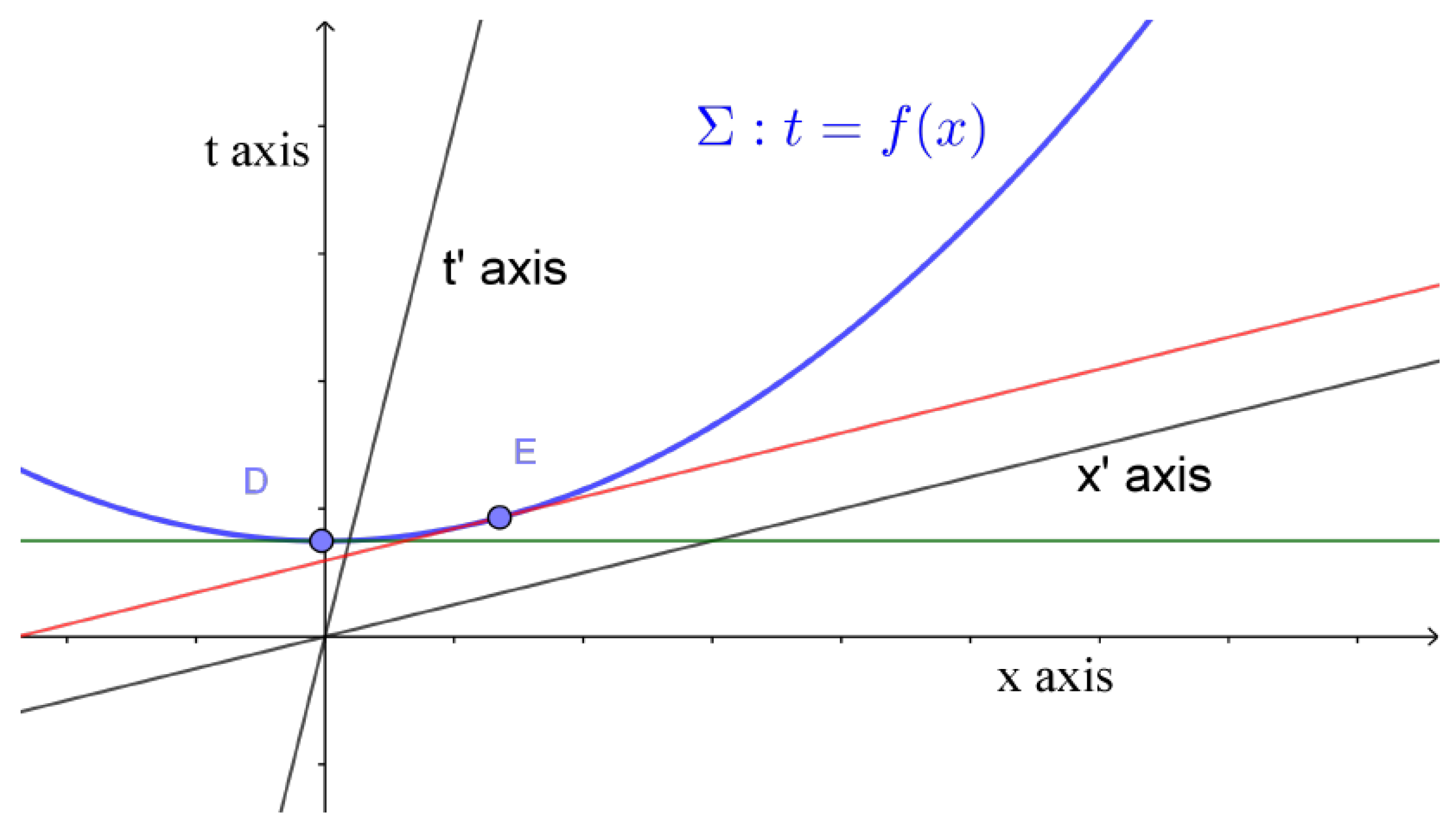
Now, the places where f exhibits an extremum (, point D on Figure 1) do not coincide with those where g does (, point E on Figure 1). The location of the first singularity in the second system (S’) is obtained by solving the equation in (S’); the same spacetime point E would be obtained in (S) by solving in (S). By contrast, in (S), the first singularity D satisfies . The change in the spacetime point where the first singularity is observed may be seen geometrically in one space dimension (see Figure 1). Therefore, the first singularity in (S’) does not correspond to the same spacetime point as the first singularity in (S). The first hot spot in a given inertial system is not the cause of ignition and has no intrinsic physical significance. By contrast, the blow-up set is a well-defined geometric object and its geometric characteristics are physically meaningful.
7. Discussion and Perspectives
7.1. Detonation Signature
The preceding results lead to the identification of combinations of physical quantities that admit limits on the detonation front. Indeed, Theorem 2 shows that the following combinations of the unknowns tend to a finite limit at the singularity (as ):
where the quantities , B and are determined in terms of the arbitrary functions (see Theorems 1 and 2). In particular, when — that is, on the hot spot in the inertial frame at hand —the leading order infinities vanish in the expressions for the density and Eulerian velocities and we obtain the simple result
These limiting behaviors, (26) and (27), give a characteristic signature of this detonation mechanism, that might be tested against measurements.
The fact that the first hot spot is not the cause of ignition is reflected in the fact that is not a constant. The fact that the blow-up pattern is curved in general is reflected in the dependence of the coefficient (in the expansion of the density) on the second-order derivatives of , see (12a) and (13).
A particularly simple limiting behavior is , where, we recall (see (9) and (6)), k only depends on the ratio of specific heats and the length of the gradient of , that is, on the normal velocity in (S) of the detonation front. An overview of measurement techniques may be found in the second chapter of [32]; see also recent papers, such as [6,34].
7.2. Other Asymptotics
In this paper, we assume that the three spatial variables are scaled using the same characteristic length . It would be interesting to introduce different scalings, since some measurements are performed on thin domains, that are essentially two-dimensional [33,34]. The gap width plays the role of a second small parameter, in addition to the inverse activation energy. The detonation signature could exhibit a marked dependence on gap width, which would be consistent with the results of [33,34].
An important application of much current interest is the possibility of introducing ammonia rather than methane in fuel composition, since the former does not contain carbon. The literature is extensive [5,6,7]. This would have obvious advantages from the environmental point of view. It would be of interest to determine the non-dimensional parameters for different fuel compositions.
7.3. Relativistic Effects
The fact that the first hot spot for one observer may not be the first for another is a consequence of the kinematics of special relativity, irrespective of the importance of relativistic effects on the chemistry. This being said, there are two ways to introduce further relativistic effects in this problem. The first is to consider situations in which relativistic effects are significant, as in astrophysics. The second would be to repeat measurements such as those of [33,34] in a moving frame. For instance, one could set the cell used in these measurements in rapid rotation and perform measurements in the (stationary) laboratory frame. One could similarly consider a circular shock tube. Such measurements are perhaps feasible; their interpretation would depend on the importance of inertial effects.
8. Conclusions
(1) When a singularity is formed along a smooth hypersurface of Minkowski spacetime, with an equation of the form , the spacetime location of the first hot spot is not a Lorentz invariant. This is a consequence of the Lorentz transformation between observers in special relativity and is independent of the size of the relativistic effects in the modeling of the physical situation that led to singularity-formation. However, the set of all singularities seen by all observers is a well-defined geometric object—the blow-up set.
(2) These ideas apply to the weak detonation problem. We have solved the appropriate system of PDEs, in the limit of high activation energy, by integrating them from singularity data given on the blow-up set, or detonation locus, and obtained a general solution of the equations. It contains the maximum number of arbitrary functions, namely, five. This solution improves earlier results in three respects: (i) It provides a description of the solution that is valid when it is large, but not infinite; in the weak detonation problem, the temperature never becomes actually infinite. (ii) It identifies which combinations of physical quantities remain finite at blow-up. (iii) It takes into account the kinematics of special relativity.
(3) In addition, the arbitrary functions in the general solution admit a physical interpretation in terms of the behavior of density, velocity and temperature at the singularity. This provides a signature for this type of ignition mechanism.
(4) Perspectives include the following: (i) a similar asymptotic study for nearly two-dimensional situations used in some measurements; (ii) the measurement of a detonation signature on the basis of the limiting behavior of the physical quantities, including the curvature of the blow-up pattern; (iii) the inclusion of the relativistic effects in the chemistry; (iv) the impact of fuel composition, especially the inclusion of hydrogen or ammonia in the mix, on the non-dimensional parameters, therefore on the domain of validity of this ignition mechanism.
Funding
This research was partially funded by CNRS through its research group UMR9008 in Reims. The APC was waived by MDPI.
Institutional Review Board Statement
Not applicable.
Informed Consent Statement
Not applicable.
Acknowledgments
The author thanks Leila Zhang at MDPI for encouraging him to prepare and submit this paper, and the referees for their kind comments.
Conflicts of Interest
The author declares no conflict of interest. The funders had no role in the design of the study; in the collection, analyses, or interpretation of data; in the writing of the manuscript, or in the decision to publish the results.
Appendix A. Derivation of the Basic System
Let us consider a reactive fluid, with reactant mass fraction y (i.e., one gram of fluid contains y grams of reactant and grams of reaction products). The overall reaction is modeled by a one-step irreversible reaction in the form , where the reactant and the product have the same specific heats and , as well as the same molar mass . This makes it possible to consider and as forming a single perfect fluid, with density , specific volume , Eulerian velocity , pressure p and temperature T, that all vary with in space and time. Therefore, the equation of state is
where R is the perfect gas constant, , and
The specific internal energy is
where the constant q is the heat release rate. The total specific energy is
where . The reaction rate is given by the Arrhenius law
where A and E are constants.
To write the conservation laws, let us introduce the material derivative operator
Mass, momentum and energy conservation read
By (A2a), . Therefore,
In addition, . On the other hand,
Therefore, Equation (A2c) takes the form
Using the Arrhenius law,
To sum up, we have to solve the following system:
The objective is to solve this system in the limit when the activation energy E is large.
Appendix B. Non-Dimensionalization
Appendix B.1. Non-Dimensional Variables
Let us introduce a reference state characterized by the values , , and , a reference length and reference time . They determine . We introduce scaled variables by
We take and assume the equation of state holds for the reference state . The velocity determines the acoustic time . The main non-dimensional parameters for the present analysis are
Appendix B.2. Choice of Time and Length Scales
The modeling assumptions (A2–A4) translate into the following choices:
- Fix the reference time by .
- Fix the reference length so that . That means , or .
To express the compatibility of these assumptions, we relate M and . First,
Therefore, since ,
The assumptions and are compatible if is large; this is consistent with the assumption that the reaction is strongly exothermic. Additionally, since for , the reaction proceeds slowly with respect to the reference time scale .
With these assumptions, the dimensionless equations become
References
- Lee, J.H.S. The Detonation Phenomenon; Cambridge University Press: New York, NY, USA, 2008. [Google Scholar]
- Sivashinsky, G.I. Some developments in premixed combustion modeling. Proc. Combust. Inst. 2002, 29, 1737–1761. [Google Scholar] [CrossRef]
- Urtiew, P.A.; Oppenheim, A.K. Experimental observations of the transition to detonation in an explosive gas. Proc. R. Soc. Lond. A 1966, 295, 13–28. [Google Scholar]
- Williams, F.A. Combustion Theory; Addison-Wesley: Reading, MA, USA, 1985. [Google Scholar]
- Hasan, M.H.; Mahlia, T.M.I.; Mofijur, M.; Rizwanul Fattah, I.M.; Handayani, F.; Ong, H.C.; Silitonga, A.S. A comprehensive review on the recent development of ammonia as a renewable energy carrier. Energies 2021, 14, 3732. [Google Scholar] [CrossRef]
- Tang, G.; Jin, P.; Bao, Y.; Chai, W.S.; Zhou, L. Experimental investigation of premixed combustion limits of hydrogen and methane additives in ammonia. Int. J. Hydrogen Energy 2021, 46, 20765–20776. [Google Scholar] [CrossRef]
- Valera-Medina, A.; Xiao, H.; Owen-Jones, M.; David, W.I.F.; Bowen, P.J. Ammonia for power. Prog. Energy Combust. Sci. 2018, 69, 63–102. [Google Scholar] [CrossRef]
- Kichenassamy, S. Fuchsian Reduction: Applications to Geometry, Cosmology and Mathematical Physics; Birkhäuser: Boston, MA, USA, 2007. [Google Scholar]
- Kichenassamy, S. Stability of blow-up patterns for nonlinear wave equations. In Nonlinear PDEs, Dynamics and Continuum Physics; Bona, J., Saxton, K.R., Eds.; AMS: Providence, RI, USA, 2000; pp. 139–162. [Google Scholar]
- Kichenassamy, S.; Littman, W. Blow-up surfaces for nonlinear wave equations, I & II. Commun. Partial Differ. Equ. 1993, 18. 431–452 and 1869–1899. [Google Scholar]
- Kichenassamy, S. Control of blow-up singularities for nonlinear wave equations, Evol. Equ. Control Theory 2013, 2, 667–677. [Google Scholar]
- Cabart, G.; Kichenassamy, S. Explosion et normes Lp pour l’équation des ondes non linéaire cubique. Comptes Rendus Math. 2002, 335, 903–908. [Google Scholar]
- Kapila, A.K.; Jackson, T.L. Dynamics of hot-spot evolution in a reactive, compressible flow. In Computational Fluid Dynamics and Reacting Gas Flows; IMA Volumes in Mathematics and its Applcations 12; Engquist, B., Luskin, M., Majda, A., Eds.; Springer: Boston, MA, USA, 1988; pp. 123–150. [Google Scholar]
- Blythe, P.A.; Crighton, D.G. Shock-generated ignition: The induction zone. Proc. R. Soc. Lond. A 1989, 426, 189–209. [Google Scholar]
- Clarke, J.F.; Cant, R.S. Non-steady gasdynamic effects in the induction domain behind a strong shock wave. In Dynamics of Flames and Reactive Systems; Progress in Astronautics and Aeronautics 95; Bowen, J.R., Manson, N., Oppenheim, A.K., Eds.; American Institute of Aeronautics: New York, NY, USA, 1984; pp. 142–163. [Google Scholar]
- Jackson, T.L.; Kapila, A.K.; Stewart, D.S. Evolution of a reaction center in an explosive material. SIAM J. Appl. Math. 1989, 49, 432–458. [Google Scholar] [CrossRef]
- Campbell, A.W.; Davis, W.C.; Travis, J.R. Shock initiation of detonation in liquid explosives. Phys. Fluids 1961, 4, 498–510. [Google Scholar] [CrossRef]
- Clarke, J.F. Propagation of gas dynamic disturbance in an explosive atmosphere. Prog. Astronaut. Aeronaut. 1981, 76, 383–402. [Google Scholar]
- Dold, J.W.; Kapila, A.K.; Short, M. Theoretical description of direct initiation of detonation for one-step chemistry. In Dynamic Structure of Detonation in Gaseous and Dispersed Media; Borisov, A.A., Ed.; Kluwer: Dordrecht, The Netherlands, 1991; pp. 245–256. [Google Scholar]
- Dremin, A.N. Toward Detonation Theory; Springer: Berlin, Germany, 1999. [Google Scholar]
- Fickett, W.; Davis, W.C. Detonation: Theory and Experiment; Dover: Mineola, NY, USA, 2000. [Google Scholar]
- Jackson, T.L.; Kapila, A.K. Shock-induced thermal runaway. SIAM J. Appl. Math. 1985, 45, 130–137. [Google Scholar] [CrossRef]
- Kapila, A.K.; Dold, J.W. A theoretical picture of shock-to-detonation transition in a homogeneous explosive. In 9th Symposium (International) on Detonation; OCNR 113291-7; Office of Naval Research: Washington, DC, USA, 1989; pp. 219–227. [Google Scholar]
- Kassoy, D.R. Extremely rapid transient phenomona in combustion, ignition and explosion. In Asymptotic Methods and Singular Perturbations; SIAM-AMS Proc; O’Malley, R.E., Ed.; AMS: Providence, RI, USA, 1976; Volume 10, pp. 61–72. [Google Scholar]
- Meyer, J.W.; Oppenheim, A.K. Dynamic response of a plane-symmetrical exothermic reaction center. AIAA J. (Publ. Am. Inst. Aeronaut. Astronaut.) 1972, 10, 1509–1513. [Google Scholar] [CrossRef]
- Poland, J.; Kassoy, D.R. The induction period of a thermal explosion in a gas between infinite parallel plates. Combust. Flame 1983, 50, 259–274. [Google Scholar] [CrossRef]
- Shepherd, J.E. Detonation in gases. Proc. Combust. Inst. 2009, 32, 83–98. [Google Scholar] [CrossRef]
- Short, M. On the critical conditions for the initiation of a detonation in a nonuniformly perturbed reactive fluid. SIAM J. Appl. Math. 1997, 57, 1242–1280. [Google Scholar] [CrossRef]
- Short, M.; Dold, J.W. Weak detonations, their paths and transition to strong detonation. Combust. Theory Modeling 2002, 6, 279–296. [Google Scholar] [CrossRef] [Green Version]
- Zajac, L.J.; Oppenheim, A.K. Dynamics of an explosive reaction center. AIAA J. (Publ. Am. Inst. of Aeronaut. Astronaut.) 1971, 9, 545–553. [Google Scholar] [CrossRef]
- Kichenassamy, S. The blow-up problem for exponential nonlinearities. Commun. Partial Differ. Equ. 1996, 21, 125–162. [Google Scholar] [CrossRef] [Green Version]
- Warnatz, J.; Maas, U.; Dibble, R.W. Combustion—Physical and Chemical Foundations, Modeling and Simulation, Experiments, Pollutant Formation, 3rd ed.; Springer: Berlin, Germany, 2001. [Google Scholar]
- Wu, M.-H.; Kuo, W.-C. Accelerative expansion and DDT of stoichiometric ethylene/oxygen flame rings in microgaps. Proc. Combust. Inst. 2013, 34, 2017–2024. [Google Scholar] [CrossRef]
- Ssu, H.-W.; Wu, M.-H. Formation and characteristics of composite reaction—Shock clusters in narrow channels. Proc. Combust. Inst. 2021, 28, 3473–3480. [Google Scholar] [CrossRef]
Figure 1.
Illustration of the transformation of the first hot spot under a Lorentz transformation. The singular set (in blue) has equation in a two-dimensional Minkowski space, for an observer with rectangular coordinates . The time of the first singularity corresponds, for this observer, to the spacetime point D. For another inertial observer, his/her time and space axes are slanted lines, as indicated, and the first singularity is observed at a different spacetime point E, that may be constructed by finding the tangent to (in red) parallel to the -axis.

Publisher’s Note: MDPI stays neutral with regard to jurisdictional claims in published maps and institutional affiliations. |
© 2021 by the author. Licensee MDPI, Basel, Switzerland. This article is an open access article distributed under the terms and conditions of the Creative Commons Attribution (CC BY) license (https://creativecommons.org/licenses/by/4.0/).
Share and Cite
MDPI and ACS Style
Kichenassamy, S. Hot Spots in the Weak Detonation Problem and Special Relativity. Axioms 2021, 10, 311. https://doi.org/10.3390/axioms10040311
AMA Style
Kichenassamy S. Hot Spots in the Weak Detonation Problem and Special Relativity. Axioms. 2021; 10(4):311. https://doi.org/10.3390/axioms10040311
Chicago/Turabian StyleKichenassamy, Satyanad. 2021. "Hot Spots in the Weak Detonation Problem and Special Relativity" Axioms 10, no. 4: 311. https://doi.org/10.3390/axioms10040311
Note that from the first issue of 2016, this journal uses article numbers instead of page numbers. See further details here.