Article

Constructing a Precise Fuzzy Feedforward Neural Network Using an Independent Fuzzification Approach

1
Department of Industrial Engineering and Management, Chaoyang University of Science and Technology, Taichung 413310, Taiwan
2
Department of Industrial Engineering and Management, National Yang Ming Chiao Tung University, 1001, University Road, Hsinchu 30010, Taiwan
3
Department of Industrial Engineering and Management, National Chin-Yi University of Technology, Taichung 411030, Taiwan
*
Author to whom correspondence should be addressed.
Axioms 2021, 10(4), 282; https://doi.org/10.3390/axioms10040282
Submission received: 8 October 2021 / Revised: 25 October 2021 / Accepted: 26 October 2021 / Published: 28 October 2021
(This article belongs to the Special Issue Intelligent and Fuzzy Systems)

Abstract

:
This study discusses how to fuzzify a feedforward neural network (FNN) to generate a fuzzy forecast that contains the actual value, while minimizing the average range of fuzzy forecasts. This topic has rarely been investigated in past studies, but is an essential step to constructing a precise fuzzy FNN (FFNN). Existing methods fuzzify all parameters at the same time, which re-sults in a nonlinear programming (NLP) problem that is not easy to solve. In contrast, in this study, the parameters of a FNN are fuzzified independently. In this way, the optimal values of fuzzy parameters can be derived theoretically. An illustrative example is used to illustrate the ap-plicability of the proposed methodology. According to the experimental results, fuzzifying the thresholds on hidden-layer nodes or the connection weights between input and hidden layers may not guarantee that all fuzzy forecasts contain the corresponding actual values. In contrast, fuzzi-fying the threshold on the output node and the connection weights between the hidden and out-put layers is more likely to achieve a 100% hit rate. The results lay a foundation for establishing a precise deep FFNN in the future.

1. Introduction

Fuzzy feedforward neural networks (FFNNs) combines the advantages of fuzzy logic (in uncertainty modelling) and feedforward neural networks (FNNs) (in nonlinear approximation) [1], and have been widely applied to forecasting in many fields [2,3,4,5]. There are various types of FFNNs with fuzzy or crisp inputs, parameters, and outputs. The numbers of layers and activation (or transformation) functions in these FFNNs are also different [6]. A recent review on FFNNs refers to de Campos Souza [7]. At present, the most commonly applied FFNNs are the variants of adaptive network-based fuzzy inference system (ANFIS) [8,9,10,11,12,13]. Past studies have shown that FFNNs can improve the forecasting accuracy, that is, each forecast is close to the actual value [14,15,16]. However, the present study aims to construct an FFNN to improve the forecasting precision, that is, every actual value is included in the narrowest possible fuzzy forecast. This topic has rarely been discussed in the past, which constitutes the motivation of this research.
However, even if a sophisticated FFNN is applied, the network output is rarely equal to the actual value, especially when the FFNN is applied to unlearned data. To address this issue, an alternative is to estimate the range of the actual value [17]. In other words, a fuzzy forecast that contains the actual value needs to be generated by an FFNN, at least for the training data. However, it is not easy since there are no actual values of the lower and upper bounds of the range. In addition, a fuzzy forecast needs to be as narrow as possible to have a reference value [18]. This is also a challenging task because a narrower range is less likely to contain the actual value. Some of the relevant literature are reviewed as follows.
In an ANFIS, the network output before defuzzification cannot guarantee the inclusion of the actual value [19]. The problem is even more complicated for an FFNN in which all parameters are fuzzy and nonlinear transformation functions (such as sigmoid or tansig functions) are applied. For example, Chen and Wang [20] showed that the problem of deriving the values of fuzzy parameters in an FFNN was a nonlinear programming (NLP) problem that was difficult to solve. A branch-and-bound algorithm can be applied to find a solution to the NLP problem [21], but the solution may be far from (global) optimal. Instead, Chen and Wang established goals for the lower and upper bounds of the actual value to simplify the NLP problem to a goal programming (GP) problem. However, a number of goals needed to be tried to improve the solution, which was time-consuming. A similar method was proposed in Chen and Lin [18], in which the membership of an actual value in the fuzzy forecast had to be greater than a specified level. If only the threshold on the output node was fuzzy, the optimal value of the fuzzy threshold can be derived by solving two linear equations [22]. Similar treatments have been taken by Chen and Wu [17] and Chen [23]. Wang et al. [24] randomized the values of fuzzy thresholds on hidden-layer nodes and then optimized the fuzzy threshold on the output node. After a few replications, these fuzzy thresholds could be optimized. However, connection weights in the FFNN were still crisp.
This study considers an FFNN with a single hidden layer in which all network parameters can be fuzzified and nonlinear transformation functions (i.e., sigmoid functions) are adopted. We aim to optimize the values of fuzzy parameters theoretically without solving an NLP problem, while guaranteeing that all actual values are contained in the corresponding fuzzy forecasts. However, instead of fuzzifying all parameters at the same time, this study follows an independent fuzzification approach in which parameters are fuzzified independently. This study is important because it is a fundamental step towards the construction of a precise FFNN, which lays a foundation for establishing a precise deep FFNN with multiple or recurrent hidden layers.
The contribution of this research is to derive the formula for optimizing the value of each fuzzy parameter in an FFNN, so as to minimize the average range of fuzzy forecasts while ensuring a 100% hit rate. In contrast, existing methods need to solve an NLP problem to achieve the same goal.
The remainder of this study is organized as follows. The independent fuzzification approach is detailed in Section 2. A numerical example is given in Section 3 to illustrate the applicability of the proposed methodology. The effects of fuzzifying various parameters on the average range of fuzzy forecasts are also compared. This study is concluded in Section 4. Some directions for future investigation are also provided.

2. Independent Fuzzification Approach

All parameters and variables in the proposed methodology are given in or approximated by triangular fuzzy numbers (TFNs).

2.1. FFNN Configuration

The FFNN considered in this study is an FFNN that has three layers: the input layer, a single hidden layer, and the output layer. Inputs to the FFNN are indicated with { z j p | p = 1~P; j = 1~n}. z j p is the normalized value of decision variable x j p :
z j p = x j p min v x v p max v x v p min v x v p
To convert back to the original value,
x j p = U ( z j p ) = z j p ( max v x v p min v x v p ) + min v x v p
These inputs are propagated through the FFNN as follows. First, from the input layer to the hidden layer, the following operations are performed:
I ˜ j l h = p = 1 P ( w ˜ p l h z j p )
n ˜ j l h = I ˜ j l h ( ) θ ˜ l h = ( I j l 1 h θ l 3 h , I j l 2 h θ l 2 h , I j l 3 h θ l 1 h )
h ˜ j l = 1 1 + e n ˜ j l h
where w ˜ p l h is the connection weight between input node p and hidden-layer node l; l = 1~L. θ ˜ l h is the threshold on hidden-layer node l. h ˜ j l is the output from hidden-layer node l. (−) denotes fuzzy subtraction. In Equation (5), the activation (or transformation) function is the logistic sigmoid activation function that returns a value within [0, 1].
Outputs from the hidden layer are aggregated on the output node,
I ˜ j o = l = 1 L ( w ˜ l o ( × ) h ˜ j l )
and then the network output o ˜ j = ( o j 1 , o j 2 , o j 3 ) is generated as
o ˜ j = 1 1 + e n ˜ j o
where
n ˜ j o = I ˜ j o ( ) θ ˜ o
w ˜ l o is the connection weight between hidden-layer node l and the output node. θ ˜ o is the threshold on the output node. o ˜ j is unnormalized according to Equation (2) and then compared with the actual value y j .

2.2. Deriving the Cores of Fuzzy Parameters

The training of the FFNN is composed of two stages. First, the cores of fuzzy parameters are derived by training the FFNN as a crisp FNN using the Levenberg–Marquardt (LM) algorithm [25], so as to minimize the mean squared error (MSE). The optimal solution is indicated with { w p l 2 h * , θ l 2 h * , w l 2 o * , θ 2 o * | p = 1~P; l = 1~L}.
Subsequently, the lower and upper bounds of fuzzy parameters are to be determined, so as to minimize the average range (AR) of fuzzy forecasts:
Min   A R = 1 n j = 1 n ( o j 3 o j 1 )
However, deriving the optimal values of all fuzzy parameters at the same time is a computationally intensive task [20]. As an alternative, the optimal values of fuzzy parameters are derived independently as follows.

2.3. Deriving the Optimal Value of θ ˜ o

The optimal value of θ ˜ o is to be derived. First, substituting Equation (8) into Equation (7) gives
o ˜ j = 1 1 + e ( θ ˜ o ( ) I ˜ j o )
which can be decomposed into
o j 1 = 1 1 + e ( θ 3 o I j 1 o )
o j 3 = 1 1 + e ( θ 1 o I j 3 o )
The other parameters are not fuzzified, so I j 1 o and I j 3 o are equal to I j 2 o * that is a fixed value:
o j 1 = 1 1 + e ( θ 3 o I j 2 o * )
o j 3 = 1 1 + e ( θ 1 o I j 2 o * )
To minimize AR, o j 1 and o j 3 should be maximized and minimized, respectively, which correspond to the minimization of θ 3 o and the maximization of θ 1 o . However, o ˜ j should include a j (the actual value), therefore
o j 1 a j ;   j   =   1   ~   n
o j 3 a j ;   j   =   1   ~   n
In addition, o j 1 o j 2 * o j 3 , so
o j 1 min ( o j 2 * , a j ) ;   j   =   1   ~   n
o j 3 max ( o j 2 * , a j ) ;   j   =   1   ~   n
Substituting Equation (13) into Constraint (17) gives
θ 3 o I j 2 o * + ln ( 1 min ( o j 2 * , a j ) 1 ) ;   j   =   1   ~   n
Therefore,
θ 3 o max j I j 2 o * + ln ( 1 min ( o j 2 * , a j ) 1 )
To minimize θ 3 o ,
θ 3 o * = max j I j 2 o * + ln ( 1 min ( o j 2 * , a j ) 1 )
Similarly, by substituting Equation (14) into Constraint (18), the following result can be obtained:
θ 1 o * = min j I j 2 o * + ln ( 1 max ( o j 2 * , a j ) 1 )
Most past studies [17,22,23,24] stop at this step. The following discussion is new to the body of knowledge.

2.4. Deriving the Optimal Value of w ˜ l f o

The optimal value of w ˜ l o is to be derived when l = l f . Equation (6) can be decomposed into
I j 1 o = min l = 1 L ( w l 1 o h j l 1 ) , l = 1 L ( w l 1 o h j l 3 )
I j 3 o = max l = 1 L ( w l 3 o h j l 1 ) , l = 1 L ( w l 3 o h j l 3 )
because h ˜ j l is positive, while w ˜ l o may be negative. Substituting Equations (23) and (24) into Equations (13) and (14) gives
o j 1 = 1 1 + e θ 3 o min ( l = 1 L ( w l 1 o h j l 1 ) , l = 1 L ( w l 1 o h j l 3 ) )
o j 3 = 1 1 + e θ 1 o max ( l = 1 L ( w l 3 o h j l 1 ) , l = 1 L ( w l 3 o h j l 3 ) )
Only connection weights are fuzzified. The other fuzzy parameters are set to their optimized cores as
o j 1 = 1 1 + e θ 2 o * min ( l = 1 L ( w l 1 o h j l 2 * ) , l = 1 L ( w l 1 o h j l 2 * ) ) = 1 1 + e θ 2 o * l = 1 L ( w l 1 o h j l 2 * )
o j 3 = 1 1 + e θ 2 o * max ( l = 1 L ( w l 3 o h j l 2 * ) , l = 1 L ( w l 3 o h j l 2 * ) ) = 1 1 + e θ 2 o * l = 1 L ( w l 3 o h j l 2 * )
Substituting Equations (27) and (28) respectively into Constraints (17) and (18), we obtain
l = 1 L ( w l 1 o h j l 2 * ) θ 2 o * ln ( 1 min ( o j 2 * , a j ) 1 ) ;   j   =   1   ~   n
l = 1 L ( w l 3 o h j l 2 * ) θ 2 o * ln ( 1 max ( o j 2 * , a j ) 1 ) ;   j   =   1   ~   n
Only w l f o is fuzzified, the other connection weights are equal to their optimized cores:
w l f 1 o h j l f 2 * + l l f ( w l 2 o * h j l 2 * ) θ 2 o * ln ( 1 min ( o j 2 * , a j ) 1 ) ;   j   =   1   ~   n
w l f 3 o h j l f 2 * + l l f ( w l 2 o * h j l 2 * ) θ 2 o * ln ( 1 max ( o j 2 * , a j ) 1 ) ;   j   =   1   ~   n
As a result,
w l f 1 o θ 2 o * ln ( 1 min ( o j 2 * , a j ) 1 ) l l f ( w l 2 o * h j l 2 * ) h j l f 2 * ;   j   =   1   ~   n
w l f 3 o θ 2 o * ln ( 1 max ( o j 2 * , a j ) 1 ) l l f ( w l 2 o * h j l 2 * ) h j l f 2 * ;   j   =   1   ~   n
Therefore,
w l f 1 o min j θ 2 o * ln ( 1 min ( o j 2 * , a j ) 1 ) l l f ( w l 2 o * h j l 2 * ) h j l f 2 *
w l f 3 o max j θ 2 o * ln ( 1 max ( o j 2 * , a j ) 1 ) l l f ( w l 2 o * h j l 2 * ) h j l f 2 *
Increasing the fuzziness (i.e., width) of w ˜ l f o will make o ˜ j wider. Therefore, it is reasonable to set
w l f 1 o * = min j θ 2 o * ln ( 1 min ( o j 2 * , a j ) 1 ) l l f ( w l 2 o * h j l 2 * ) h j l f 2 *
w l f 3 o * = max j θ 2 o * ln ( 1 max ( o j 2 * , a j ) 1 ) l l f ( w l 2 o * h j l 2 * ) h j l f 2 *

2.5. Deriving the Optimal Value of θ ˜ l h

Substituting Equation (4) into Equation (5) gives
h ˜ j l = 1 1 + e ( θ ˜ l h ( ) I ˜ j l h )
which can be decomposed into
h j l 1 = 1 1 + e ( θ l 3 h I j l 1 h )
h j l 3 = 1 1 + e ( θ l 1 h I j l 3 h )
Substituting Equations (40) and (41) into Equations (23) and (24) leads to
I j 1 o = min l = 1 L w l 1 o 1 + e ( θ l 3 h I j l 1 h ) , l = 1 L w l 1 o 1 + e ( θ l 1 h I j l 3 h )
I j 3 o = max l = 1 L w l 3 o 1 + e ( θ l 3 h I j l 1 h ) , l = 1 L w l 3 o 1 + e ( θ l 1 h I j l 3 h )
that are substituted into Equations (13) and (14):
o j 1 = 1 1 + e θ 3 o min l = 1 L w l 1 o 1 + e ( θ l 3 h I j l 1 h ) , l = 1 L w l 1 o 1 + e ( θ l 1 h I j l 3 h )
o j 3 = 1 1 + e θ 1 o max l = 1 L w l 3 o 1 + e ( θ l 3 h I j l 1 h ) , l = 1 L w l 3 o 1 + e ( θ l 1 h I j l 3 h )
The following requirements should be met:
1 1 + e θ 3 o min l = 1 L w l 1 o 1 + e ( θ l 3 h I j l 1 h ) , l = 1 L w l 1 o 1 + e ( θ l 1 h I j l 3 h ) min ( o j 2 * , a j ) ;   j   =   1   ~   n
1 1 + e θ 1 o max l = 1 L w l 3 o 1 + e ( θ l 3 h I j l 1 h ) , l = 1 L w l 3 o 1 + e ( θ l 1 h I j l 3 h ) max ( o j 2 * , a j ) ;   j   =   1   ~   n
that are equivalent to
min l = 1 L w l 1 o 1 + e ( θ l 3 h I j l 1 h ) , l = 1 L w l 1 o 1 + e ( θ l 1 h I j l 3 h ) θ 3 o ln ( 1 min ( o j 2 * , a j ) 1 ) ;   j   =   1   ~   n
max l = 1 L w l 3 o 1 + e ( θ l 3 h I j l 1 h ) , l = 1 L w l 3 o 1 + e ( θ l 1 h I j l 3 h ) θ 1 o ln ( 1 max ( o j 2 * , a j ) 1 ) ;   j   =   1   ~   n
Only θ l f h is fuzzified, the other fuzzy parameters are set to their optimized cores:
min w l f 2 o * 1 + e ( θ l f 3 h I j l f 2 h * ) + l l f w l 2 o * 1 + e ( θ l 2 h * I j l 2 h * ) , w l f 2 o * 1 + e ( θ l f 1 h I j l f 2 h * ) + l l f w l 2 o * 1 + e ( θ l 2 h * I j l 2 h * ) θ 2 o * ln ( 1 min ( o j 2 * , a j ) 1 ) ;   j   =   1   ~   n
max w l f 2 o * 1 + e ( θ l f 3 h I j l f 2 h * ) + l l f w l 2 o * 1 + e ( θ l 2 h * I j l 2 h * ) , w l f 2 o * 1 + e ( θ l f 1 h I j l f 2 h * ) + l l f w l 2 o * 1 + e ( θ l 2 h * I j l 2 h * ) θ 2 o * ln ( 1 max ( o j 2 * , a j ) 1 ) ;   j   =   1   ~   n
If w l f 2 o * 0 ,
w l f 2 o * 1 + e ( θ l f 3 h I j l f 2 h * ) + l l f w l 2 o * 1 + e ( θ l 2 h * I j l 2 h * ) θ 2 o * ln ( 1 min ( o j 2 * , a j ) 1 ) ;   j   =   1   ~   n
w l f 2 o * 1 + e ( θ l f 1 h I j l f 2 h * ) + l l f w l 2 o * 1 + e ( θ l 2 h * I j l 2 h * ) θ 2 o * ln ( 1 max ( o j 2 * , a j ) 1 ) ;   j   =   1   ~   n
As a result,
θ l f 3 h ln ( w l f 2 o * θ 2 o * ln ( 1 min ( o j 2 * , a j ) 1 ) l l f w l 2 o * 1 + e ( θ l 2 h * I j l 2 h * ) 1 ) + I j l f 2 h * ;   j   =   1   ~   n
θ l f 1 h ln ( w l f 2 o * θ 2 o * ln ( 1 max ( o j 2 * , a j ) 1 ) l l f w l 2 o * 1 + e ( θ l 2 h * I j l 2 h * ) 1 ) + I j l f 2 h * ;   j   =   1   ~   n
Therefore,
θ l f 1 h min j ln ( w l f 2 o * θ 2 o * ln ( 1 max ( o j 2 * , a j ) 1 ) l l f w l 2 o * 1 + e ( θ l 2 h * I j l 2 h * ) 1 ) + I j l f 2 h *
θ l f 3 h max j ln ( w l f 2 o * θ 2 o * ln ( 1 min ( o j 2 * , a j ) 1 ) l l f w l 2 o * 1 + e ( θ l 2 h * I j l 2 h * ) 1 ) + I j l f 2 h *
To minimize the fuzziness of θ ˜ l f h ,
θ l f 1 h * = min j ln ( w l f 2 o * θ 2 o * ln ( 1 max ( o j 2 * , a j ) 1 ) l l f w l 2 o * 1 + e ( θ l 2 h * I j l 2 h * ) 1 ) + I j l f 2 h *
θ l f 3 h * = max j ln ( w l f 2 o * θ 2 o * ln ( 1 min ( o j 2 * , a j ) 1 ) l l f w l 2 o * 1 + e ( θ l 2 h * I j l 2 h * ) 1 ) + I j l f 2 h *
Otherwise,
w l f 2 o * 1 + e ( θ l f 1 h I j l f 2 h * ) + l l f w l 2 o * 1 + e ( θ l 2 h * I j l 2 h * ) θ 2 o * ln ( 1 min ( o j 2 * , a j ) 1 ) ;   j   =   1   ~   n
w l f 2 o * 1 + e ( θ l f 3 h I j l f 2 h * ) + l l f w l 2 o * 1 + e ( θ l 2 h * I j l 2 h * ) θ 2 o * ln ( 1 max ( o j 2 * , a j ) 1 ) ;   j   =   1   ~   n
As a result,
θ l f 1 h ln ( w l f 2 o * θ 2 o * ln ( 1 min ( o j 2 * , a j ) 1 ) l l f w l 2 o * 1 + e ( θ l 2 h * I j l 2 h * ) 1 ) + I j l f 2 h * ;   j   =   1   ~   n
θ l f 3 h ln ( w l f 2 o * θ 2 o * ln ( 1 max ( o j 2 * , a j ) 1 ) l l f w l 2 o * 1 + e ( θ l 2 h * I j l 2 h * ) 1 ) + I j l f 2 h * ;   j   =   1   ~   n
Therefore,
θ l f 1 h max j ln ( w l f 2 o * θ 2 o * ln ( 1 min ( o j 2 * , a j ) 1 ) l l f w l 2 o * 1 + e ( θ l 2 h * I j l 2 h * ) 1 ) + I j l f 2 h *
θ l f 3 h min j ln ( w l f 2 o * θ 2 o * ln ( 1 max ( o j 2 * , a j ) 1 ) l l f w l 2 o * 1 + e ( θ l 2 h * I j l 2 h * ) 1 ) + I j l f 2 h *
To minimize the fuzziness of θ ˜ l f h , θ l f 1 h * and θ l f 3 h * should be maximized and minimized, respectively, but they are still bounded by θ l f 2 h * . Therefore,
θ l f 1 h * = θ l f 2 h *
θ l f 3 h * = θ l f 2 h *

2.6. Deriving the Optimal Value of w ˜ p l h

Equation (3) can be decomposed into
I j l 1 h = p = 1 P ( w p l 1 h z j p )
I j l 3 h = p = 1 P ( w p l 3 h z j p )
Substituting Equations (68) and (69) into Equations (46) and (47) gives
o j 1 = 1 1 + e θ 3 o min l = 1 L w l 1 o 1 + e ( θ l 3 h p = 1 P ( w p l 1 h z j p ) ) , l = 1 L w l 1 o 1 + e ( θ l 1 h p = 1 P ( w p l 3 h z j p ) )
o j 3 = 1 1 + e θ 1 o max l = 1 L w l 3 o 1 + e ( θ l 3 h p = 1 P ( w p l 1 h z j p ) ) , l = 1 L w l 3 o 1 + e ( θ l 1 h p = 1 P ( w p l 3 h z j p ) )
The following requirements need to be met:
1 1 + e θ 3 o min l = 1 L w l 1 o 1 + e ( θ l 3 h p = 1 P ( w p l 1 h z j p ) ) , l = 1 L w l 1 o 1 + e ( θ l 1 h p = 1 P ( w p l 3 h z j p ) ) min ( o j 2 * , a j ) ;   j   =   1   ~   n
1 1 + e θ 1 o max l = 1 L w l 3 o 1 + e ( θ l 3 h p = 1 P ( w p l 1 h z j p ) ) , l = 1 L w l 3 o 1 + e ( θ l 1 h p = 1 P ( w p l 3 h z j p ) ) max ( o j 2 * , a j ) ;   j   =   1   ~   n
that are equivalent to
min l = 1 L w l 1 o 1 + e ( θ l 3 h p = 1 P ( w p l 1 h x j p ) ) , l = 1 L w l 1 o 1 + e ( θ l 1 h p = 1 P ( w p l 3 h x j p ) ) θ 3 o ln ( 1 min ( o j 2 * , a j ) 1 ) ;   j   =   1   ~   n
max l = 1 L w l 3 o 1 + e ( θ l 3 h p = 1 P ( w p l 1 h x j p ) ) , l = 1 L w l 3 o 1 + e ( θ l 1 h p = 1 P ( w p l 3 h x j p ) ) θ 1 o ln ( 1 max ( o j 2 * , a j ) 1 ) ;   j   =   1   ~   n
Only w p f l f h is fuzzified, the other fuzzy parameters are set to their optimized cores:
min w l f 2 o * 1 + e ( θ l f 2 h * w p f l f 1 h x j p f p p f ( w p l f 2 h * x j p ) ) + l l f w l 2 o * 1 + e ( θ l 2 h * p = 1 P ( w p l 2 h * x j p ) ) , w l f 2 o * 1 + e ( θ l f 2 h * w p f l f 3 h x j p f p p f ( w p l f 2 h * x j p ) ) + l l f w l 2 o * 1 + e ( θ l 2 h * p = 1 P ( w p l 2 h * x j p ) ) θ 2 o * ln ( 1 min ( o j 2 * , a j ) 1 ) ;   j   =   1   ~   n
max w l f 2 o * 1 + e ( θ l f 2 h * w p f l f 1 h x j p f p p f ( w p l f 2 h * x j p ) ) + l l f w l 2 o * 1 + e ( θ l 2 h * p = 1 P ( w p l 2 h * x j p ) ) , w l f 2 o * 1 + e ( θ l f 2 h * w p f l f 3 h x j p f p p f ( w p l f 2 h * x j p ) ) + l l f w l 2 o * 1 + e ( θ l 2 h * p = 1 P ( w p l 2 h * x j p ) ) θ 2 o * ln ( 1 max ( o j 2 * , a j ) 1 ) ;   j   =   1   ~   n
If w l f 2 o * 0 ,
w l f 2 o * 1 + e ( θ l f 2 h * w p f l f 3 h x j p f p p f ( w p l f 2 h * x j p ) ) + l l f w l 2 o * 1 + e ( θ l 2 h * p = 1 P ( w p l 2 h * x j p ) ) θ 2 o * ln ( 1 max ( o j 2 * , a j ) 1 ) ;   j   =   1   ~   n
As a result,
w p f l f 1 h θ l f 2 h * ln ( w l f 2 o * θ 2 o * ln ( 1 min ( o j 2 * , a j ) 1 ) l l f w l 2 o * 1 + e ( θ l 2 h * p = 1 P ( w p l 2 h * x j p ) ) 1 ) p p f ( w p l f 2 h * x j p ) x j p f ;   j   =   1   ~   n
w p f l f 3 h θ l f 2 h * ln ( w l f 2 o * θ 2 o * ln ( 1 max ( o j 2 * , a j ) 1 ) l l f w l 2 o * 1 + e ( θ l 2 h * p = 1 P ( w p l 2 h * x j p ) ) 1 ) p p f ( w p l f 2 h * x j p ) x j p f ;   j   =   1   ~   n
Therefore,
w p f l f 1 h min j θ l f 2 h * ln ( w l f 2 o * θ 2 o * ln ( 1 min ( o j 2 * , a j ) 1 ) l l f w l 2 o * 1 + e ( θ l 2 h * p = 1 P ( w p l 2 h * x j p ) ) 1 ) p p f ( w p l f 2 h * x j p ) x j p f
w p f l f 3 h max j θ l f 2 h * ln ( w l f 2 o * θ 2 o * ln ( 1 max ( o j 2 * , a j ) 1 ) l l f w l 2 o * 1 + e ( θ l 2 h * p = 1 P ( w p l 2 h * x j p ) ) 1 ) p p f ( w p l f 2 h * x j p ) x j p f
To minimize the fuzziness of w ˜ p f l f h ,
w p f l f 1 h * = min j θ l f 2 h * ln ( w l f 2 o * θ 2 o * ln ( 1 min ( o j 2 * , a j ) 1 ) l l f w l 2 o * 1 + e ( θ l 2 h * p = 1 P ( w p l 2 h * x j p ) ) 1 ) p p f ( w p l f 2 h * x j p ) x j p f
w p f l f 3 h * = max j θ l f 2 h * ln ( w l f 2 o * θ 2 o * ln ( 1 max ( o j 2 * , a j ) 1 ) l l f w l 2 o * 1 + e ( θ l 2 h * p = 1 P ( w p l 2 h * x j p ) ) 1 ) p p f ( w p l f 2 h * x j p ) x j p f
Otherwise,
w l f 2 o * 1 + e ( θ l f 2 h * w p f l f 3 h x j p f p p f ( w p l f 2 h * x j p ) ) + l l f w l 2 o * 1 + e ( θ l 2 h * p = 1 P ( w p l 2 h * x j p ) ) θ 2 o * ln ( 1 min ( o j 2 * , a j ) 1 ) ;   j   =   1   ~   n
w l f 2 o * 1 + e ( θ l f 2 h * w p f l f 1 h x j p f p p f ( w p l f 2 h * x j p ) ) + l l f w l 2 o * 1 + e ( θ l 2 h * p = 1 P ( w p l 2 h * x j p ) ) θ 2 o * ln ( 1 max ( o j 2 * , a j ) 1 ) ;   j   =   1   ~   n
As a result,
w l f 2 o * 1 + e ( θ l f 2 h * w p f l f 3 h x j p f p p f ( w p l f 2 h * x j p ) ) + l l f w l 2 o * 1 + e ( θ l 2 h * p = 1 P ( w p l 2 h * x j p ) ) θ 2 o * ln ( 1 min ( o j 2 * , a j ) 1 ) ;   j   =   1   ~   n
w l f 2 o * 1 + e ( θ l f 2 h * w p f l f 1 h x j p f p p f ( w p l f 2 h * x j p ) ) + l l f w l 2 o * 1 + e ( θ l 2 h * p = 1 P ( w p l 2 h * x j p ) ) θ 2 o * ln ( 1 max ( o j 2 * , a j ) 1 ) ;   j   =   1   ~   n
Therefore,
w p f l f 3 h max j θ l f 2 h * ln ( w l f 2 o * θ 2 o * ln ( 1 min ( o j 2 * , a j ) 1 ) l l f w l 2 o * 1 + e ( θ l 2 h * p = 1 P ( w p l 2 h * x j p ) ) 1 ) p p f ( w p l f 2 h * x j p ) x j p f
w p f l f 1 h min j θ l f 2 h * ln ( w l f 2 o * θ 2 o * ln ( 1 max ( o j 2 * , a j ) 1 ) l l f w l 2 o * 1 + e ( θ l 2 h * p = 1 P ( w p l 2 h * x j p ) ) 1 ) p p f ( w p l f 2 h * x j p ) x j p f
To minimize the fuzziness of w ˜ p f l f h ,
w p f l f 3 h * = max j θ l f 2 h * ln ( w l f 2 o * θ 2 o * ln ( 1 min ( o j 2 * , a j ) 1 ) l l f w l 2 o * 1 + e ( θ l 2 h * p = 1 P ( w p l 2 h * x j p ) ) 1 ) p p f ( w p l f 2 h * x j p ) x j p f
w p f l f 1 h * = min j θ l f 2 h * ln ( w l f 2 o * θ 2 o * ln ( 1 max ( o j 2 * , a j ) 1 ) l l f w l 2 o * 1 + e ( θ l 2 h * p = 1 P ( w p l 2 h * x j p ) ) 1 ) p p f ( w p l f 2 h * x j p ) x j p f

3. An Illustrative Case Using FFNN(3, 6, 1)

The problem of predicting the time to replace a computer numeric control (CNC) tool based on the monitoring results of three sensors is adopted to illustrate the ap-plicability of the proposed methodology. Therefore, P = 3. A small-scale problem is used, so that the constructed FFNN will not be too large, and the effect of fuzzifying each parameter can be more obvious. The collected data in-cludes ninety records, as shown in Table 1. The collected data are first normalized (see Table 2).
The FFNN has a hidden layer with six nodes. Therefore, it is indicated with FFNN(3, 6, 1) afterwards. There is no absolute rule for determining the optimal num-ber of nodes in the hidden layer. In many studies, it has been shown that a hidden layer with twice the number of inputs is sufficient to fit a complex nonlinear relationship [26,27,28]. The first sixty records are used to train the FFNN, while the rest records are left for evaluating the forecasting performance.
First, the FFNN(3, 6, 1) is regarded as a crisp FNN(3, 6, 1) and trained using the LM algorithm to derive the cores of fuzzy parameters. Other training algorithms, such as the gradient descent (GD) algorithm, the Broyden−Fletcher−Goldfarb−Shanno (BFGS) quasi-Newton algorithm, the GD algorithm with momentum and adaptive learning rate (GDX), and the resilient backpropagation (RP) algorithm [25], are also applicable. However, this research aims to improve the forecasting precision, rather than the forecasting accuracy. The choice of the training algorithm does not affect the application of the proposed methodology.
The optimal values of cores are summarized in Table 3. The crisp forecasts for the training data based on the cores of fuzzy parameters are shown in Figure 1. The forecasting accuracy, measured in terms of root mean squared error (RMSE), is 0.084 (normalized value). Although the forecasting accuracy is satisfactory, there are many records with considerable deviations between actual values and crisp forecasts, showing the necessity of estimating the range of the actual value. To this end, the ef-fects of fuzzifying four parameters, θ o , w 1 o , θ 1 h , and w 11 h , are compared. There are four types of parameters in the FNN(3, 6, 1): the connection weights between the input layer and the hidden layer, the thresholds on the nodes of the hidden layer, the connection weights between the hidden layer and the output lay-er, and the threshold on the node of the output layer. In this way, the effects of fuzzi-fying all types of parameters can be observed and compared.
First, θ o is fuzzified to minimize the average range of fuzzy forecasts. To this end, the lower and upper bounds of θ ˜ o are to be derived. For this purpose, Equations (21) and (22) are applied. As a result, θ 1 o * = 4.646 and θ 3 o * = 11.690 . Therefore, θ ˜ o = ( 4.646 , 9.475 , 11.690 ) . The estimated ranges by fuzzifying this parameter are shown in Figure 2. In this case, all ranges contain the corresponding actual values for the training data by fuzzifying θ o . The average range of fuzzy forecasts is 303.9 (unnormalized value).
The second fuzzified network parameter is w 1 o . To this end, Equations (37) and (38) are applied to derive the lower and upper bounds of w ˜ 1 o . The result is w ˜ 1 o = (1.892, 4.844, 66.88). The ranges estimated by fuzzifying w 1 o are shown in Figure 3. All actual values in the training data are contained in the corresponding fuzzy forecasts. However, the average range widens to 455.4.
Subsequently, θ 1 h is fuzzified by deriving its lower and upper bounds according to Equations (58) and (59), since w 12 o * is positive. The optimal solution is θ ˜ 1 h = (−6.477, 3.222, 5.798). The estimated ranges of actual values are shown in Figure 4. However, it is not possible for all fuzzy forecasts to contain the corresponding actual values solely by fuzzifying θ 1 h . The hit rate is only 67%. With such a low hit rate, the average range is narrowed to only 93.5.
The last parameter fuzzified in the experiment is w 11 h . Since w 12 o * 0 , Equations (84) and (85) are applied to derive the lower and upper bounds of w ˜ 11 h . The result is w ˜ 11 h = (−84.42, 2.034, 247.4). The ranges of actual values estimated by fuzzifying this parameter are summarized in Figure 5. The hit rate is only 65%, accompanied by an average range of 160.4.
From the experimental results, the following discussion is made:
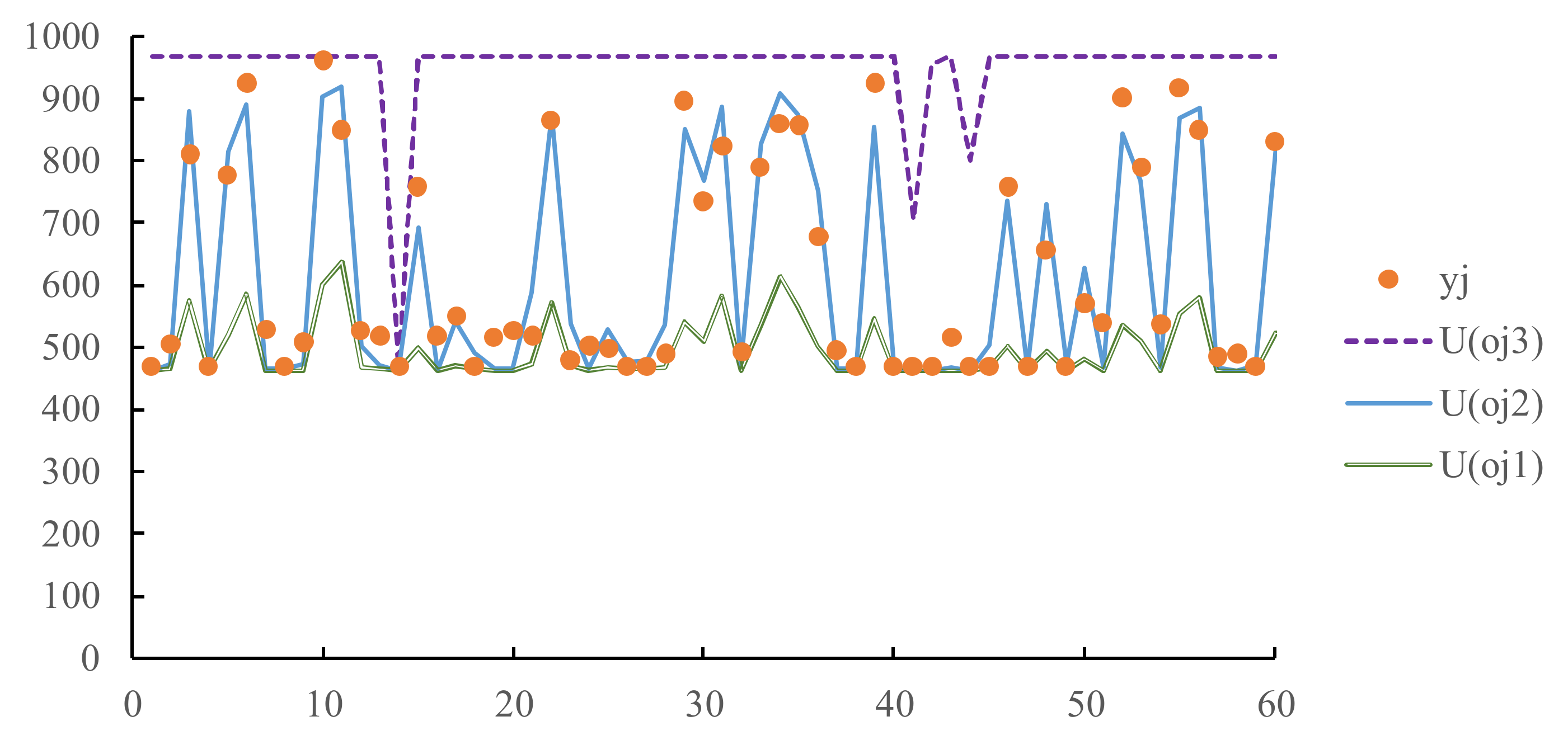
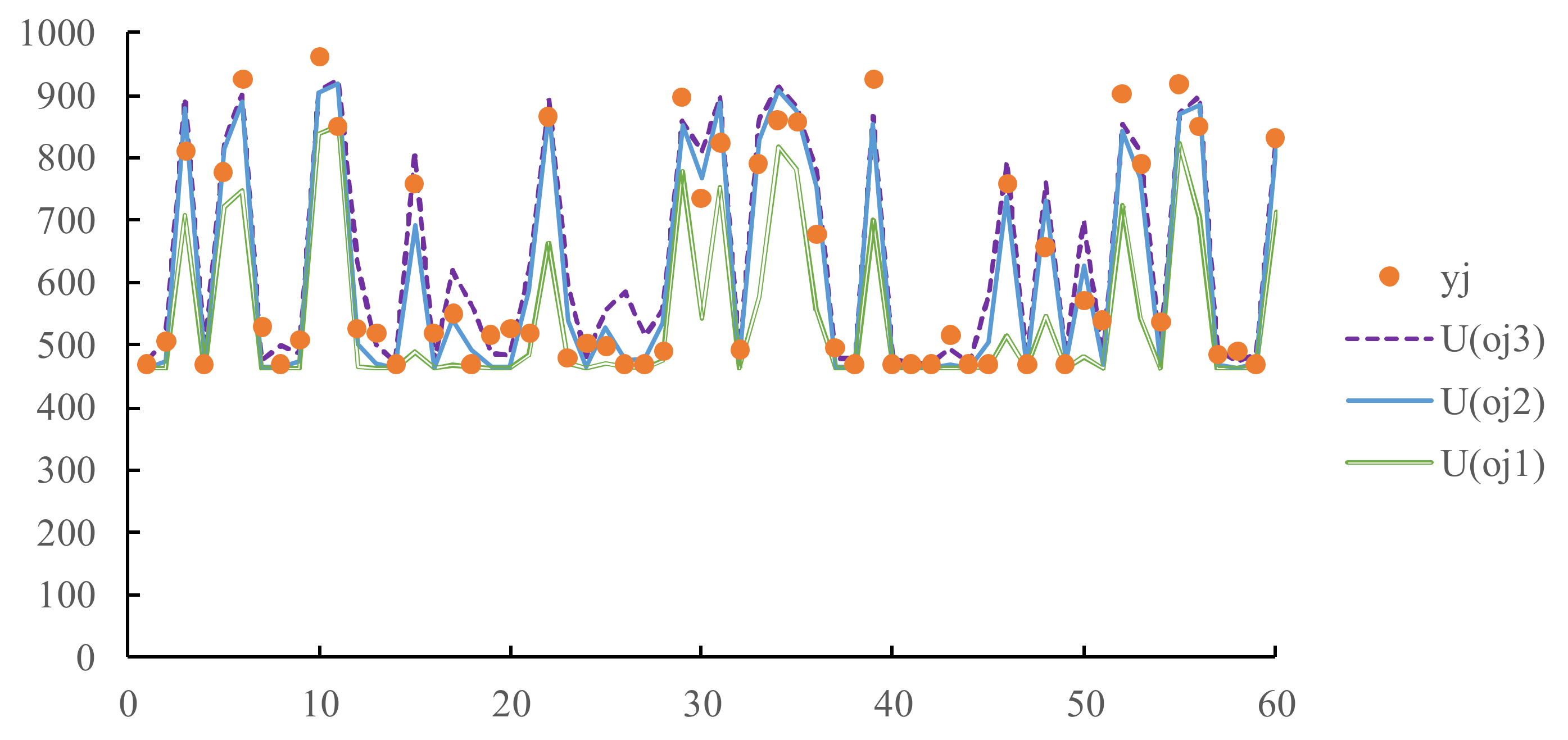
  • Fuzzifying some network parameters may not guarantee that all actual values are contained in the estimated ranges.
  • In contrast, fuzzifying a network parameter closer to the output node is more like to ensure a 100% hit rate.
  • Both the ranges estimated by fuzzifying θ o and w 1 o contain the actual value. Therefore, the fuzzy intersection (FI) of the ranges also contain the actual value, which further narrows the range of the actual value.
  • After applying the trained FFNN(3, 6, 1) to the test/unlearned data, the fore-casting precision levels achieved by fuzzifying various network parameters are evaluated and compared in Table 4. As expected, the hit rate has decreased compared to the results when applied to the training data, but is still acceptable. Fuzzifying w 1 o achieves the highest hit rate, while fuzzifying θ 1 h minimizes the average range of fuzzy forecasts.
  • The effectiveness (i.e., forecasting precision) and efficiency of the proposed methodology is compared with those of some existing methods in Table 5. All methods are implemented using MATLAB 2017a on a PC with an i7-7700 CPU of 3.6 GHz and 8 GB of RAM. Obviously, the proposed methodology maximized the hit rate for the test data without considerably widening the average range. In addition, the proposed methodology is also the most effi-cient method.

4. Conclusions and Future Research Directions

Many complex FFNNs have been constructed to improve the forecasting accuracy. Even so, a forecast is rarely equal to the actual value. In addition, the range of a fuzzy forecast generated by prevalent FFNNs does not necessarily include the actual value. In order to solve these problems, this research explores how to fuzzify the parameters of a FNN so that every fuzzy forecast generated by the FFNN contains the actual value. To achieve this goal, most previous studies have solved an NLP problem, which was computationally challenging. In contrast, this research proposes an independent fuzzification approach to fuzzify the parameters of a FNN independently. In this way, the optimal value of each fuzzy parameter can be derived theoretically, thereby enabling the construction of a precise FFNN.
After applying the proposed methodology to an illustrative case FFNN(3, 6, 1), the following conclusions are drawn:
  • Fuzzifying θ 1 h and w 11 h alone cannot guarantee that all fuzzy forecasts contain corresponding actual values.
  • Fuzzifying θ o and w 1 o has a higher chance of achieving a 100% hit rate.
  • Parameters closer to the output node have a greater impact on the forecast-ing precision, and should be fuzzified earlier.
  • Fuzzifying parameters far away from the output node cannot guarantee a 100% hit rate. Therefore, multiple such parameters should be fuzzified at the same time.
The FFNN discussed in this study is an FFNN with a single hidden layer. The pro-posed methodology can be extended to deal with a deep FFNN with multiple hidden layers [29,30,31] or recurrent layers [32]. In this case, the parameters of the output layer will be fuzzified first, then the parameters of the hidden layer closest to the output layer, and so on. In addition, FI can also be applied to aggregate the estimated ranges by fuzzifying various parameters (with 100% hit rates) to further enhance the fore-casting precision. These constitute some direction for future research.

Author Contributions

All authors equally contributed to the writing of this paper. Data curation, methodology and writing original draft: T.-C.T.C., H.-C.W. and M.-C.C.; writing—review and editing: T.-C.T.C. and H.-C.W. All authors have read and agreed to the published version of the manuscript.

Funding

This research received no external funding.

Institutional Review Board Statement

Not applicable.

Informed Consent Statement

Not applicable.

Data Availability Statement

Not applicable.

Acknowledgments

This work was supported by Ministry of Science of Technology of Taiwan.

Conflicts of Interest

The authors declare no conflict of interest.

References

  1. Ishibuchi, H.; Tanaka, H.; Okada, H. Fuzzy neural networks with fuzzy weights and fuzzy biases. In Proceedings of the IEEE International Conference on Neural Networks, San Francisco, CA, USA, 28 March–1 April 1993; pp. 1650–1655. [Google Scholar]
  2. Chen, S.X.; Gooi, H.B.; Wang, M.Q. Solar radiation forecast based on fuzzy logic and neural networks. Renew. Energy 2013, 60, 195–201. [Google Scholar] [CrossRef]
  3. Hong, Y.Y.; Chang, H.L.; Chiu, C.S. Hour-ahead wind power and speed forecasting using simultaneous perturbation stochastic approximation (SPSA) algorithm and neural network with fuzzy inputs. Energy 2010, 35, 3870–3876. [Google Scholar] [CrossRef]
  4. Kaynar, O.; Yilmaz, I.; Demirkoparan, F. Forecasting of natural gas consumption with neural network and neuro fuzzy system. Energy Educ. Sci. Technol. Part A Energy Sci. Res. 2011, 26, 221–238. [Google Scholar]
  5. De Campos Souza, P.V.; Torres, L.C.B. Regularized fuzzy neural network based on or neuron for time series forecasting. In Proceedings of the North American Fuzzy Information Processing Society Annual Conference, Fortaleza, Brazil, 4–6 July 2018; pp. 13–23. [Google Scholar]
  6. Jiang, Y.; Yang, C.; Ma, H. A review of fuzzy logic and neural network based intelligent control design for discrete-time systems. Discret. Dyn. Nat. Soc. 2016, 2016, 7217364. [Google Scholar] [CrossRef] [Green Version]
  7. De Campos Souza, P.V. Fuzzy neural networks and neuro-fuzzy networks: A review the main techniques and applications used in the literature. Appl. Soft Comput. 2020, 92, 106275. [Google Scholar] [CrossRef]
  8. Deng, Y.; Ren, Z.; Kong, Y.; Bao, F.; Dai, Q. A hierarchical fused fuzzy deep neural network for data classification. IEEE Trans. Fuzzy Syst. 2016, 25, 1006–1012. [Google Scholar] [CrossRef]
  9. Rajurkar, S.; Verma, N.K. Developing deep fuzzy network with Takagi Sugeno fuzzy inference system. In Proceedings of the 2017 IEEE International Conference on Fuzzy Systems, Naples, Italy, 9–12 July 2017; pp. 1–6. [Google Scholar]
  10. Mudiyanselage, T.K.B.; Xiao, X.; Zhang, Y.; Pan, Y. Deep fuzzy neural networks for biomarker selection for accurate cancer detection. IEEE Trans. Fuzzy Syst. 2019, 28, 3219–3228. [Google Scholar] [CrossRef]
  11. Liang, X.; Wang, G.; Min, M.R.; Qi, Y.; Han, Z. A deep spatio-temporal fuzzy neural network for passenger demand prediction. In Proceedings of the 2019 SIAM International Conference on Data Mining, Calgary, AB, Canada, 2–4 May 2019; pp. 100–108. [Google Scholar]
  12. Qasem, S.N.; Mohammadzadeh, A. A deep learned type-2 fuzzy neural network: Singular value decomposition approach. Appl. Soft Comput. 2021, 105, 107244. [Google Scholar] [CrossRef]
  13. Radulović, J.; Ranković, V. Feedforward neural network and adaptive network-based fuzzy inference system in study of power lines. Expert Syst. Appl. 2010, 37, 165–170. [Google Scholar] [CrossRef]
  14. Hou, Y.; Zhao, L.; Lu, H. Fuzzy neural network optimization and network traffic forecasting based on improved differential evolution. Future Gener. Comput. Syst. 2018, 81, 425–432. [Google Scholar]
  15. Sharifian, A.; Ghadi, M.J.; Ghavidel, S.; Li, L.; Zhang, J. A new method based on Type-2 fuzzy neural network for accurate wind power forecasting under uncertain data. Renew. Energy 2018, 120, 220–230. [Google Scholar]
  16. Wen, Z.; Xie, L.; Fan, Q.; Feng, H. Long term electric load forecasting based on TS-type recurrent fuzzy neural network model. Electr. Power Syst. Res. 2020, 179, 106106. [Google Scholar]
  17. Chen, T.; Wu, H.C. A new cloud computing method for establishing asymmetric cycle time intervals in a wafer fabrication factory. J. Intell. Manuf. 2017, 28, 1095–1107. [Google Scholar] [CrossRef] [Green Version]
  18. Chen, T.C.; Lin, Y.C. A collaborative fuzzy-neural approach for internal due date assignment in a wafer fabrication plant. Int. J. Innov. Comput. Inf. Control. 2011, 7, 5193–5210. [Google Scholar]
  19. Chen, T.C.T.; Honda, K. Fuzzy Collaborative Forecasting and Clustering: Methodology, System Architecture, and Applications; Springer International Publishing: Cham, Switzerland, 2020. [Google Scholar]
  20. Chen, T.; Wang, Y.C. Incorporating the FCM–BPN approach with nonlinear programming for internal due date assignment in a wafer fabrication plant. Robot. Comput. Integr. Manuf. 2010, 26, 83–91. [Google Scholar] [CrossRef]
  21. Tarray, T.A.; Bhat, M.R. A nonlinear programming problem using branch and bound method. Investig. Oper. 2018, 38, 291–298. [Google Scholar]
  22. Chen, T. An effective fuzzy collaborative forecasting approach for predicting the job cycle time in wafer fabrication. Comput. Ind. Eng. 2013, 66, 834–848. [Google Scholar] [CrossRef]
  23. Chen, T. An efficient and effective fuzzy collaborative intelligence approach for cycle time estimation in wafer fabrication. Int. J. Intell. Syst. 2012, 30, 620–650. [Google Scholar] [CrossRef]
  24. Wang, Y.C.; Tsai, H.R.; Chen, T. A selectively fuzzified back propagation network approach for precisely estimating the cycle time range in wafer fabrication. Mathematics 2021, 9, 1430. [Google Scholar] [CrossRef]
  25. Nocedal, J.; Wright, S. Numerical Optimization, 2nd ed.; Springer Science & Business Media: Berlin/Heidelberg, Germany, 2006. [Google Scholar]
  26. Ramchoun, H.; Idrissi, M.A.J.; Ghanou, Y.; Ettaouil, M. Multilayer perceptron: Architecture optimization and training. Int. J. Interact. Multim. Artif. Intell. 2016, 4, 26–30. [Google Scholar]
  27. Cilimkovic, M. Neural networks and back propagation algorithm; Institute of Technology Blanchardstown: Dublin, Ireland, 2015; Volume 15, pp. 1–12. [Google Scholar]
  28. Lin, Y.C.; Chen, T. An advanced fuzzy collaborative intelligence approach for fitting the uncertain unit cost learning process. Complex Intell. Syst. 2019, 5, 303–313. [Google Scholar]
  29. Karsoliya, S. Approximating number of hidden layer neurons in multiple hidden layer BPNN architecture. Int. J. Eng. Trends Technol. 2012, 3, 714–717. [Google Scholar]
  30. Moghaddam, A.H.; Moghaddam, M.H.; Esfandyari, M. Stock market index prediction using artificial neural network. J. Econ. Financ. Adm. Sci. 2016, 21, 89–93. [Google Scholar]
  31. Jana, G.C.; Swetapadma, A.; Pattnaik, P.K. Enhancing the performance of motor imagery classification to design a robust brain computer interface using feed forward back-propagation neural network. Ain Shams Eng. J. 2018, 9, 2871–2878. [Google Scholar]
  32. Šestanović, T.; Arnerić, J. Can recurrent neural networks predict inflation in Euro Zone as good as professional forecasters? Mathematics 2021, 9, 2486. [Google Scholar]
Figure 1. Crisp forecasts based on the cores of fuzzy parameters.
Axioms 10 00282 g001
Figure 2. Estimated ranges by fuzzifying θ o .
Axioms 10 00282 g002
Figure 3. Ranges estimated by fuzzifying w 1 o .
Axioms 10 00282 g003
Figure 4. Estimated ranges after fuzzifying θ 1 h .
Axioms 10 00282 g004
Figure 5. Ranges of actual values estimated by fuzzifying w 11 h .
Axioms 10 00282 g005
Table 1. Collected data.
j x j 1 x j 2 x j 3 y j
1265302028468
2224402018507
3173522641811
4151361837468
5322552274776
6167562508926
90311392170468
Min125291173463
Max364573269967
Table 2. Normalized data.
j z j 1 z j 2 z j 3 a j
10.5850.0360.4080.010
20.4150.3920.4030.087
30.1990.8350.7000.691
40.1110.2670.3170.010
50.8250.9420.5250.621
60.1740.9620.6370.919
900.7800.3400.4760.010
Table 3. Optimized cores of fuzzy parameters.
w 112 h * w 122 h * w 132 h * w 142 h * w 152 h * w 162 h * w 212 h * w 222 h * w 232 h * w 242 h *
2.0343.410−0.349−2.615−2.5571.2133.912−1.7461.8133.187
w 252 h * w 262 h * w 312 h * w 322 h * w 332 h * w 342 h * w 352 h * w 362 h * θ 12 h * θ 22 h *
−2.0903.0823.733−0.4243.9643.831−4.7544.9113.2225.251
θ 32 h * θ 42 h * θ 52 h * θ 62 h * w 12 o * w 22 o * w 32 o * w 42 o * w 52 o * w 62 o *
9.1832.2932.5694.7854.8444.740−2.6413.727−4.9053.668
θ 2 o *
9.475
Table 4. Forecasting precision levels achieved by fuzzifying various network parameters.
Fuzzifying   θ o Fuzzifying   w 1 o Fuzzifying   θ 1 h Fuzzifying   w 11 h
Hit Rate97%100%63%63%
Average Range367.3457.9122.7228.5
Table 5. Comparing the effectiveness and efficiency of the proposed methodology with those of existing methods.
MethodHit RateAverage RangeExecution Time (sec)
FFNN-NLP [18]82%407168
FFNN-GP [20]76%48246
FFNN (only θ ˜ o fuzzified) [22]97%367<1
The proposed methodology w 1 o fuzzified)100%458<1
Publisher’s Note: MDPI stays neutral with regard to jurisdictional claims in published maps and institutional affiliations.

