Application of Data Analytics Techniques to Establish Geometallurgical Relationships to Bond Work Index at the Paracutu Mine, Minas Gerais, Brazil

Abstract

Analysis of geometallurgical data is essential to building geometallurgical models that capture physical variability in the orebody and can be used for the optimization of mine planning and the prediction of milling circuit performance. However, multivariate complexity and compositional data constraints can make this analysis challenging. This study applies unsupervised and supervised learning to establish relationships between the Bond ball mill work index (BWI) and geomechanical, geophysical and geochemical variables for the Paracatu gold orebody. The regolith and fresh rock geometallurgical domains are established from two cluster sets resulting from K-means clustering of the first three principal component (PC) scores of isometric log-ratio (ilr) coordinates of geochemical data and standardized BWI, geomechanical and geophysical data. The first PC is attributed to weathering and reveals a strong relationship between BWI and rock strength and fracture intensity in the regolith. Random forest (RF) classification of BWI in the fresh rock identifies the greater importance of geochemical ilr balances relative to geomechanical and geophysical variables.

1. Introduction

A geometallurgical relationship intrinsically links rock properties—i.e., mineralogy, texture, geochemistry and physio-mechanical properties—to its processing behavior. Understanding these relationships is key to building 3D spatial models that relate mineral processing performance to the physical variability in an orebody [1]. Geometallurgical data include measures of processing performance indicators and information on the orebody characteristics that can potentially be linked to these indicators. Such information can include multielement geochemistry, geomechanical parameters and petrophysical properties [2]. Analysis of geometallurgical data is an essential basis for establishing geometallurgical relationships, but this can be challenging given complex multivariate relationships in the datasets and omnipresent spatial variability within an orebody [3,4]. Complex multivariate relationships can be a product of geometallurgical variable interactions, non-normal underlying data distributions or non-linear functions of the processing performance variable. Adding to the complexity is the uncertainty of knowing, a priori, the number of domains that adequately describe the spatial and physical variability of an orebody [5]. Geometallurgical data analysis may fail to filter out or capture hidden data structures that result from the physical variability in the orebody on different scales. These data structures can also occlude underlying geometallurgical relationships. Challenges also include non-additive geometallurgical variables, for example, comminution indices; variables with different measurement units; and datasets with variables belonging to different sample spaces, such as compositional and non-compositional data [4,6,7,8,9]. A proper geometallurgical data analysis must account for all of these data complexities to be effective in establishing geometallurgical relationships.

Data analytics techniques—that is, unsupervised and supervised learning—encompass both multivariate statistical methods and information science algorithms that are useful for geometallurgical study [10,11,12] because they help to establish orebody domains and variable associations meaningful for geometallurgical relationships. Unsupervised learning refers to techniques which identify the presence or lack of relationships and patterns in multivariate data without prior knowledge of an output variable. Supervised learning are methods that predict or classify observations using prior knowledge obtained from an output variable by fitting (“learning”) functions from predictor input variables. Principal component analysis (PCA) is an unsupervised technique generally used for dimensional reduction, decorrelation and identifying associations of geometallurgical variables and delineating classes [5,6,13,14,15]. Cluster analysis, such as K-means, is another unsupervised technique that has been employed to explore similarities and groupings of geometallurgical data [16,17]. Cluster analysis can be also used for geometallurgical domaining by spatially analyzing clustering results in relation to orebody characteristics. The random forest (RF) is a supervised method that is suitable for approximating non-linear functions and accommodating high-order variable interactions [18,19]. While RF has been primarily used in geometallurgy for prediction [20,21,22], the model results show which input variables have the most predictive importance for each predicted class. In this regard, RF is useful for studying geometallurgical relationships for different orebody domains.

The Paracatu orebody is hosted within a relatively homogenous succession of black phyllites. Deep lateritic weathering has introduced significant geological variability to the ore body. These characteristics offer a unique opportunity to investigate the application of data analytics to identify key geometallurgical relationships that can be linked to the geological attributes of the deposit. Accordingly, this study presents a systematic analytical workflow to identify geometallurgical relationships to Bond ball mill work index (BWI) at the Paracatu mine. The geometallurgical dataset used included geomechanical, geophysical and multielement geochemical data obtained from drillcore samples. Compositional representations are applied to remove constraints from the compositional multielement geochemical data. The multivariate data is simplified using PCA and associations amongst geometallurgical variables are explored in relation to BWI. Geometallurgical relationships are also studied using RF classification of BWI. K-means cluster analysis is used to group PCA results and clusters are spatially visualized to understand relationships to the weathering profile and structure of the orebody.

2. Paracatu Mine

Paracatu Mine, operated by Kinross Gold, is a large open-pit gold operation located in Minas Gerais state in Brazil, approximately 230 km southeast of Brasilia. The operation is currently the largest gold producer in Brazil with proven and probable mineral reserves of an estimated 7.9 Moz. gold at an average grade of 0.4 g/t [23].

The Paracatu mineral deposit is stratigraphically located in the Morro Do Ouro member of the Paracatu Formation (Figure 1). The deposit is structurally situated on the hanging wall of a thrust fault within a regional East verging fold-thrust belt system [24,25]. The Paracatu orebody is a kilometer-scale structure that is oriented sub-parallel to the stratigraphy, defining a tabular lens-shaped structure striking north-north-west (NNW) and moderately dipping towards the south-west (SW) [26] (Figure 2 and Figure 3). The orebody is 5 km long, 2 km wide and up to 140 m thick.

The Paracatu gold deposit is hosted in weakly sericitized and chloritized carbonaceous black phyllite. The sedimentary protolith represents a relatively homogenous lithology composed of deformed carbonaceous siltstones and shales metamorphosed to lower greenschist facies. Common metamorphic mineral assemblages at Paracatu include sericite, quartz, ilmenite, plagioclase, trace carbonates and sulfides [26]. Weak carbonate alteration is dominated by siderite, dolomite and ankerite assemblages [28,29]. Sulfide mineralization includes arsenopyrite, pyrite, pyrrhotite and traces of sphalerite, galena and chalcopyrite. The fabric of the mineralized phyllite is dominated by shear-related structures such as tight asymmetric folding, rootless folds, sigmoidal boudins and rare slickensides (Figure 4). In contrast, non-mineralized phyllites contain fewer boudins, less carbonates and sulfides and greater content of chlorite relative to the mineralized counterparts. Bedding is relatively well preserved in low-strain zones, where it is subparallel to the main foliation. However, strong structural transposition in high-strain zones makes it difficult to recognize primary sedimentary features [26]. The mineralized and non-mineralized phyllites are also differentiated by geochemical signature. The mineralized zone is enriched in Au, Ag, As, Pb, Zn, C and S, while the non-mineralized zone contains higher proportions of Zr, V, Cr and Al [30].

The Paracatu orebody underwent intense lateritic weathering; which has formed a regolith profile 20–80 m thick, Figure 5 and Figure 6. From top to bottom, the regolith includes well-developed red lateritic saprolite; in which the primary rock fabrics have been completely obliterated. The saprolite gradually transitions into saprock where the black color and primary fabrics of the phyllites are preserved but the lithological competence is significantly reduced relative to the unweathered counterparts. The saprock transitions downwards into hard bedrock, which is composed of competent unweathered black phyllite.

Weathering has strong control of grindability and throughput at Paracatu [14]. Therefore, for operational purposes the orebody has been subdivided into an upper oxidized B1 ore, in the mine terminology, that represents mineralized saprolite and saprock and a stratigraphically lower B2 ore, that correlates with mineralized fresh bedrock. The thicknesses of the oxidized B1 ore is approximately 20 to 80 m, with substantial lateral variability across the mine.

Operationally, the Paracatu mine is a conventional shovel-and-truck operation with two comminution plants. Plant 1 includes primary and secondary crusher in circuit with ball mills for grinding to 80% passing 150 microns. The BWI near surface, dominated by B1 ore, is generally less than 7 kWh/t [28]. The BWI increases with depth to 19 kWh/t in the domain correlating with B2 ore. The softer B1 ore has been substantially mined out. Progression of mining into the deeper and harder B2 ore necessitated the installation of Plant 2 in 2008 to meet throughput requirements. This plant contains an in-pit MMD crusher and a SAG mill in circuit with four ball mills and has a nominal plant capacity of 41 Mt/a for a Bond work index (BWI) below 8.7 kilowatt hours per ton (kWh/t). A study by [29] used the B1 and B2 ore as a basis to establish geometallurgical domains for gold recovery and flotation properties. However, while BWI was incorporated as a predictor variable, the study determined no significant geometallurgical relationships to grindability. Thus, use of these domains to characterize BWI spatial variability is inappropriate. This study is motivated by an operational need to understand geometallurgical relationships to grindability, especially in the highly variable B2 ore.

3. Analytical Procedure

In this study, data pre-processing was conducted in Microsoft Excel. The R programming language [31] and the R Studio statistical computing environment was used for tasks in geochemical data imputation, compositional data analysis and data analytics.

3.1. Data Collection and Pre-Processing

Data on the Paracatu orebody is available from mineral exploration and mine operational drilling and sampling programs from 1993 to 2016. The majority of data was collected after Kinross acquired Paracatu in 2003. The dataset used in this study includes (1) Bond ball mill work index (BWI); (2) point load strength index (PLSI) and (3) rock quality designation (RQD) as two geomechanical variables; (3) magnetic susceptibility (MAGSUSC), a geophysical variable; and (4) multielement geochemical data.

Table 1. Summary of the geometallurgical dataset in this study. Downhole interval of representation signifies the stepwise drillhole interval for which the variable was available in the Paracatu database.

Geometallurgical Variable	Units	Number of Records	Downhole Interval of Representation	Min	25th Percentile	Median	75th Percentile	Max	Mean	Std. Dev.
Axial point load strength index (PLSI_AX)	MPa 1	945	4 m	0.1	3.9	7.5	9.4	16.7	6.8	3.5
Rock quality designation (RQD)	%	796	Ranges from 1 to 3 m	0	81	94	99	100	84	24
Magnetic susceptibility (MAGSUSC)	Unitless	3562	1 m	0.01	0.32	0.72	1.41	7.5	0.96	0.84
Multielement geochemistry	% 2; ppm 3	3562	1 m	See Table 2.
Bond ball mill work index (BWI)	kWh/t 4	977	Ranges from 6 m to 12 m	2.0	12.0	14.1	15.4	23.1	13.1	3.5

¹ Mega Pascals. ² Percentage composition. ³ Parts per million. ⁴ Kilowatt hours per ton.

presents a statistical summary of the dataset and downhole interval of representation for each variable.

The BWI is obtained from the Bond ball mill test, a locked-cycle laboratory test that measures the ball mill grinding energy required for a given throughput of ore. It indicates ore resistance and breakage characteristics on the micron-scale. BWI tests are conducted at the Paracatu mine laboratory using a standard Bond ball mill and test methodology. The feed is prepared by compositing fractions of one-meter core segments from the sample interval after initial crushing to 2 mm [28]. The composite feed is then ground to 80 % passing product size of 150 microns.

The point load strength index (PLSI) is obtained from the point load test, a portable geomechanical test in which a drillcore sample is point loaded via two opposing steel plates and compressed until breakage. The PLSI is widely used as an estimate of the rock strength of drillcore in geotechnical logging. In the presence of foliation, the test can be conducted in a diametral or an axial orientation, relative to the drillcore axis, to accommodate any anisotropic influence on rock strength. The point load test is routinely conducted at Paracatu in both orientations to account for the phyllite foliation. Axial tests at Paracatu are generally perpendicular or at high angles to the shallow dipping foliation. This test configuration generally produces a PLSI that is more representative of the rock matrix strength, compared with those tests performed subparallel to the foliation planes, that commonly result in lower PLSI due to failure along foliation planes. The PLSI has been shown to correlate with comminution indices when scale-effects are properly accounted for [32]. A study by [33] determined a strong correlation between axial PLSI and ore breakage parameters determined from the drop weight test. In this study, only axial PLSI values (PLSI_AX) were retained for subsequent analysis.

Rock quality designation (RQD) is a geotechnical parameter that characterizes the intensity of natural discontinuities in drillcore. It represents the percentage of core pieces greater than 10 cm in length within a given core interval. The RQD is typically recorded every meter or for every core run interval, which is the length of core recovered from a single drilling core barrel. RQD is routinely measured at Paracatu and is recorded in intervals varying from 1 m to 3 m. RQD has been correlated to comminution indices because it can capture ore competency [34]. However, this can be influenced by scale-effects. For example, if RQD is high, indicative of widely spaced jointing, then it may be inappropriate to use it to explain the variability in ore breakage below the centimeter or meter scale.

Magnetic susceptibility is a geophysical property that measures the degree of magnetism of a material. It is generally used to detect magnetic minerals in mineral exploration. MAGSUSC at Paracatu is recorded to detect pyrrhotite-rich zones. Measurements are recorded at 1 m intervals and represent the average of ten measurements taken within the interval using a handheld KT-10 magnetic susceptibility meter [29]. Petrophysical characteristics such as magnetism have demonstrated correlation to ore breakage, although these associations depend on the mineral deposit type and associated mineralogy [35].

The multielement geochemical data were analyzed in drill core samples collected every meter. The geochemical dataset consists of 39 elements including Au, Li, Na, Ag, Bi, Sb, Fe, Pb, As, Sr, Cd, Ba, Zn, Sn, Mo, Mn, Be, Sc, Cu, W, K, Ti, S, P, Co, Ni, Th, Mg, Al, Se, Zr, V, U, B, Cr, Ca, Y, La and Tl. The majority of the multielement geochemical data was analyzed at SGS Brazil, Method GE-ICP14B, using a room temperature aqua regia digestion and elemental determination through inductively coupled plasma atomic emission spectrometry (ICP-AES). It is noteworthy that aqua regia is a partial digestion and consequently the elemental abundances are lower than the actual concentrations in the digested rocks. Silicate-hosted trace elements Ti, Th, Zr, La, Sc, V, Sr, Ba, Be, W, U, Pb and Tl and major elements Na, K and Al are commonly underreported in aqua regia digestions. In contrast, sulfide- and oxide-hosted trace elements Ag, Bi, Sb, As, Cd, Cu and Zn are near-totally to totally digested in the aqua regia. Conventional geochemical analysis that requires stoichiometric relationships are not applicable to an aqua regia digestion due to incomplete digestion. However, given that the aqua regia digestion is matrix dependent, different rock types digest differently, a data analytics approach is amenable to investigate this type of geochemical data because the focus is on pattern recognition and function fitting in which a total digestion is not required [36].

Gold was analyzed primarily at the mine lab by fire assay and atomic absorption spectroscopy (AAS) on 50 g pulps. Multielement geochemistry has been used to model comminution parameters [37,38]. The data can indicate compositional variations associated with changes in geochemistry and mineralogy, which may be useful to distinguish different materials with distinct breakage characteristics. The multielement was pre-processed to select a subcomposition of geochemical elements that are most informative of geochemical signatures associated with mineralization and lithology. To do so, the elements with >50% of measurements below laboratory detection limit were removed from the dataset [39]: Li, Na, Ag, Bi, Sb, Cd, Sn, Mo, Sc, W, Ti, Th, Be, Se, V, B, Y, La and Tl. Histograms of the remaining elements were studied to select those having an appropriate granularity and availability of data within the detection range. Finally, these elements were cross-referenced with those established from geochemical studies at Paracatu [26,30]. After pre-processing a 20-element subcomposition of geochemical variables was retained for data analysis (

Table 2. Summary of 20-element subcomposition selected as geochemical variables for this study.

Geochemical Element	Unit	LDL 1	Mean	Std. Dev.	Min	25th Percentile	Median	75th Percentile	Max
Fe	%	0.01	4.25	0.93	0.01	3.9	4.3	4.7	15
Pb	ppm	3	54	115	3	13	23	48	1987
As	ppm	5	1537	1735	5	401	995	1995	10,616
Sr	ppm	1	22	22	1	17	22	28	1143
Ba	ppm	1	30	10	1	23	28	35	149
Zn	ppm	1	98	103	1	59	80	103	1818
Mn	%	0.01	0.05	0.02	0.01	0.04	0.05	0.06	0.16
Au	ppm	0.002 2	0.33	0.34	0.001	0.11	0.25	0.44	6.75
Cu	ppm	1	39	20	1	31	37	45	930
K	%	0.01	0.21	0.06	0.01	0.16	0.2	0.24	0.62
S	%	0.01	0.89	0.42	0.01	0.59	0.88	1.18	2.38
P	%	0.01	0.06	0.02	0.01	0.04	0.06	0.07	0.2
Co	ppm	3	16	5	3	13	15	18	90
Ni	ppm	1	29	13	1	26	29	32	191
Mg	%	0.01	0.55	0.37	0.01	0.47	0.55	0.64	12.5
Al	%	0.01	0.88	0.64	0.01	0.39	0.68	1.20	4.40
Zr	ppm	1	10.07	4.16	1	7.3	9.6	12	32
Ca	%	0.01	0.37	0.46	0.01	0.25	0.36	0.46	15
V	ppm	3	9	7	3	4	6	10	77
Cr	ppm	1	8	11	1	3	4	11	159

¹ Lower detection limit, which represents the lowest quantity of a given element that can be detected by the ICP-OES package. ² LDL of Au represents that of the AAS method.

). The unsupervised statistical techniques require a complete data matrix. Therefore, the data were cleaned by checking observations with erroneous values and removing those missing data for BWI, PLSI_AX and RQD. The non-detect properties were considered for each geochemical variable. Left-censored and right-censored values are those which are below and above the laboratory detection limits, respectively. All 20 geochemical variables have only left-censored values which are reported as each variable’s LDL. In addition, most variables have a right-skewed statistical distribution, typical of geochemical variables [40]. Data imputation is typically required for non-detect values since their presence can complicate multivariate analysis [38]. Here, non-detects are imputed by the multiplicative lognormal replacement method using the R package ‘zCompositions,’ after the conversion of all units to ppm [41,42,43]. This imputation method is appropriate for the geochemical data because it accommodates its compositional data form, does not assume multivariate normality and is appropriate for positive data with right-skewed distributions [39,40,41].

In legacy geometallurgical datasets the tests are commonly collected in independent sampling campaigns using different sampling intervals. A necessary pre-processing step needs to address the problem of unequal drillcore intervals over which different variables are represented. One option is to match variables represented over a shorter interval to those represented over longer intervals by using some form of compositing. These resolutions are used in geostatistics, where the goal is to reduce erratic variation in short distances and reduce the amount of data for 3D spatial modelling. However, they are unsuitable when attempting to explore geometallurgical relationships because they may not suit variable constraints, for example, non-additivity or make inferences and parametric assumptions about the variables that mask their true variability. Granularity of variables represented over shorter intervals may also be reduced. This study uses a repetition strategy that downscales the intervals of all variables to the shortest interval of 1 m, which preserves data resolution and respects non-additivity properties. Variables represented over longer intervals were discretized into 1 m intervals and their values were repeated. Since BWI has the largest drillcore interval of representation, 6 to 12 m, a unique identifier was created for each BWI sample using the drillhole ID and interval endpoints. Other variables were collocated with the BWI using this identifier. In the processed dataset BWI, PLSI_AX and RQD were replicated to match the MAGSUSC and geochemical variables, collected at the shortest interval of 1 m, for each meter represented by the BWI sample. A dataset of n = 3596 observations and m = 24 variables was obtained using these pre-processing techniques.

The following terminology is used for this study. Orebody variables refer to the PLSI_AX, RQD, MAGSUSC and geochemical variables, all of which are used as predictors for the processing variable BWI. Geochemical variables refer to those engineered by compositional data analysis of the 20-element subcomposition. The regolith is the weathered zone of the Paracatu orebody containing the saprolite and saprock layers. The fresh rock refers to the fresh intact phyllite bedrock. Observations are records in the dataset which have downscaled values for PLSI_AX, RQD and BWI and are represented every meter. BWI samples or sample groups refer to the original composited BWI sample represented over the 6 to 12 m interval.

3.2. Compositional Data Analysis

Multielement geochemical data is a type of compositional data and the constraints related to its compositional properties have been documented in geometallurgical studies [3,4,8,13]. Compositional data is a special form of data that is non-negative, carries information in the ratios of its variables and sums to some constant [44]. Therefore, compositional data exists in a constrained space, rendering it unsuitable for direct application of statistical techniques; which are mostly developed for unconstrained mathematical spaces [45]. To accommodate the special properties of compositional data different compositional representations have been proposed including the additive log-ratio (alr), centered log-ratio (clr) and isometric log-ratio (ilr) [44,45,46]. These representations project compositional data into the Euclidean real space and can be used for statistical analysis.

The dataset used in this study include compositional data and non-compositional data, such as BWI, PLSI_AX, RQD and MAGSUSC. This requires an analytical approach that accommodates the special properties of compositional data in the presence of external variables [8]. This is important when applying PCA for decorrelating effects and for studying relationships between compositional and non-compositional data [47]. For this analysis, the geochemical elements, are the compositional parts of the 20-part subcomposition. In geochemistry, a common practice is grouping chemical elements into composite variables, the relative ratios of which can represent potential associations with lithogeochemical domains [39,48].

The variation matrix, the variance of the log-ratios between variables [44], is calculated for the 20-element geochemical subcomposition and used as a dissimilarity measurement for hierarchical cluster analysis to investigate relationships between elements [39,44,49]. The aR pckage ‘rgr’ is used to compute the variation matrix [50] and the hierarchical cluster dendrogram is generated with the R package ‘dendextend’ [51,52]. To reduce dimensionality and redundancy between correlated variables, composite variables are defined by the groupings of elements on the indicated in the cluster dendrogram [39,53]. The new matrix of composite geochemical variables is centered geometric mean for consistency with the algebraic geometry of compositions [46]. These methods were executed using the R package ‘compositions’ [54,55]. In addition, balances (ilr coordinates) and clr coefficients of the composite variables were determined using the R package ‘robCompositions’ [56,57]. The ilr variables are determined using the sequential binary partition [46] suggested by the variation matrix cluster dendrogram [39,53]. In this study, the term ilr variables is interchangeable with balances and il coordinates. Use of ilr variables as a substitute for raw compositional data in supervised learning may be appropriate because both can show comparable results [53]; ilr variables also offer the advantage of capturing relative information between elements and element groups.

3.3. Unsupervised Learning

Principal component analysis (PCA) and K-means cluster analysis are integrated to establish significant geometallurgical groupings in the Paracatu orebody.

PCA is an unsupervised method used for reducing multivariate dimensionality to filter noise and decorrelating redundant variables. PCA can reveal hidden data structures and allows exploration of significant associations amongst variables. To achieve this, the original observations are mapped to a reduced dimensional space via an orthogonal transformation [58,59,60]. Principal components are the new set of variables calculated from linear combinations of the original variables. A biplot is used for graphical representation of the reduced principal component space defined by the principal components selected for visualization. The axes of the biplot are the principal components selected for visualization. Variables and observations are represented in the biplot, respectively, as vectors (loadings) and coordinates (scores). Provided that the selected principal components (PCs) capture a relatively large proportion of the variance, the biplot can provide insight into the original multivariate data structure [61].

The presence of both compositional and non-compositional data in the data matrix complicates PCA due to differences in the sample space of these datasets. However, the issue can be accommodated by using balances of the compositional data [47]. Prior to data analysis, the non-compositional variables BWI, PLSI_AX, RQD and MAGSUSC are standardized to their z-scores, by subtracting the means and dividing by the standard deviation of the variables. Accordingly, the new data matrix for PCA includes balances of the geochemical data and standardized non-compositional variables. PCA is applied via singular value decomposition (SVD). To construct a biplot, the loadings and scores of the ilr-coordinates are converted to clr coordinates and the PCA results of the non-compositional results are then incorporated. The resulting biplot of compositional and non-compositional variables [47] has graphical characteristics for which the interpretation of angles between compositional and non-compositional loading vectors is similar to that of the standard biplot. This method is used in this study to integrate compositional and non-compositional data for PCA analysis using R package ‘robCompositions’ [56,57]. Scree plots of the cumulative percentage of variance explained by the PCs are used to define the number of significant PCs to retain for further analysis. The significance of the PCs is evaluated against the Paracatu orebody characteristics. The scree plot is also used as a tool to understand if there are limitations of PCA associated with the complex characteristics of geometallurgical data. Lack of a significant inflection point within the first few PCs and similarities amongst their variance proportions may imply that the data does not have significant structure in terms of variability. It could also indicate that the linear dimensionality reduction of PCA cannot capture complex multivariate distributions [3].

K-means cluster analysis is an algorithm that establishes groupings in the data structure using the squared Euclidean distance between observations as a measure of dissimilarity [62,63,64]. Data clustering cannot begin without defining a desired number of K-clusters. A conventional method of selecting K is to parametrically vary it and study the difference in within-cluster sum squared errors. A plot of these results can indicate an inflection point at a K value for which significant minimization of cluster variance is achieved. This number of K-clusters is then chosen and interpreted for its significance. An uncertainty will still exist in whether the clusters are forming meaningful groupings or clustering noise in the data [65]. Therefore, the number of K optimum clusters can only be estimated when domain knowledge is integrated into the interpretation of the clusters [39]. Another important consideration is the configuration of initial cluster centroids. Although randomly placed, a bias in their configuration relative to the data structure can lead to convergence to a suboptimal local minimum for the error function [64]. Here, we apply K-means following the algorithm variation of [63]. In this approach, several different random configurations of the initial cluster centroids are specified. Then, K-means is performed for each configuration and results are reported for the configuration that best minimizes the error function.

Combining cluster analysis and PCA by clustering PCA results is a common technique for unsupervised identification of domains in geosciences [48]. In this study, K-means is used to cluster the PC scores using the R function ‘kmeans’ [31]. The results of cluster analysis are used to create a categorical variable whose labels represent the cluster membership of each observation. K number of clusters are established by analyzing the cluster variances resulting from K ranging between 1 and 10. Twenty different random configurations were specified for each K to account for any bias in centroid position during clustering initialization. PCA biplots and K-means plots are created using the R packages ‘factoextra’ [66], ‘ggplot2’ [67,68] and ‘ggsci’ [69]. The resulting clusters are interpreted for significance using knowledge of the Paracatu orebody. The PCA clusters are visualized in 3D geological space to evaluate their spatial relationship to the Paracatu orebody weathering profile and structure, using GEOVIA GEMS (Version 6.8.2.1) software by Dassault Systemes.

3.4. Supervised Learning with Random Forests

In this study, random forest (RF) is used for supervised learning to obtain variable importances. RF is an ensemble method that uses a multitude of decision trees for prediction by incorporating bootstrap aggregation and randomized selection of a subset of predictors [18,70]. A set of equally sized bootstrap samples are independently drawn from the training set. Each sample is used to train a single tree. During the tree training, the tree is limited to information from a randomly selected subset of predictor variables for each internal node split. A portion of the bootstrap sample, the out-of-bag (OOB), is held out during the training of the tree. After training, the OOB sample is used to cross-validate the tree and yields an OOB accuracy. A new observation is predicted by having every tree classify a response using the predictor values and then taking the consensus response over all trees to be the predicted class. Variable importance is determined using the OOB sample before any prediction on test observations. Once the OOB accuracy is determined, the values of a single predictor variable are randomly permuted within the OOB sample. Then, the modified OOB sample is classified with the tree and yields a permutation accuracy. The difference between the true OOB accuracy and the OOB permutation accuracy of the tree yield the variable importance for the permuted predictor. This process is repeated for all variables in the OOB sample to produce a set of variable importance scores, expressed as mean decrease in accuracy, for each tree. A raw variable importance score is obtained by averaging set of scores over all trees. Variable importance provides a descriptive assessment and ranking of the significance of a given predictor in the performance of the RF model.

RF is used for supervised classification of BWI. This requires class definition of BWI ranges that represent changes in ore grindability. In this study, the BWI classes are defined by K-means clustering of the BWI sample data for K = 4,3 and 2 clusters. A corresponding number of K quantiles are assigned as seeds for the initial cluster centroids. The resulting cluster boundaries establish a range of BWI in each class. Selection of K for the number of classes requires the consideration of class imbalance [53], which refers to how many observations belong to one class relative to another. Highly imbalanced classes can be detrimental to supervised learning because the model is trained on different class proportions and consequently overfit to better represented classes. To alleviate the effect of class imbalance, the K BWI clusters are selected which have relatively similar proportions and a suitable within-cluster sum of squared error. Then, the cluster boundaries are assessed against the operational BWI boundaries at Paracatu.

The 10-fold cross validation (CV) approach is used to assess the performance of the RF model results and decrease the likelihood of overfitting [65]. In 10-fold CV, the dataset is randomly split into ten equally proportioned subsets. Ten pairs of training and test sets, folds, are created such that each of the ten subsets are used as a test set only once across all folds. The remaining nine subsets are combined for use as the training set for the corresponding fold. The RF model fitting is repeated ten times, once for each fold and the average test accuracy is taken as the model predictive accuracy. Two dataset characteristics need to be addressed prior to 10-fold CV split: the relative proportion of BWI classes and the presence of important groups defined by each BWI sample groups. Random partitioning does not preserve the proportions in class structure of the dataset and yields unrepresentative training and test sets. The random partitioning also segregates observations from a single BWI sample, all having the same BWI value and class, to different subsets for use as training or test data. As a result, the model is likely trained but also tested on observations in the same BWI sample, which may lead to greater variance. To resolve this, the CV split is done by using random stratified sampling of BWI classes conditional on mutually exclusive BWI sample groups between training and test sets of a CV fold.

Random forests require two model hyper-parameters: the number of trees, ntree and the number of randomly selected predictors for the internal node splits, mtry. The mtry parameter is more influential than ntree for classification strength of each tree, correlation between trees and variable importance [18,19]. In this study, ntree and mtry are selected using a two-stage tuning process. The ntree is tuned first with a constant default mtry value determined by the number of predictors [71]. A RF model is run using the cross-validation folds for each of the following ntree: 10, 20, 50, 100, 200, 300, 400, 500, 600, 700, 800, 900 and 1000. The ntree with the lowest CV misclassification error rate (MER) is selected. Next, mtry is tuned by analyzing the MER’s stability and convergence over a range of values within the number of predictors. The selection of mtry also considers the implications of the parameter for RF strength and correlation [19].

After the tuned RF model is run for the ten CV folds, the predicted and true BWI classes of all test observations are aggregated and reported in a confusion matrix [65,72]. Precision, sensitivity and overall accuracy metrics are used to assess model performance. Precision is calculated by taking the percentage of true classifications from the total predicted classifications in a given class Sensitivity represents the percentage of true classifications from the total number of true observations in a given class. The overall accuracy is calculated by taking the percentage of total number of true classifications for all classes from the total number of observations.

The following workflow is adopted for RF in this study. A categorical variable with BWI classes is generated through K-means clustering of the BWI data. This categorical variable is used as the response variable, whereas the predictor variables are represented by PLSI_AX, RQD, MAGSUSC, ilr-coordinates of geochemical data and the categorical variable generated after clustering the PCs. Prior to model fitting, the dataset is split into CV sets using the R package ‘caret’ [72,73]. The R package ’randomForest’ is used for RF models [71]. The ‘caret’ package is used to compute the confusion matrix. Variable importance plots for individual classes are analyzed to establish relationships between predictors and the BWI categories.

4. Results and Discussion

4.1. Analysis of Weathered and Fresh Bed Rock Observations

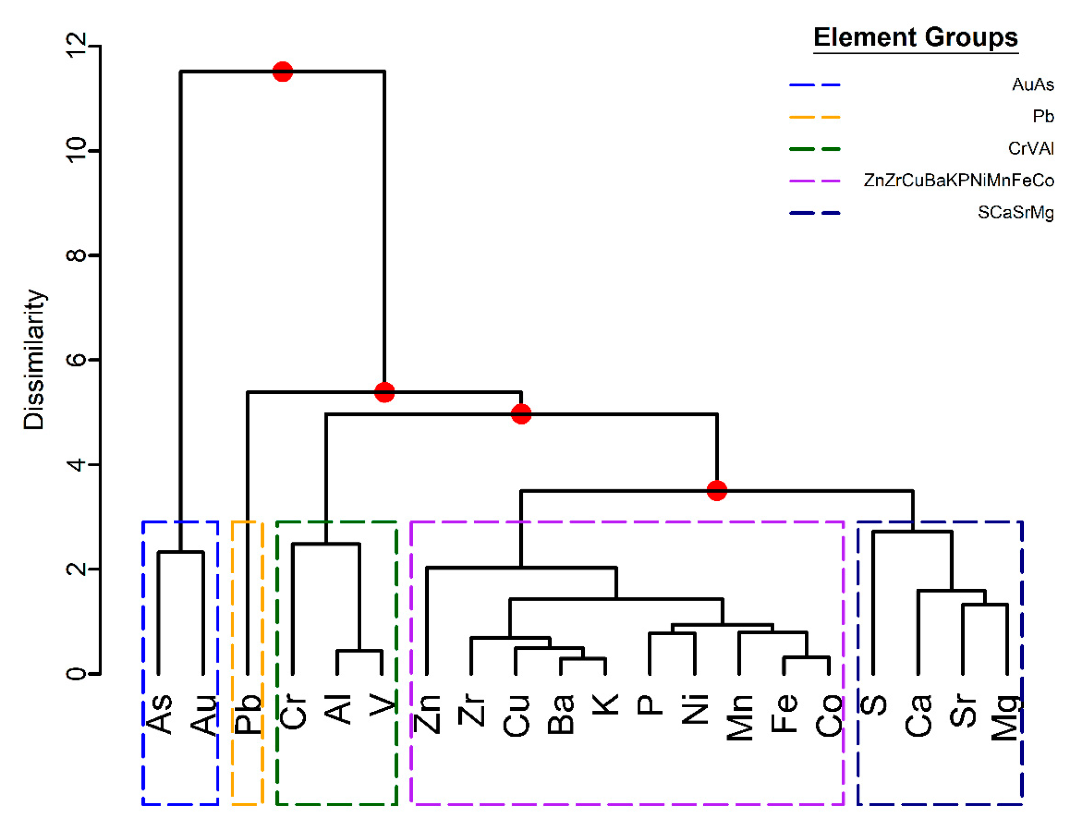
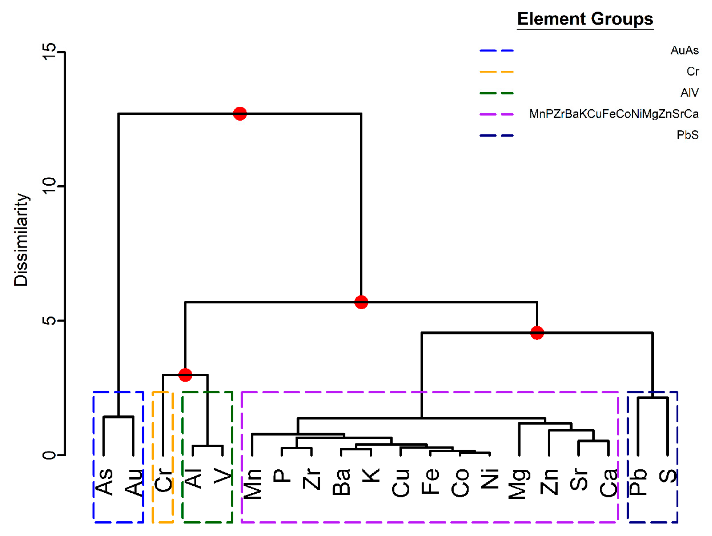
The hierarchical cluster analysis of the geochemical variables shows clusters of elements that can be linked to the Paracatu geochemical attributes, Figure 7. The greatest dissimilarity occurs between the Au-As cluster and the large cluster of the remaining geochemical elements. The Au-As co-dependency is explained by the association of arsenopyrite and gold mineralization at Paracatu [28]. The dissimilarity of Au-As to the other elements indicates that the most evident geochemical variability at Paracatu is related to gold mineralization. The remaining geochemical elements define four clusters whose ratios are affected by a combination of geochemical processes including mineralization, hydrothermal alteration and weathering. For example, Pb has the least co-dependence to the other elements and it is considered its own cluster. Pb is a low field strength element that can be mobilized during weathering processes. The Cr–V–Al cluster represents a group of immobile elements in the phyllite [26,30]. Similarly, the other two clusters can be explained by mineralization and hydrothermal alteration at Paracatu [26]. Accordingly, the groupings suggested by the cluster dendrogram capture geochemical processes expected for the Paracatu deposit and can be used to reduce the 20-part geochemical data to a 5-part subcomposition of dissimilar variables.

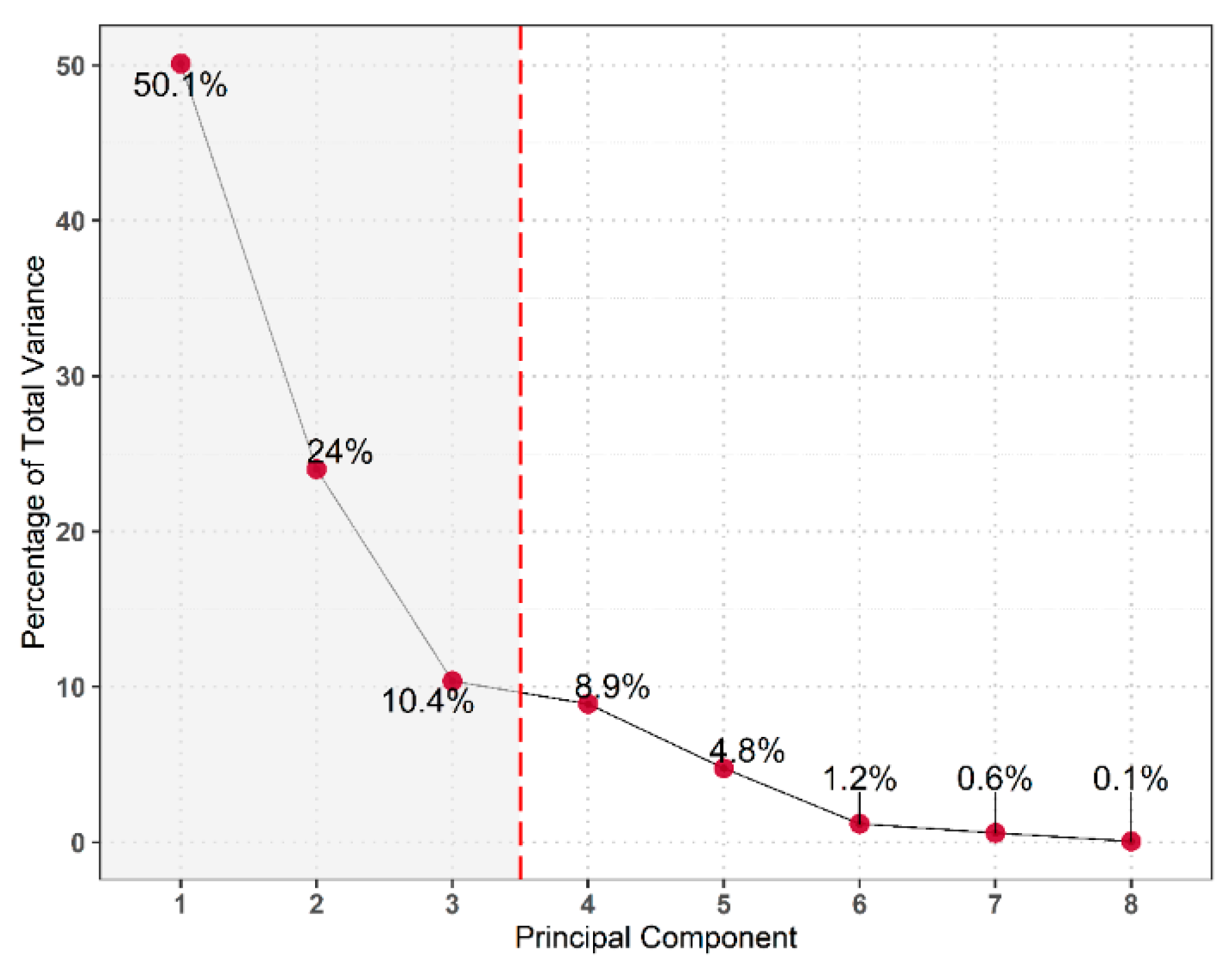
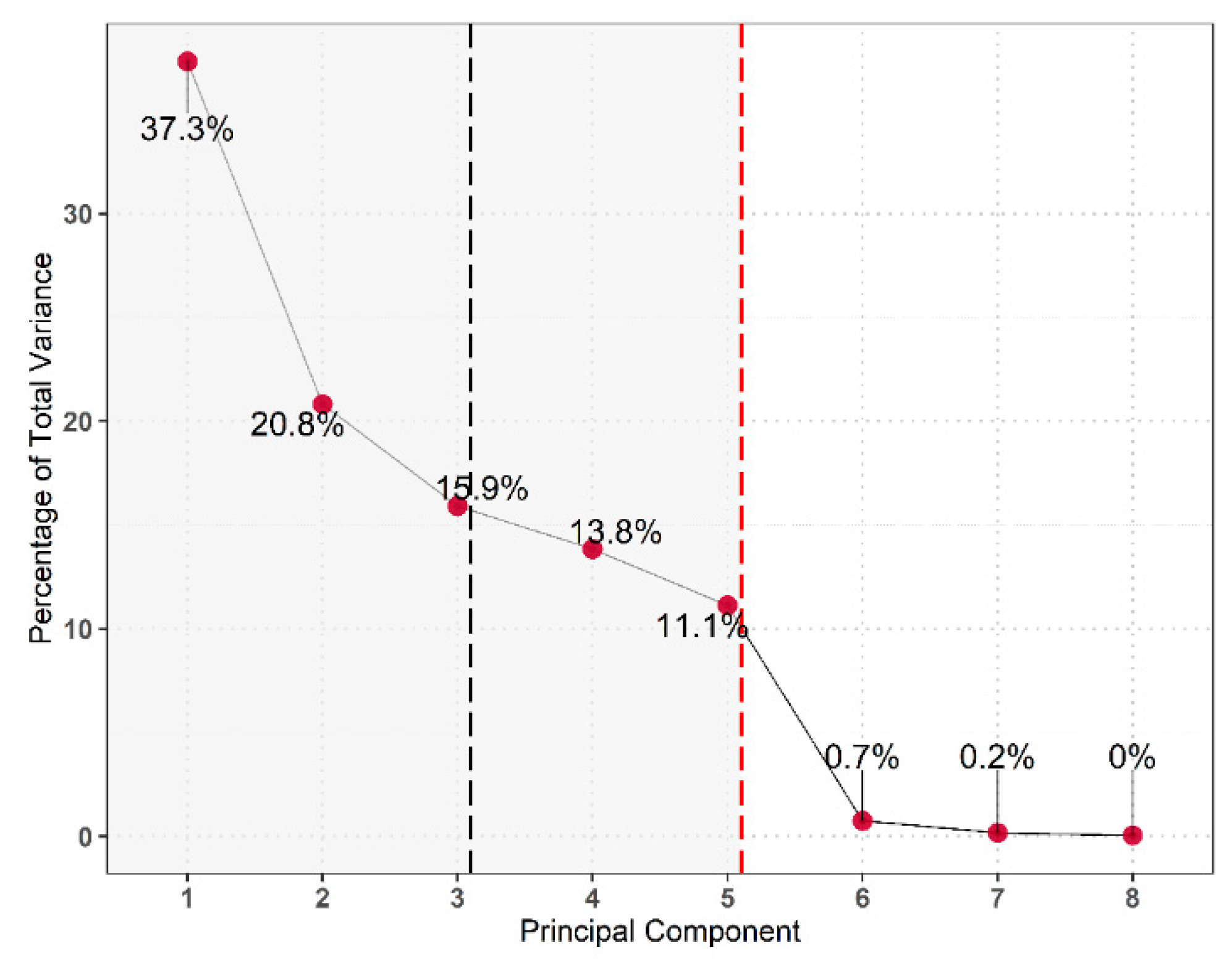
Five composite geochemical variables are created from the hierarchical dendrogram clusters. The joint matrix of compositional data, composite geochemical variables and non-compositional data, BWI, PLSI_AX, RQD and MAGSUSC is used in PCA following the approach of [47] (Section 3.3.1). 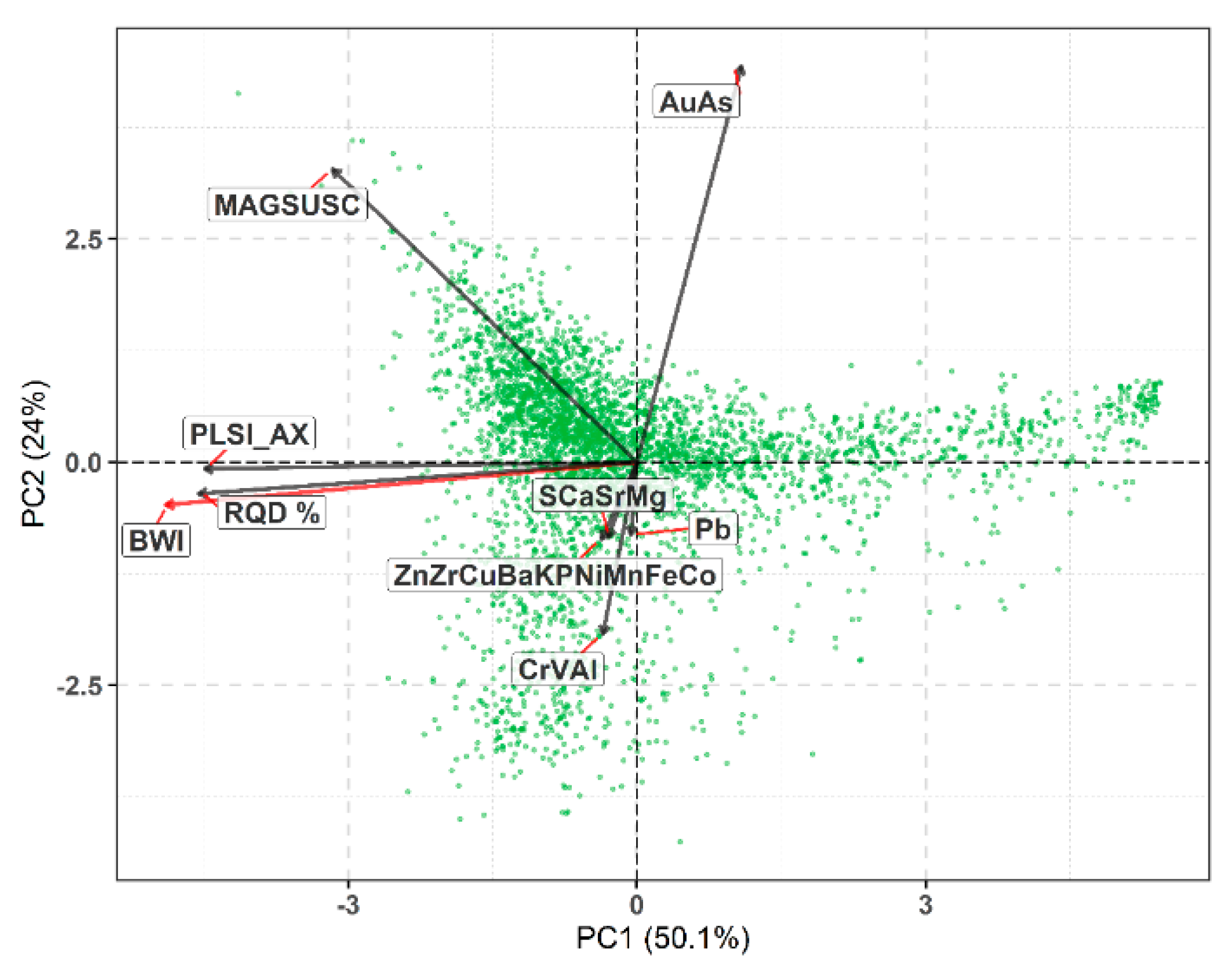The first three principal components capture approximately 85% of the sample variance for weathered and fresh rock observations, Figure 8; the inflection point occurs at PC3. Approximately 50% and 24% of the variance is explained by PC1 and PC2, respectively.

Figure 9 presents the biplot for PC1 and PC2. Both geomechanical variable vectors, PLSI_AX and RQD, have small angles to BWI, which signifies a strong geometallurgical association between rock competency (rock strength and fracturing) and grindability. In contrast, the BWI is less associated with the geochemical variables and MAGSUSC, which is shown by the larger angles between BWI and the respective vectors. MAGSUSC has approximately equal loading from both. The BWI, PLSI_AX and RQD vectors have high loadings on PC1, while the geochemical variables have larger loadings on PC2. Thus, PC1 represents a high degree of variability in the data related to the geomechanical and grindability characteristics at Paracatu. PC1 segregates the data into domains with a large difference in rock competency. The scores representing observations with higher grindability and lower rock strength and competency extend along the positive PC1 axis and fall opposite the direction of BWI, PLSI_AX and RQD vectors. The geometallurgical relationship between BWI and rock competency can be best applied to these observations. PC2 is predominantly a function of geochemical variation represented by relative gold mineralization content at Paracatu. Scores that extend away from AuAs are observations with depleted gold content; observations with a negative PC2 score have a median Au grade of 0.01 ppm compared to a median Au grade of 0.34 ppm for observations with a positive PC2 score. A third grouping of observations occur in the negative PC1-positive PC2 quadrant along the MAGSUSC vector. These scores represent observations with a stronger magnetic signature. Overall, the association of BWI to PLSI and RQD is the relevant geometallurgical relationship found from this PCA.

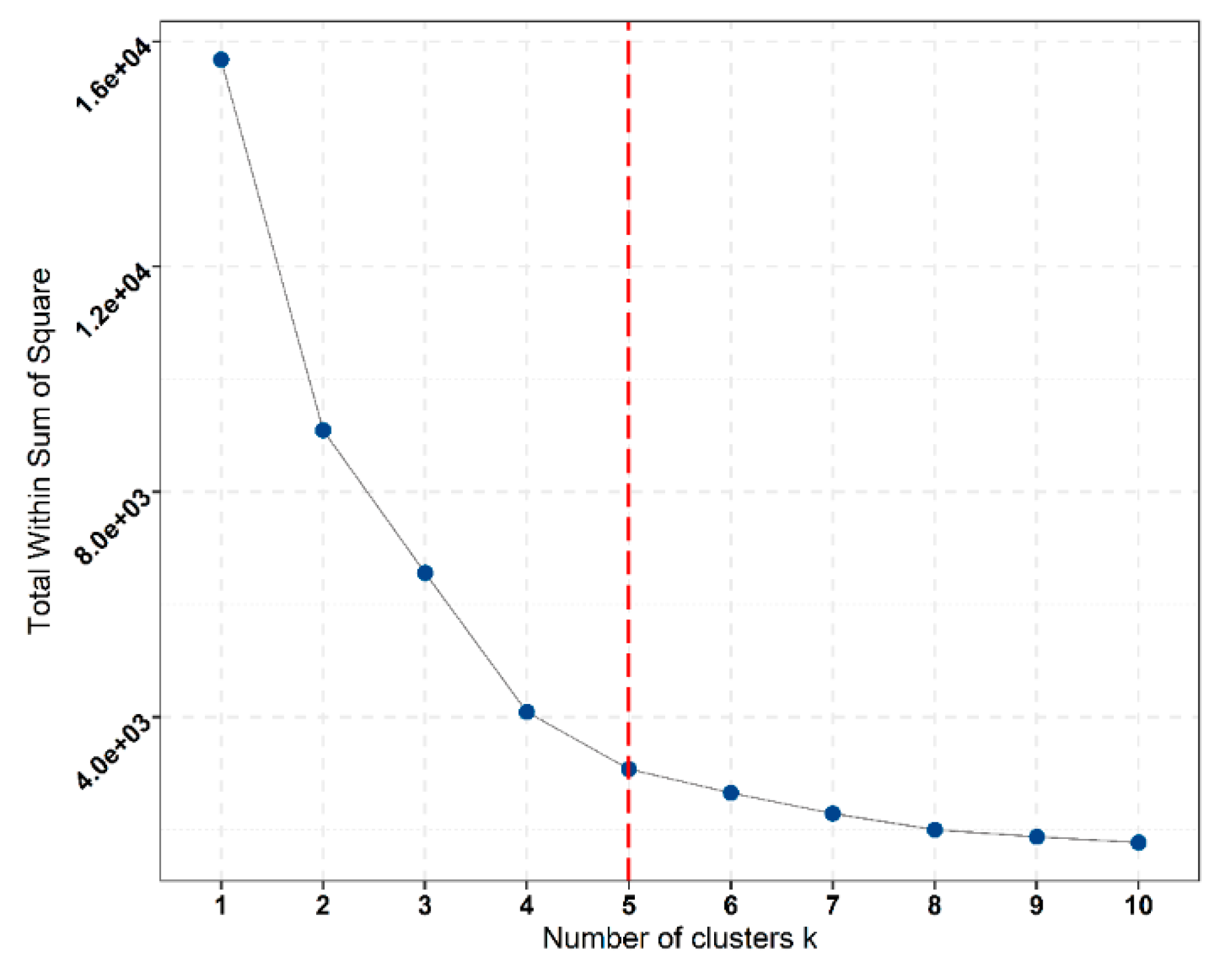
The scores of the first three PCs are clustered using the K-means clustering algorithm to partition the data structure captured by PCA. Changes of the within-cluster sum of squares with the number of K-clusters suggests 4 to 5 significant clusters, Figure 10.

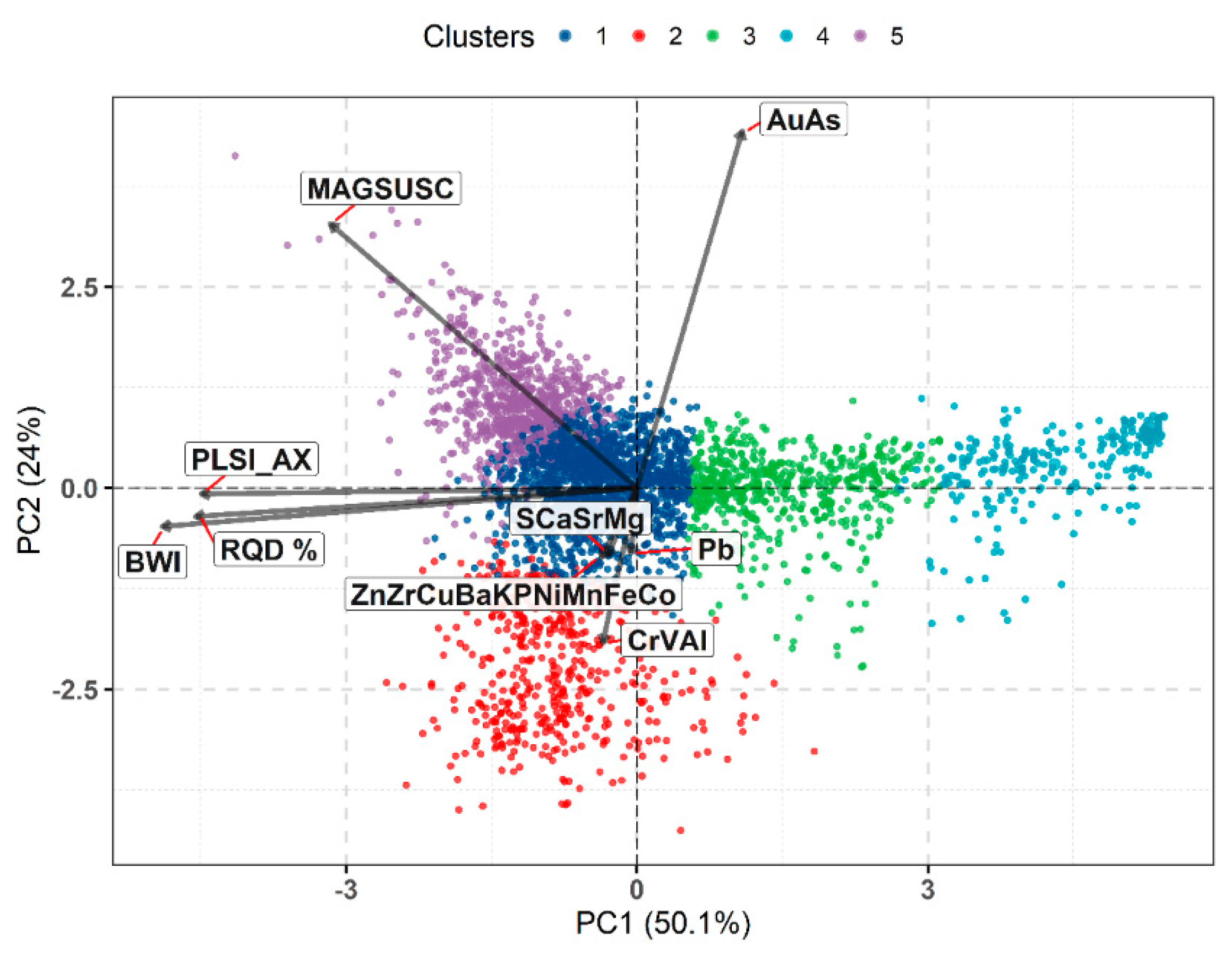
Five clusters are chosen to investigate the possibility of a segmentation in the PC scores that is meaningful for capturing variability in orebody characteristics for geometallurgical domaining. The resulting PCA clusters are well-delineated data driven representations of the score groupings observed on the biplot, cf. Figure 9 and Figure 11.

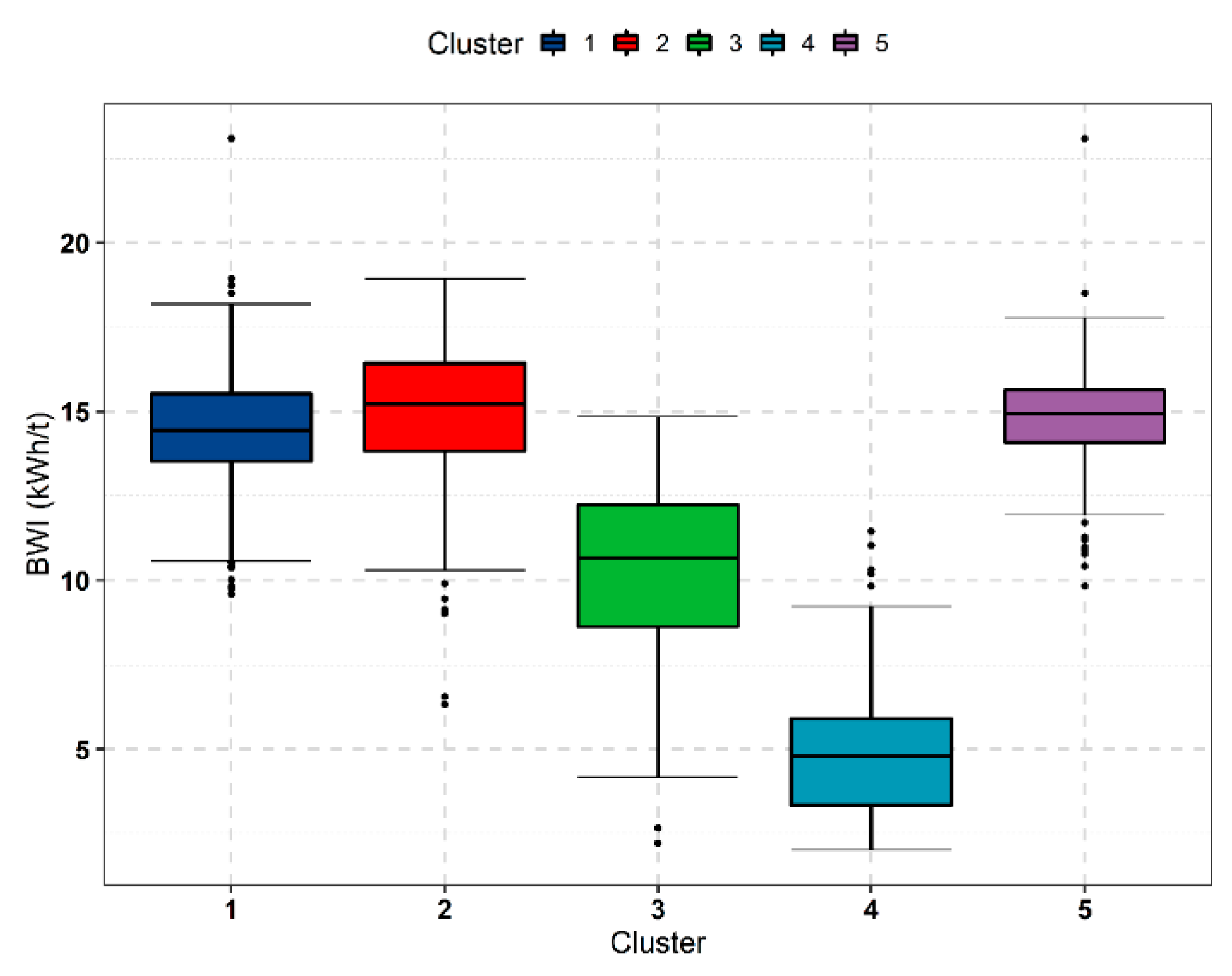
Clusters 3 and 4 represent the observations with the lowest BWI (Figure 12) and therefore lower rock competency and higher grindability. The strong alignment of the two clusters along the PC1 axis indicates that these observations have variability that is best explained by PC1, whose linear combination is dominated by BWI, PLSI_AX and RQD. Therefore, the geometallurgical relationship of BWI to the geomechanical variables is most relevant to clusters 3 and 4. In addition, the median BWI of cluster 4 (c.a. 5 kWh/t) is lower than that of cluster 3 (c.a. 10 kWh/t). The median BWI of the remaining clusters is consistently between 14 and 15 kWh/t. The dispersion of each PCA cluster along the PC1 axis somewhat describes the spread of observations in its corresponding boxplot. For example, cluster 1 and 5 have relatively tight dispersions which are reflected in the boxplots. While clusters 1, 2 and 5 are not distinguished by BWI differences, their dissimilarities arise from other orebody characteristics. Cluster 2 represents observations in phyllite with a low ratio of Au and As to the immobile Cr, V and Al. Cluster 5 observations cluster around the MAGSUSC vector and have a median MAGSUSC value of 1.98 compared to a value 0.72 for the other clusters. It is likely that cluster 5 observations represent the magnetic pyrrhotite of the Paracatu ore. Cluster 1 is generally equidistant along PC2 but has higher PC2 scores than cluster 2. Cluster 1 also extends into the negative PC1 axis, which signifies an increase in rock strength. However, the nounced as those for clusters 3 and 4. This reasoning, combined with the appreciable difference intrend of BWI, PLSI_AX and RQD vectors in comparison to the cluster axes of 1, 2 and 5 is not as pro BWI between the two sets of clusters, signifies a geometallurgical control for observations in clusters 3 and 4 that enables rock strength and fracturing to be related to BWI but which does not affect observations in clusters 1, 2 and 5.

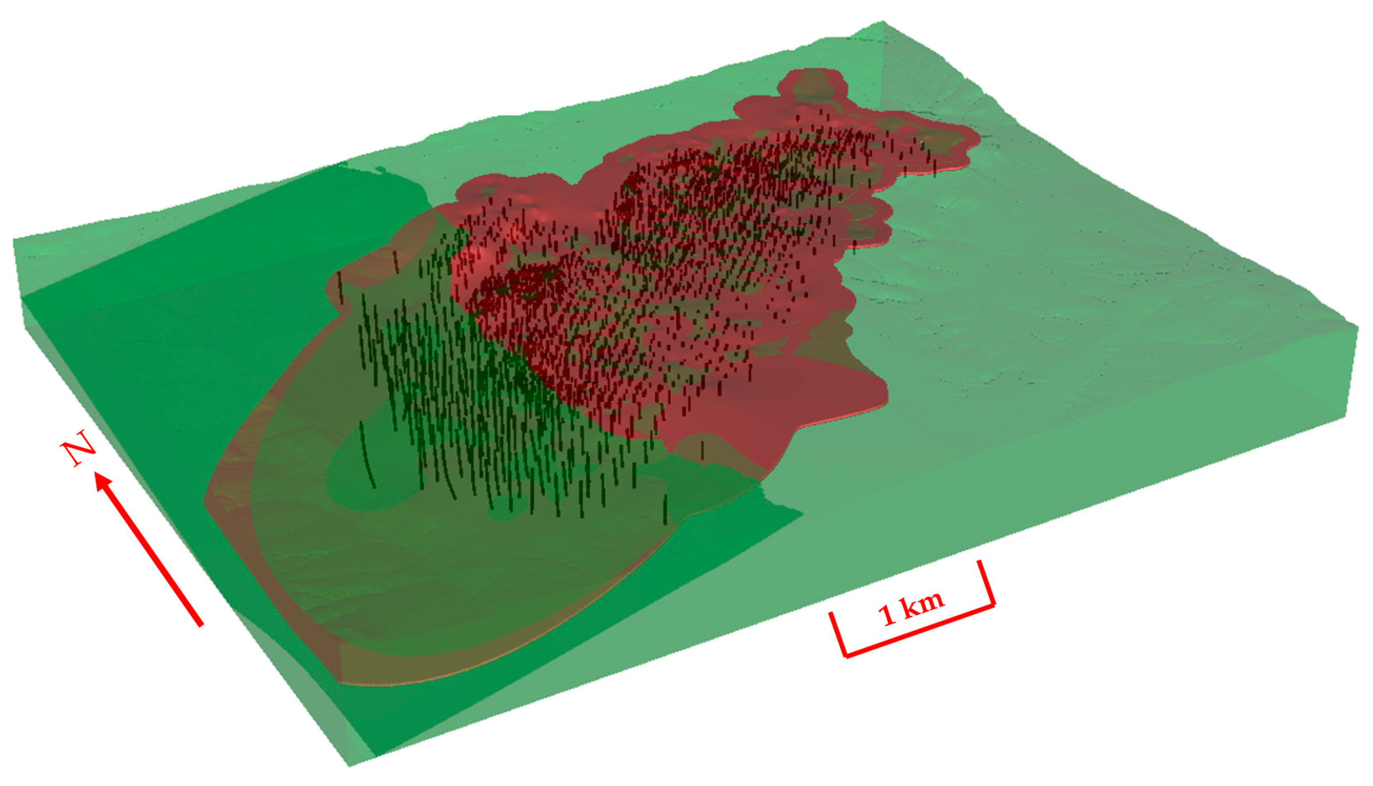
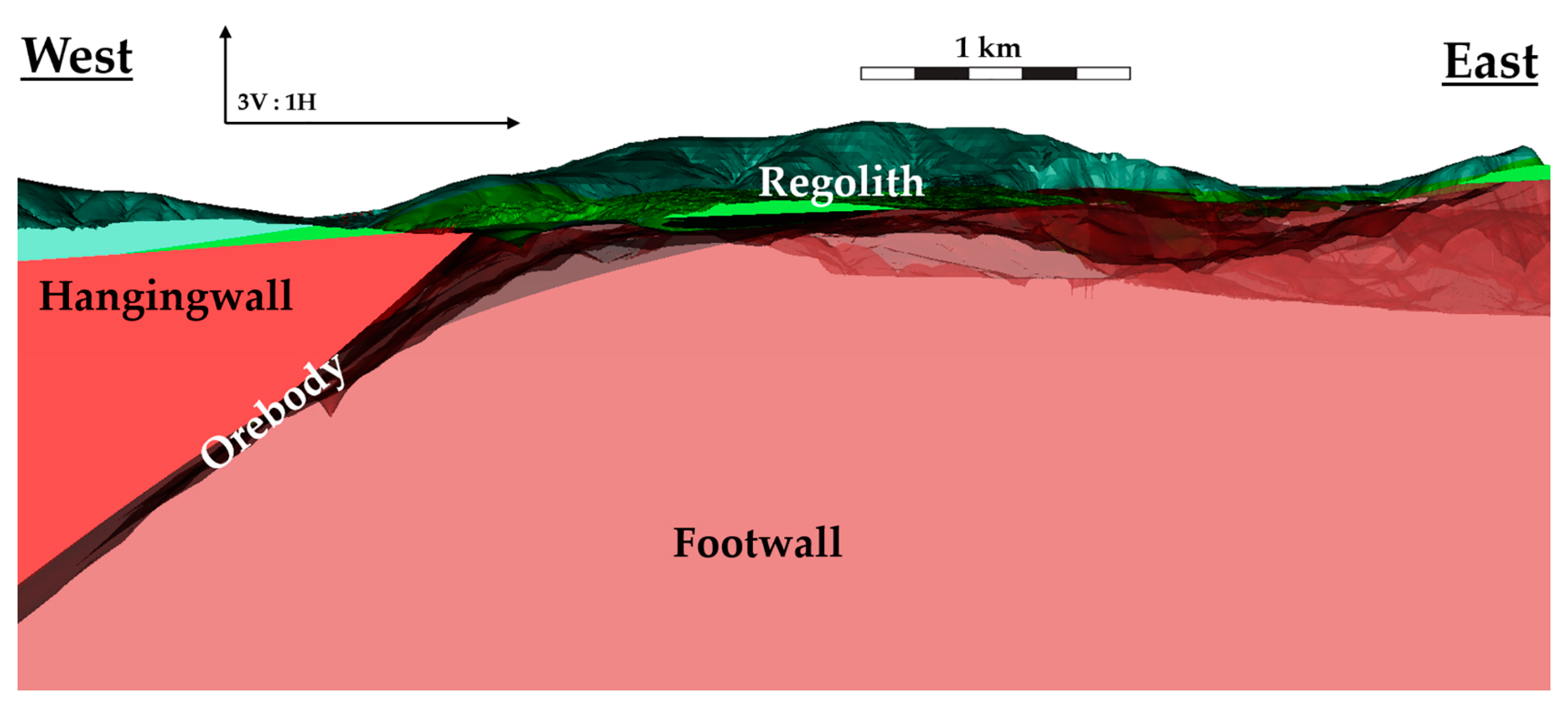
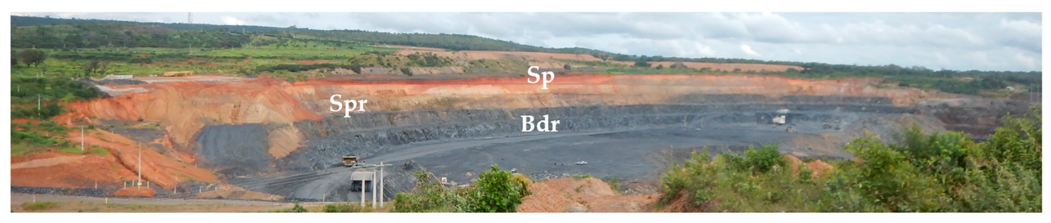
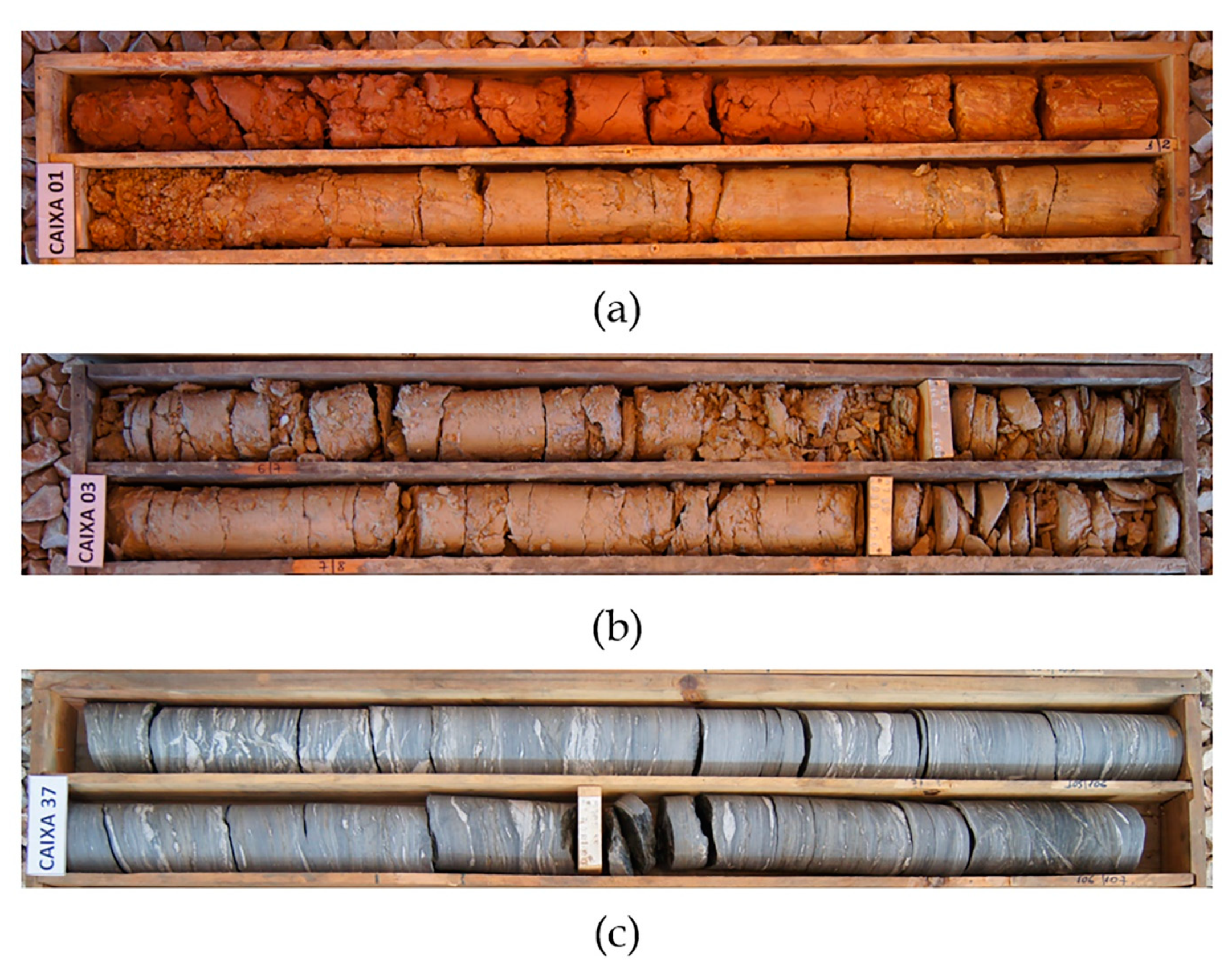
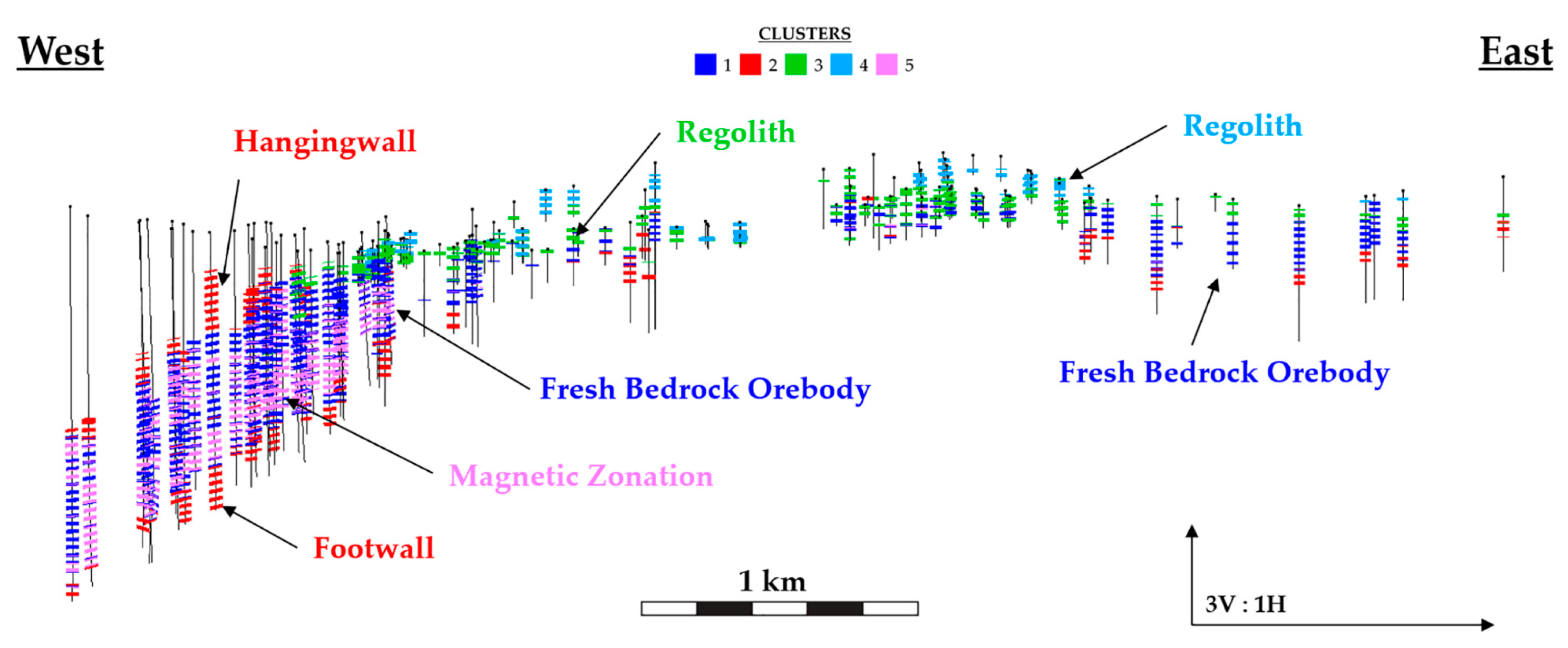
Figure 13 presents a cross-section of the clusters at the Paracatu deposit. The spatial relation of the clusters follows the structure and weathering profile of the Paracatu orebody, c.f. Figure 3. Clusters 3 and 4 represents the upper part of the orebody; which is located in the lateric saprolith, (Figure 5 and Figure 6). Clusters 1, 2 and 5 manifest within the fresh rock of the orebody underlying the saprolith. The significant difference in BWI between the two sets of clusters is caused by extensive lateritic weathering of the deposit (Figure 5). The regolith clusters capture BWI variation between regolith zones of the orebody. Cluster 4 represents the near surface saprolite layer in the regolith given its higher elevation and lower BWI relative to cluster 3. Similarly, the saprock and transition material of lower regolith is defined by cluster 3. The degree of weathering influence on the geomechanical characteristics in the regolith clusters is comparable to its influence on BWI. This results in the large variability captured by PC1 and the considerable contrast in rock competency between the regolith clusters and fresh rock clusters. Thus, the relationship between BWI and PLSI_AX and RQD in the geometallurgical orebody domain identified by the regolith clusters 3 and 4 is attributed to the weathering process. The fresh rock clusters also show distinct spatial patterns that corroborate well with the geological attributes of the orebody. Cluster 2 represents the non-mineralized hanging wall and footwall phyllite characterized by the relatively high content of immobile Cr, V and Al. Clusters 1 and 5 represent the fresh rock observations of the orebody. Cluster 1 has a significant lateral variation in thickness from east to west that follows the dip of the hypogene B2 mineralization domain in the Paracatu orebody. This area of the orebody shows zonations with magnetic cluster 5 mapping the presence of pyrrhotite in the mineralized zone.

Overall, the PCA clusters delineate two orebody domains significant for geometallurgical relationships to BWI: the regolith and the fresh rock. In addition, the PCA clusters are validated by the spatial variability in the orebody physical characteristics.

4.2. Analysis of Fresh Bedrock Observations Subset

The PCA and K-means cluster analysis is effective in capturing variations in the orebody weathering profile related to the upper saprolite, transitional saprock and fresh rock. However, a significant part of the orebody is hosted in the fresh rock, within which weathering is not present as the geometallurgical control. Therefore, to investigate geometallurgical relationships in the fresh rock domain, the analytical workflow is repeated for only the observations in fresh rock clusters. Accordingly, the regolith clusters 3 and 4 are removed from the dataset. This results in the retention of n = 2750 observations for 762 BWI samples located in the fresh rock clusters 1, 2 and 5.

Hierarchical clustering was applied to a variation matrix created for fresh rock observations, Figure 14 and

Table A2. Variation matrix for fresh rock observation data subset. Smallest number column-wise indicates strongest dependence.

Element	Al	As	Au	Ba	Ca	Co	Cr	Cu	Fe	K	Mg	Mn	Ni	P	Pb	S	Sr	V	Zn	Zr
Al		4.04	4.39	0.53	0.57	0.46	0.40	0.47	0.46	0.53	0.39	0.68	0.49	0.52	1.83	1.39	0.71	0.12	0.68	0.54
As	4.04		1.34	2.42	2.84	2.38	5.12	2.54	2.42	2.28	2.89	2.26	2.46	2.69	2.52	1.94	2.65	4.05	2.69	2.52
Au	4.39	1.34		2.69	3.12	2.73	5.45	2.78	2.69	2.58	3.11	2.54	2.72	2.84	3.05	2.22	3.08	4.29	3.09	2.88
Ba	0.53	2.42	2.69		0.38	0.14	1.03	0.16	0.11	0.04	0.20	0.23	0.15	0.24	1.04	0.68	0.43	0.44	0.35	0.24
Ca	0.57	2.84	3.12	0.38		0.32	1.03	0.37	0.27	0.31	0.18	0.37	0.31	0.31	1.39	0.89	0.29	0.51	0.55	0.39
Co	0.46	2.38	2.73	0.14	0.32		0.95	0.12	0.07	0.12	0.14	0.21	0.06	0.20	1.09	0.63	0.42	0.38	0.31	0.20
Cr	0.40	5.12	5.45	1.03	1.03	0.95		1.00	0.97	1.02	0.83	1.32	0.95	1.05	2.45	2.06	1.19	0.32	1.16	1.04
Cu	0.47	2.54	2.78	0.16	0.37	0.12	1.00		0.08	0.16	0.17	0.24	0.11	0.19	1.09	0.60	0.47	0.40	0.35	0.26
Fe	0.46	2.42	2.69	0.11	0.27	0.07	0.97	0.08		0.08	0.08	0.18	0.06	0.15	1.07	0.60	0.40	0.37	0.28	0.19
K	0.53	2.28	2.58	0.04	0.31	0.12	1.02	0.16	0.08		0.17	0.22	0.11	0.22	1.04	0.64	0.39	0.44	0.34	0.19
Mg	0.39	2.89	3.11	0.20	0.18	0.14	0.83	0.17	0.08	0.17		0.25	0.14	0.19	1.30	0.78	0.39	0.30	0.36	0.24
Mn	0.68	2.26	2.54	0.23	0.37	0.21	1.32	0.24	0.18	0.22	0.25		0.23	0.28	1.21	0.68	0.48	0.65	0.47	0.32
Ni	0.49	2.46	2.72	0.15	0.31	0.06	0.95	0.11	0.06	0.11	0.14	0.23		0.19	1.08	0.64	0.42	0.39	0.32	0.21
P	0.52	2.69	2.84	0.24	0.31	0.20	1.05	0.19	0.15	0.22	0.19	0.28	0.19		1.21	0.74	0.46	0.44	0.44	0.36
Pb	1.83	2.52	3.05	1.04	1.39	1.09	2.45	1.09	1.07	1.04	1.30	1.21	1.08	1.21		1.39	1.34	1.71	0.67	1.26
S	1.39	1.94	2.22	0.68	0.89	0.63	2.06	0.60	0.60	0.64	0.78	0.68	0.64	0.74	1.39		0.94	1.30	0.89	0.78
Sr	0.71	2.65	3.08	0.43	0.29	0.42	1.19	0.47	0.40	0.39	0.39	0.48	0.42	0.46	1.34	0.94		0.67	0.62	0.48
V	0.12	4.05	4.29	0.44	0.51	0.38	0.32	0.40	0.37	0.44	0.30	0.65	0.39	0.44	1.71	1.30	0.67		0.59	0.49
Zn	0.68	2.69	3.09	0.35	0.55	0.31	1.16	0.35	0.28	0.34	0.36	0.47	0.32	0.44	0.67	0.89	0.62	0.59		0.47
Zr	0.54	2.52	2.88	0.24	0.39	0.20	1.04	0.26	0.19	0.19	0.24	0.32	0.21	0.36	1.26	0.78	0.48	0.49	0.47

. In the fresh bedrock, most of the element associations are similar to the associations obtained from clustering weathered and fresh rocks, Section 4.1. The Au-As cluster is retained. Some differences, at a 2.5 level of dissimilarity, include the separation of Cr from Al and V to form its own cluster and the production of a single cluster from the combination of Ca, Sr and Mg with the ZnZrCuBaKPNiMnFeCo cluster determined from the clustering of weathered and fresh rocks, as shown in Figure 6. In addition, Pb and S show more similarity in the fresh rocks, relative to the weathered and fresh counterparts. These differences in Pb may well be explained by mobility of Pb and S in the weathering profile, which results in dissimilar relationships when the entire dataset is considered. Five compositional geochemical variables are created based on the cluster dendrogram: AuAs; Cr; AlV; MnPZrBakCuFeCoNiMgZnSrCa; and PbS.

PCA is applied to a joint data matrix of the five compositional geochemical variables and the aforementioned non-compositional variables. The first three and five PCs capture 74% and 99%, respectively, of the total variability, Figure 15. Two plot inflections occur at PC2 and PC5. PC3, PC4 and PC5 have comparable variance. The lack of a drop-off in variance captured between these three means that it is difficult to retain a number of PCs without resorting to higher dimensions (>3). The first three PCs of the fresh rock analysis equate to the same amount of variance explained by the first two PCs from analysis of the entire dataset. Retaining the first two would only capture ~57% of the sample variance.

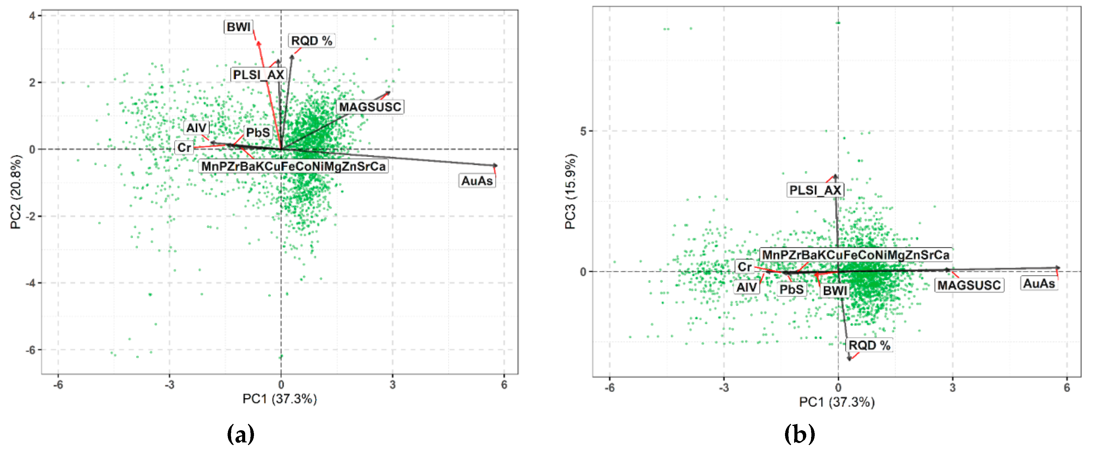
Examining the PC space of the first three components also reveals changes in BWI association, Figure 16. In the PC1-PC2 plane, BWI maintains the relationship with the geomechanical variables found from the PCA of the entire dataset but this association is represented on the lesser PC2 direction, Figure 16a. The BWI-PLSI_AX-RQD relationship is weaker than the first PCA as seen by an increase in the angles between the BWI vector and PLSI_AX and RQD, c.f. Figure 9. The BWI vector shifts slightly towards the geochemical variable vectors. The variance captured by PC2 in this analysis, 20.8%, is much lower than the c.a. 50 % of PC1 which represented the BWI-PLSI_AX-RQD relationship from the first PCA. The PC1 of this analysis shows that the greatest variability in fresh rock, 37.3%, occurs from geochemical and magnetic variations related to gold mineralization. In the PC1-PC3 plane, PC3 is largely controlled by variability in PLSI_AX and RQD (15.9%; Figure 16b); however, this variability does not correlate to variability in BWI or geochemical and magnetic susceptibility.

Overall, the PCA results of the fresh rock observations indicate that variability in this data subset is primarily controlled by geochemical characteristics and is less related to BWI and the other orebody variables. It is likely that PCA, as an unsupervised linear dimensionality reduction technique, may not detect potential associations between BWI and the geochemical characteristics in the fresh rock [3,7] given that BWI associations from PCA at Paracatu are not robust and translate poorly for practical purposes. Therefore, potential non-linear relationships between BWI, geochemical characteristics and the other orebody variables in the fresh rock are investigated using supervised RF classification.

RF variable importance is used to identify orebody variables most significant to BWI for the fresh rock data subset. The PCA cluster membership is added to the dataset as a categorical variable to include geologically validated information about the Paracatu orebody which could improve RF prediction. The ilr variables are defined by using the sequential binary partition of balances between groups of parts established from the fresh rock cluster dendrogram. This results in 19 ilr variables which describe balances between groups of the 20-element subcomposition (Appendix B

Table A3. Isometric log-ratio (ilr) variables or coordinates, defined by balances of the 20-element subcomposition of the fresh rock data subset. Balances are based on sequential binary partitioning of hierarchical clustering results.

Ilr Variable	Binary Partition
ilr1	[ As, Au| Cr, Al, V, Mn, P, Zr, Ba, K, Cu, Fe, Co, Ni, Mg, Zn, Sr, Ca, Pb, S ]
ilr2	[ As| Au ]
ilr3	[ Cr| Al, V, Mn, P, Zr, Ba, K, Cu, Fe, Co, Ni, Mg, Zn, Sr, Ca, Pb, S ]
ilr4	[ Al, V| Mn, P, Zr, Ba, K, Cu, Fe, Co, Ni, Mg, Zn, Sr, Ca, Pb, S ]
ilr5	[ Al| V ]
ilr6	[ Mn, P, Zr, Ba, K, Cu, Fe, Co, Ni, Mg, Zn, Sr, Ca | Pb, S ]
ilr7	[ Mn, P, Zr, Ba, K, Cu, Fe, Co, Ni | Mg, Zn, Sr, Ca ]
ilr8	[ Mn| P, Zr, Ba, K, Cu, Fe, Co, Ni ]
ilr9	[ P, Zr | Ba, K, Cu, Fe, Co, Ni ]
ilr10	[ P| Zr ]
ilr11	[ Ba, K | Cu, Fe, Co, Ni ]
ilr12	[ Ba| K ]
ilr13	[ Cu| Fe, Co, Ni ]
ilr14	[ Fe| Co, Ni ]
ilr15	[ Co| Ni ]
ilr16	[ Mg | Zn, Sr, Ca ]
ilr17	[ Zn| Sr, Ca ]
ilr18	[ Sr| Ca ]
ilr19	[ Pb| S ]

). The ilr variables replace the 5-part composite variables as geochemical variables in the fresh rock data subset.

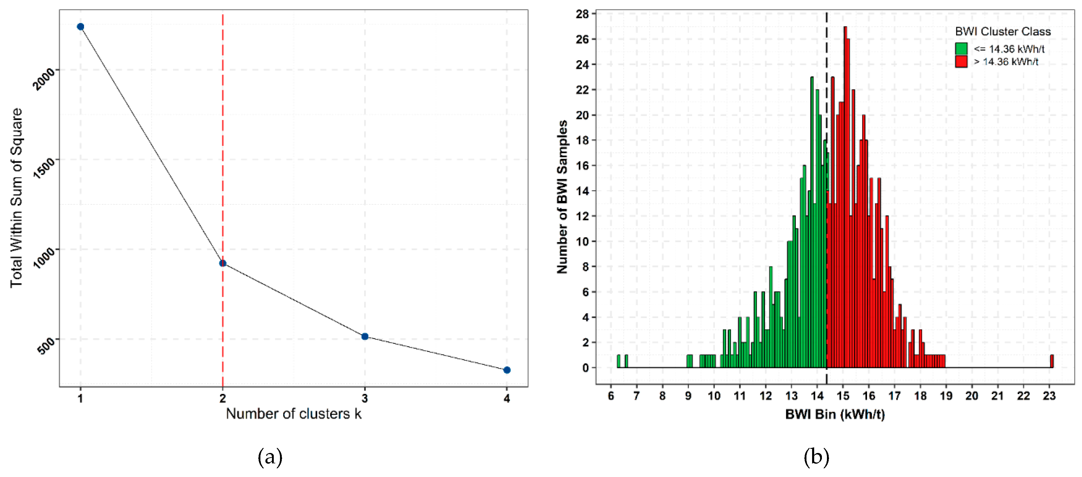
Clustering of BWI sample data from fresh rock indicates that that 2 or 3 classes are suitable for RF classification, Figure 17a. The percentage share of observations in K = 2 clusters is 60–40, which is a better balance than a 52–35–13 percentage share of observations for K = 3 clusters. K = 2 results in two BWI classes, <= 14.36 kWh/t and >14.36 kWh/t, Figure 17b. A BWI operational boundary of 14 kWh/t is suitable for the Paracatu processing circuits (Kinross Gold, personal communication), which is close to the clustered BWI boundary for K = 2. Accordingly, the clustered boundary of 14.36 kWh/t is selected for the reasonable proximity to the operational boundary and improved class balance.

The partitioning of observations into two classes yields n = 1103 observations, corresponding to n = 319 BWI samples, of BWI <= 14.36 kWh/t and n = 1647 observations, corresponding to n = 443 BWI samples, of BWI > 14.36 kWh/t, respectively. The 10-fold CV split of the dataset results in 2484 training observations and 276 test observations for each fold. The first stage of RF hyper-parameter tuning yields a ntree of 800 with the lowest MER over the set of ntree values. In the second tuning stage, an mtry of 14 is selected from a set of mtry values ranging from 3 to 18.

The tuned RF model yields an overall CV classification accuracy of 70%,

Table 3. Confusion matrix, after 10-fold cross-validation (CV), of the random forest (RF) model for BWI classification.

Classification	True Class
Predicted Class	≤14.36 kWh/t	>14.36 kWh/t
≤14.36 kWh/t	572	284
>14.36 kWh/t	531	1363
True Class Total	1103	1647
Predicted Class Total	856	1894
Precision	67%	72%
Sensitivity	52%	83%
Overall Accuracy	70%

. The similar precisions of the two classes, 67% and 72%, suggests that the model is capturing meaningful structure in the orebody variable predictor space for BWI to the same degree for each class, rather than arbitrarily classifying observations. However, the class sensitivities are disproportionate, which suggests an influence of class imbalance. The <= 14.36 kWh/t class, which represents 40% of the dataset, has a much lower sensitivity of 52% than the sensitivity of 83% for the >14.36 kWh/t class. This indicates the RF model is less effective in detecting the minority class.

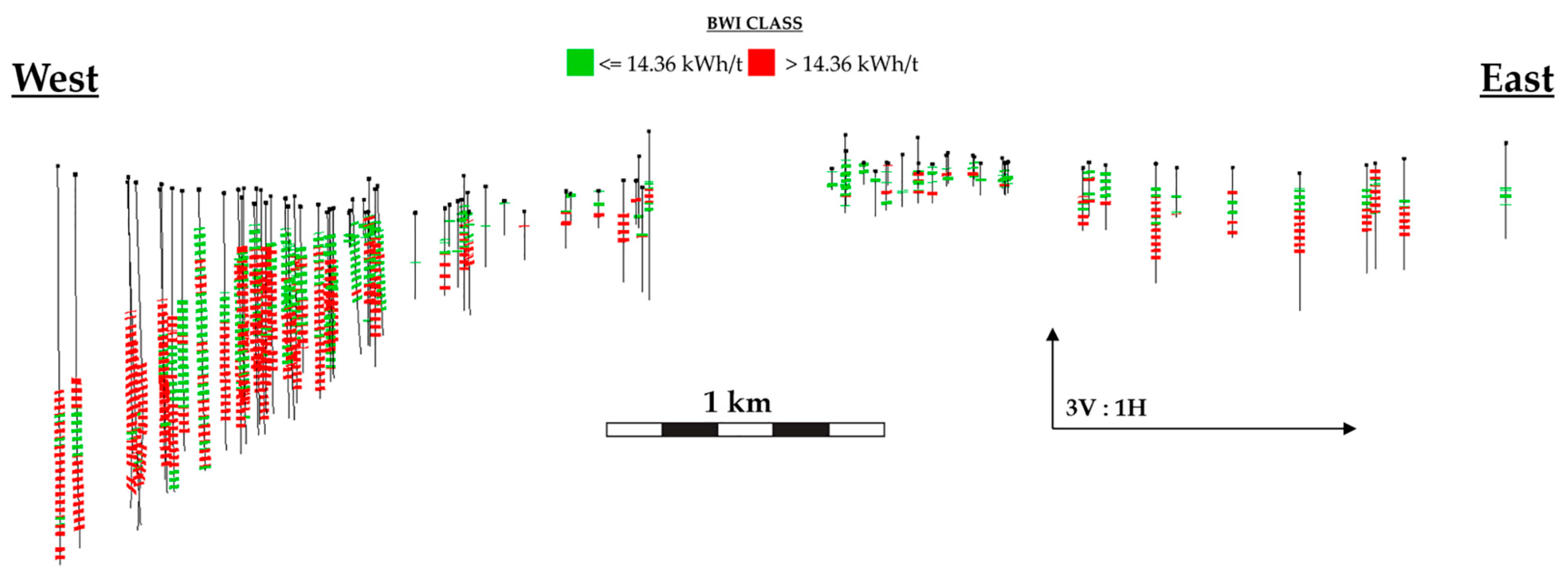
The distribution of each class’ misclassified observations (n = 531 for <=14.36 kWh/t and n = 284 for >14.36 kWh/t) was analyzed to check the BWI margins at which the bulk of misclassifications occur. The 25th, 50th and 75th percentiles are 12.95 kWh/t, 13.71 kWh/t and 14.04 kWh/t, respectively, for the <=14.35 kWh/t misclassified observations. The 25th, 50th and 75th percentiles are 14.75 kWh/t, 15.19 kWh/t and 15.73 kWh/t, respectively, for the > 14.35 kWh/t misclassified observations. Hence, most misclassifications occur for observations near the 14.36 kWh/t boundary, which is inadequate for predictive purposes since this region of BWI requires the greatest level of discrimination for operational decisions. The manifestation of the 14.36 kWh/t class boundary in the orebody, Figure 18, is inconsistent with the geological interpretation of fresh rock clusters 1, 2 and 5 (orebody, hanging wall or footwall and magnetic ore; c.f. Figure 13) and the orebody knowledge detailed in this study (Section 2). The spatial profile of the class boundary shows a general increase in the BWI by depth in the east and an irregular sequence of BWI classes in the west, which is dominated by BWI >14.36 kWh/t. Knowledge of physical variability in the fresh phyllite domain, delineated by PCA clusters 1, 2 and 5.and understanding of BWI test variability at Paracatu should be improved to give a stronger geometallurgical basis for validating BWI classes.

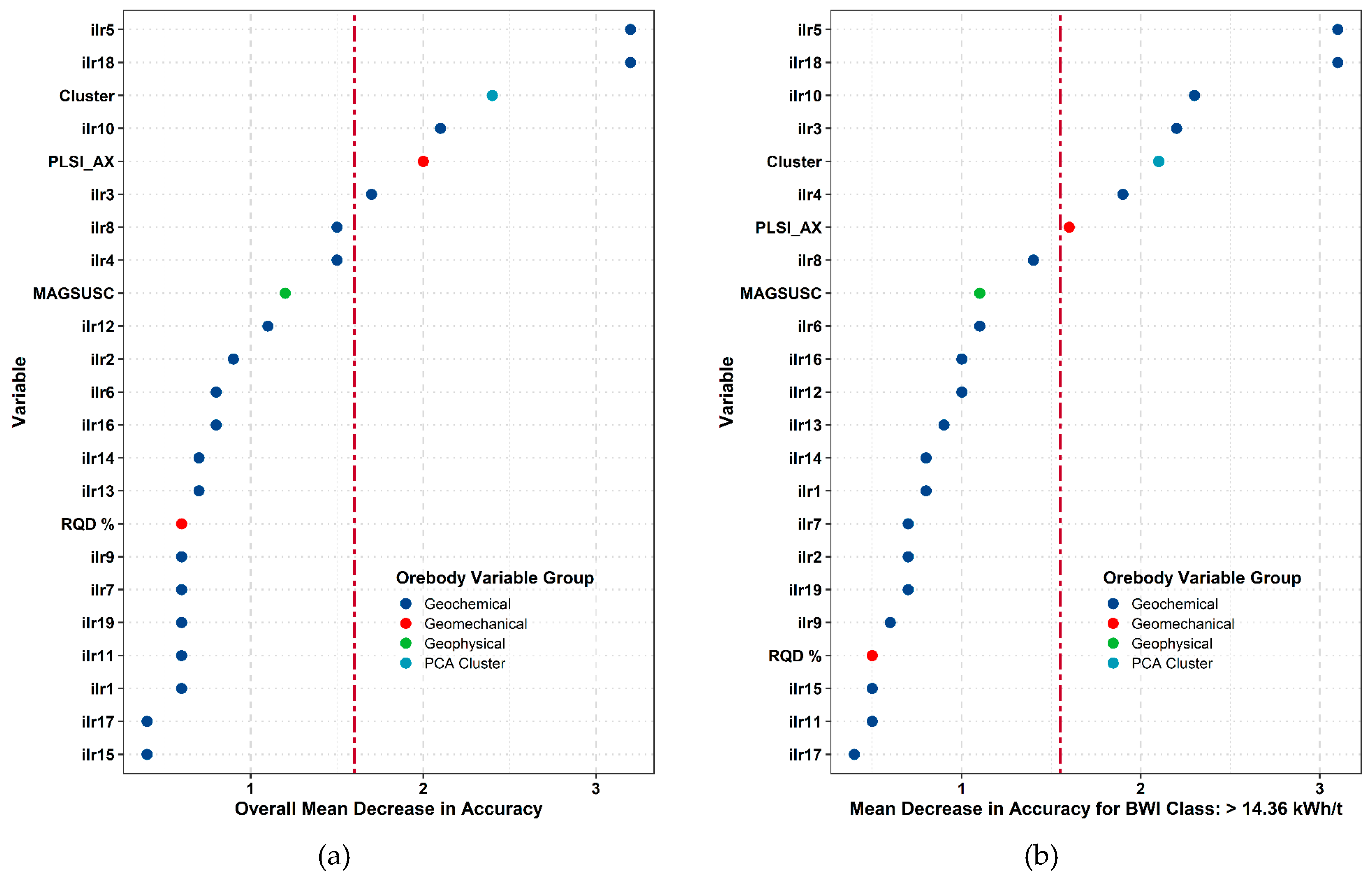
The overall variable importance integrates the importances of both BWI classes, Figure 19. The variable importances of >14.36 kWht is also presented. The <= 14.36 kWh/t class is not considered given its borderline sensitivity of 52%; however, it still has an influence on the overall classification importance as evidenced by slight differences in importance ranking compared to the >14.36 kWh/t class. The PCA cluster and PLSI_AX rank higher in overall classification. In general, RQD is insignificant for BWI classification in fresh rock. Geochemical variables are the most important for classifying fresh phyllite BWI. The ilr 5 and ilr 18 are the two most important geochemical variables. The high importance rankings of ilr 3 and 10 are also consistent between both plots. The ilr 5 (Table A3) is a balance between the immobile Al and immobile V. The ilr 18 is a balance between Sr and Ca. The ilr 10 is a balance between P and the immobile Zr The ilr 3 is a balance involving the immobile Cr and the remaining 19 elements. Accordingly. Therefore, it is likely that subtle variation, all balances important for BWI classification represent associations of immobile and mobile elements s in lithology, mineralization and hydrothermal alteration of the host phyllite exerts control on the BWI classes in the fresh rock.

The variable importances illustrates a shift in BWI association from the geomechanical variables to geochemical variables in the fresh rock domain. The phyllite becomes more intact as it transitions from the regolith into the fresh rock. The fresh phyllite’s grinding resistance is a function of intact strength dictated by mineralogical, textural and microstructural characteristics [32,74,75], which manifest on a centimeter scale down to the micron scale. The ilr variables describe the geochemical variation related to phyllite mineralogy and alteration in the fresh rock. This information can be used to infer small-scale compositional heterogeneity in phyllite matrix characteristics that affect physiomechanical behavior on the micron scale of grinding.

5. Conclusions

The analysis of geometallurgical data is an essential part of the geometallurgical modelling process. Often, the interest is to understand how processing performance indicators relate to variables that measure the orebody’s physiomechanical and geochemical characteristics and how these relationships vary spatially, so that geometallurgical domains can be delineated in the orebody. The quality of this analysis can be compromised if issues related the complex nature of geometallurgical data are not accounted for. The data-driven workflow in this study incorporated data analytics to understand geometallurgical relationships to BWI at Paracatu. This involved the matching of unequal intervals between variables; dimensionality reduction of geochemical multielement data using the variation matrix and hierarchical clustering; representation in unconstrained space of the compositional geochemical groups using ilr balances; and identification of geometallurgical domains and relationships to BWI using data analytics.

Two geometallurgical domains are identified in the Paracatu orebody: the regolith and the fresh rock. In the regolith, the influence of weathering causes a degradation in rock competency that affects, to a similar degree, both phyllite’s resistance to grinding and its’ larger-scale physiomechanical properties. The degradation gives rise to a relationship of BWI to rock strength, PLSI and fracture intensity, RQD. In the fresh rock, compositional variation of the phyllite are linked to variability in the mineralogical, textural and microstructural characteristics of the non-weathered matrix that control small-scale physiomechanical grinding resistance. Geochemical variables, which best capture this compositional variation, are the most important to BWI classification for BWI > 14.36 kWh/t in the fresh rock. In each domain, the relationship between BWI and relevant orebody variables could be further investigated after removing the noisy variables. The validity of the BWI classes should be assessed by improving orebody knowledge in the fresh rock domain, studying BWI test variability and including mineralogical and textural information.

Improvement of the mine geometallurgical model through a data analytics-based approach is beneficial to the mine to mill process optimization. The unsupervised learning can be used to indicate, establish or validate physical characteristics of the orebody that are important for geometallurgical domains depending on the stage of the mine life. The supervised learning can help in identifying complex non-linear geometallurgical relationships. In addition, supervised predictive models for BWI can be trained once adequate knowledge of the geometallurgical characteristics have been defined. At Paracatu, the improved knowledge in the geometallurgical characterization and domains of BWI can be used in mine production planning to feed the milling circuit with a relatively homogeneous ore hardness and reduce fluctuations in circuit throughput and energy consumption.

References

1. Dominy, S.C.; O’Connor, L.; Parbhakar-Fox, A.; Glass, H.J.; Purevgerel, S. Geometallurgy—A Route to More Resilient Mine Operations. Minerals 2018, 8, 560. [Google Scholar] [CrossRef]
2. Hunt, J.A.; Berry, R.F. Economic geology models 3. Geological contributions to geometallurgy: A review. Geosci. Can. 2017, 44, 103–118. [Google Scholar] [CrossRef]
3. Deutsch, C.V. Geostatistical Modelling of Geometallurgical Variables—Problems and Solutions. In Proceedings of the 2nd AusIMM GeoMet Conference, Brisbane, Australia, 30 September–2 October 2013; Dominy, S., Ed.; AusIMM: Melbourne, Australia, 2013; pp. 7–15. [Google Scholar]
4. van den Boogaart, K.G.; Tolosana-Delgado, R. Predictive geometallurgy: An interdisciplinary key challenge for mathematical geosciences. In Handbook of Mathematical Geoscience; Daya Sagar, B., Cheng, Q., Agterberg, F., Eds.; Springer: Berlin, Germany, 2018; pp. 673–686. [Google Scholar] [CrossRef]
5. Keeney, L.; Walters, S.G.; Kojovic, T. Geometallurgical Mapping and Modelling of Comminution Performance at the Cadia East Porphyry Deposit. In Proceedings of the 1st AusIMM GeoMet Conference, Brisbane, Australia, 5–7 September 2011; Dominy, S., Ed.; AusIMM: Melbourne, Australia, 2011; pp. 73–83. [Google Scholar]
6. Newton, M.J.; Graham, J.M. Spatial Modelling and Optimisation of Geometallurgical Indices. In Proceedings of the 1st AusIMM GeoMet Conference, Brisbane, Australia, 5–7 September 2011; Dominy, S., Ed.; AusIMM: Melbourne, Australia, 2011; pp. 247–261. [Google Scholar]
7. Sepúlveda, E.; Dowd, P.; Xu, C.; Addo, E. Multivariate modelling of geometallurgical variables by projection pursuit. Math. Geosci. 2017, 49, 121–143. [Google Scholar] [CrossRef]
8. Deutsch, J.; Palmer, K.; Deutsch, C.V.; Szymanski, J.; Etsell, T.H. Spatial modeling of geometallurgical properties: Techniques and a case study. Nat. Resour. Res. 2016, 25, 161–181. [Google Scholar] [CrossRef]
9. Rossi, M.; Deutsch, C.V. Mineral Resource Estimation; Springer: Berlin, Germany, 2014. [Google Scholar] [CrossRef]
10. Lishchuk, V.; Lund, C.; Lambert, P.; Miroshnikova, E. Simulation of a mining value chain with a synthetic ore body model: Iron ore example. Minerals 2018, 8, 536. [Google Scholar] [CrossRef]
11. Ordóñez-Calderón, J.C.; Gelcich, S.; Oliveira, J.F. Applied Data Analytics on Multi-Element Geochemistry for Pre-Mining Characterization of Geological and Geometallurgical Attributes: Examples from the Rosemont Cu-Mo-Ag Skarn Deposit, Tucson, Arizona. In Proceedings of the 7th CoDaWork Conference, Abbadia San Salvatore Siena, Italy, 5–9 June 2017; Hron, K., Tolosana Delgado, R., Eds.; CoDa Association: Girona, Spain, 2017; pp. 181–194. [Google Scholar]
12. McCoy, J.; Auret, L. Machine learning applications in minerals processing: A review. Min. Eng. 2019, 132, 95–109. [Google Scholar] [CrossRef]
13. Boisvert, J.; Rossi, M.; Ehrig, K.; Deutsch, C.V. Geometallurgical modelling at Olympic Dam mine, South Australia. Math. Geosci. 2013, 45, 901–925. [Google Scholar] [CrossRef]
14. Bhuiyan, M.; Esmaieli, K. Investigating Geometallurgical Relationships by Principal Component Analysis of Compositional and Non-Compositional Data. In Proceedings of the 1st SAIMM Geometallurgy Conference, Cape Town, South Africa, 6–8 August 2018; pp. 193–204. [Google Scholar]
15. Rincon, J.; Gaydardzhiev, S.; Stamenov, L. Coupling comminution indices and mineralogical features as an approach to a geometallurgical characterization of a copper ore. Miner. Eng. 2019, 130, 57–66. [Google Scholar] [CrossRef]
16. Rajabinasab, B.; Asghari, O. Geometallurgical domaining by cluster analysis: Iron ore deposit case study. Nat. Resour. Res. 2018, 1–20. [Google Scholar] [CrossRef]
17. Sepúlveda, E.; Dowd, P.; Xu, C. Fuzzy clustering with spatial correction and its application to geometallurgical domaining. Math. Geosci. 2018, 50, 895–928. [Google Scholar] [CrossRef]
18. Breiman, L. Random forests. Mach. Learn. 2001, 45, 5–32. [Google Scholar] [CrossRef]
19. Strobl, C.; Malley, J.; Tutz, G. An introduction to recursive partitioning: Rationale, application and characteristics of classification and regression trees, bagging and random forests. Psychol. Methods 2009, 14, 323–348. [Google Scholar] [CrossRef]
20. Couët, F.; Goudreau, S.; Makni, S.; Brissette, M.; Longuépée, H.; Gagnon, G.; Rochefort, C. A New Methodology for Geometallurgical Mapping of Ore Hardness. In Proceedings of the 6th SAG Conference, Vancouver, BC, Canada, 20–23 September 2015; Department of Mining and Mineral Process Engineering, University of British Columbia: Vancouver, BC, Canada, 2015. [Google Scholar]
21. Escolme, A.J. Geology, Geochemistry and Geometallurgy of the Productora Cu-Au-Mo deposit, Chile. Ph.D. Thesis, University of Tasmania, Tasmania, Australia, 2016. [Google Scholar]
22. Tiu, G. Classification of Drill Core Textures for Process Simulation in Geometallurgy. Master’s Thesis, Lulea University of Technology, Luleå, Sweden, 2017. [Google Scholar]
23. Kinross Gold Corporation Annual Information Form for the Year Ended December 31, 2018. Available online: https://s2.q4cdn.com/496390694/files/doc_financials/annual/2019/2018-Annual-Information-Form.pdf (accessed on 29 March 2019).
24. Dardenne, M.A. The Brasília Fold Belt. In Proceedings of the 31st International Geological Congress: Tectonic Evolution of South America, Rio de Janeiro, Brazil, 6–17 August 2000; Cordani, U.G., Milani, E.J., Thomaz Filho, A., Campos, D.A., Eds.; FINEP, Fundo Setorial de Petróleo e Gás Natural: Rio de Janeiro, Brazil, 2000; pp. 231–263. [Google Scholar]
25. Pimentel, M.M.; Rodrigues, J.B.; DellaGiustina, M.E.S.; Junges, S.; Matteini, M.; Armstrong, R. The tectonic evolution of the Neoproterozoic Brasília Belt, central Brazil, based on SHRIMP and LA-ICPMS U-Pb sedimentary provenance data: A review. J. S. Am. Earth Sci. 2011, 31, 345–357. [Google Scholar] [CrossRef]
26. Oliver, N.H.S.; Thomson, B.; Freitas-Silva, F.H.; Holcombe, R.J.; Rusk, B.; Almeida, B.S.; Faure, K.; Davidson, G.R.; Esper, E.L.; Guimãraes, P.J.; Dardenne, M.A. Local and regional mass transfer during thrusting, veining and boudinage in the genesis of the giant shale-hosted Paracatu gold deposit, Minas Gerais, Brazil. Econ. Geol. 2015, 110, 1803–1834. [Google Scholar] [CrossRef]
27. Rodrigues, J.B.; Pimentel, M.M.; Dardenne, M.A.; Armstrong, R.A. Age, provenance and tectonic setting of the Canastra and Ibia Groups (Brasília Belt, Brazil): Implications for the age of a Neoproterozoic glacial event in central Brazil. J. S. Am. Earth Sci. 2010, 29, 512–521. [Google Scholar] [CrossRef]
28. Sims, J. Paracatu Project Brazil National Instrument 43-101 Technical Report; Kinross Gold Corporation: Toronto, ON, Canada, 2014. [Google Scholar]
29. Esper, E.; Rugolo, R.; Moller, J.; Akiti, Y.; Pains, A. Morro do Ouro Geological Model with a Metallurgical View. In Proceedings of the 2nd AusIMM GeoMet Conference, Brisbane, Australia, 30 September–2 October 2013; Dominy, S., Ed.; AusIMM: Melbourne, Australia, 2013; pp. 67–74. [Google Scholar]
30. Almeida, B. Geoquímica dos Filitos Carbonosos do Depósito Morro do Ouro, Paracatu, Minas Gerais. Master’s Thesis, Universidade de Brasília, Brasília, Brazil, 2009. [Google Scholar]
31. R Core Team. R: A Language and Environment for Statistical Computing, R Version 3.5.1—“Feather Spray”; R Foundation for Statistical Computing: Vienna, Austria. Available online: https://www.R-project.org (accessed on 12 May 2019).
32. Bhuiyan, M.; Esmaeili, K.; Eden, D. The Influence of Rock Foliation on the Correlation Between the Point Load Strength Index and Comminution Indices at Kinross Tasiast Mine. In Proceedings of the US Rock Mechanics/Geomechanics Symposium, Houston, TX, USA, 26–29 June 2016; ARMA: Alexandria, VA, USA, 2016. [Google Scholar]
33. Tondo, L.A.; Valery, W.; Peroni, R.; La Rosa, D.; Silva, A.; Jankovic, A.; Colacioppo, J. Kinross’ Rio Paracatu Mineracao (RPM) Mining and Milling Optimisation of the Existing and New SAG Mill Circuit. In Proceedings of the 4th SAG Conference, Vancouver, BC, Canada, 23–27 September 2006; Department of Mining and Mineral Process Engineering, University of British Columbia: Vancouver, BC, Canada, 2006; Volume 2, pp. 301–313. [Google Scholar]
34. Semlali, B. Caractérisation et Modélisation Spatiale de la Broyabilité des Massifs Rocheux: Cas de la mine Troilus. Ph.D. Thesis, Universite Laval, Quebec City, QC, Canada, 2007. [Google Scholar]
35. Vatandoost, A. Petrophysical Characterization of Comminution Behavior. Ph.D. Thesis, University of Tasmania, Tasmania, Australia, 2010. [Google Scholar]
36. Ordóñez-Calderón, J.C. Applications of Machine Learning to Model 3D Geological Attributes of Mineral Deposits Using Multi-element Geochemical Data. In Proceedings of the PACRIM 2019 – Mineral Systems of the Pacific Rim Congress, Auckland, New Zealand, 3–5 April 2019; AusIMM: Melbourne, Australia, 2019; pp. 40–42. [Google Scholar]
37. Hunt, J.; Kojovic, T.; Berry, R. Estimating Comminution Indices from Ore Mineralogy, Chemistry and Drill Core Logging. In Proceedings of the 2nd AusIMM GeoMet Conference, Brisbane, Australia, 30 September–2 October 2013; Dominy, S., Ed.; AusIMM: Melbourne, Australia, 2013; pp. 173–176. [Google Scholar]
38. Schouwstra, R.; De Vaux, D.; Muzondo, T.; Prins, C. A Geometallurgical Approach at Anglo American Platinum’s Mogalakwena Operation. In Proceedings of the 2nd AusIMM GeoMet Conference, Brisbane, Australia, 30 September–2 October 2013; Dominy, S., Ed.; AusIMM: Melbourne, Australia, 2013; pp. 85–92. [Google Scholar]
39. Ordóñez-Calderón, J.C.; Gelcich, S.; Fiaz, F. Lithogeochemistry and chemostratigraphy of the Rosemont Cu-Mo-Ag skarn deposit, SE Tucson Arizona: A simplicial geometry approach. J. Geochem. Explor. 2017, 180, 35–51. [Google Scholar] [CrossRef]
40. Palarea-Albaladejo, J.; Martín-Fernández, J.A. Values below detection limit in compositional chemical data. Anal. Chim. Acta 2013, 764, 32–43. [Google Scholar] [CrossRef]
41. Palarea-Albaladejo, J.; Martín-Fernández, J.A.; Buccianti, A. Compositional methods for estimating elemental concentrations below the limit of detection in practice using R. J. Geochem. Explor. 2014, 141, 71–77. [Google Scholar] [CrossRef]
42. Palarea-Albaladejo, J.; Martín-Fernández, J.A. zCompositions—R package for multivariate imputation of left-censored data under a compositional approach. Chemometr. Intell. Lab. 2015, 143, 85–96. [Google Scholar] [CrossRef]
43. Palarea-Albaladejo, J.; Martín-Fernández, J.A. zCompositions: Treatment of Zeros, Left-Censored and Missing Values in Compositional Data Sets. R Package Version 1.1.2. Available online: https://CRAN.R-project.org/package=zCompositions (accessed on 12 May 2019).
44. Aitchison, J. The Statistical Analysis of Compositional Data; Chapman & Hall: London, UK, 1986. [Google Scholar]
45. Egozcue, J.J.; Pawlowsky-Glahn, V. Simplicial geometry for compositional data. In Compositional Data Analysis in the Geosciences: From Theory to Practice; Special Publication 264; Buccianti, A., Matue-Figueras, G., Pawlowsky-Glahn, V., Eds.; Geological Society of London: London, UK, 2006; pp. 145–159. [Google Scholar]
46. Egozcue, J.J.; Pawlowsky-Glahn, V. Groups of parts and their balances in compositional data analysis. Math. Geol. 2005, 37, 795–828. [Google Scholar] [CrossRef]
47. Kynčlová, P.; Filzmoser, P.; Hron, K. Compositional biplots including external non-compositional variables. Statistics 2016, 50, 1132–1148. [Google Scholar] [CrossRef]
48. Grunsky, E. The interpretation of geochemical survey data. Geochem. Explor. Env. A 2010, 10, 27–74. [Google Scholar] [CrossRef]
49. Pawlowsky-Glahn, V.; Egozcue, J.J.; Tolosano-Delgado, R. Modeling and Analysis of Compositional Data; John Wiley & Sons: London, UK, 2015. [Google Scholar]
50. Garrett, R.G. rgr: Applied Geochemistry EDA. R Package Version 1.1.15. Available online: https://CRAN.R-project.org/package=rgr (accessed on 12 May 2019).
51. Galili, T. dendextend: an R package for visualizing, adjusting and comparing trees of hierarchical clustering. Bioinformatics 2015, 31, 3718–3720. [Google Scholar] [CrossRef]
52. Galili, T.; Jefferis, G. dendextend: Extending ‘dendrogram’ Functionality in R. R Package Version 1.9.0. Available online: https://cran.r-project.org/package=dendextend (accessed on 12 May 2019).
53. Ordóñez-Calderón, J.C.; Gelcich, S. Machine learning strategies for classification and prediction of alteration facies: Examples from the Rosemont Cu-Mo-Ag skarn deposit, SE Tucson Arizona. J. Geochem. Explor. 2018, 194, 167–188. [Google Scholar] [CrossRef]
54. van den Boogaart, K.G.; Tolosana-Delgado, R. Analyzing Compositional Data with R; Gentleman, R., Hornik, K., Parmigiani, G.G., Eds.; Springer: Berlin, Germany, 2013. [Google Scholar] [CrossRef]
55. van den Boogaart, K.G.; Tolosana-Delgado, R.; Bren, M. compositions: Compositional Data Analysis. R Package Version 1.40-1. Available online: https://CRAN.R-project.org/package=compositions (accessed on 12 May 2019).
56. Templ, M.; Hron, K.; Filzmoser, P. robCompositions: An R-package for Robust Statistical Analysis of Compositional Data. R Package Version 2.0.6. Available online: https://CRAN.R-project.org/package=robCompositions (accessed on 12 May 2019).
57. Templ, M.; Hron, K.; Filzmoser, P. robCompositions: an R-package for robust statistical analysis of compositional data. In Compositional Data Analysis: Theory and Applications; Buccianti, A., Pawlowsky-Glahn, V., Eds.; John Wiley & Sons: Chichester, UK, 2011; pp. 341–355. [Google Scholar]
58. Hotelling, H. Analysis of a complex of statistical variables into principal components. J. Educ. Psychol. 1933, 24, 417–441. [Google Scholar] [CrossRef]
59. Jolliffe, I.T. Principal Component Analysis, 2nd ed.; Springer: Berlin, Germany, 2011. [Google Scholar] [CrossRef]
60. Johnson, R.A.; Wichern, D.W. Applied Multivariate Statistical Analysis, 6th ed.; Pearson Prentice Hall: Upper Saddle River, NJ, USA, 2007. [Google Scholar]
61. Gower, J.C.; Hand, D.J. Biplots; Chapman and Hall: London, UK, 1996. [Google Scholar]
62. MacQueen, J. Some Methods for Classification and Analysis of Multivariate Observations. In Proceedings of the 5th Berkeley Symposium on Mathematical Statistics and Probability, Berkeley, CA, USA, 21 June–18 July 1967; University of California Press: Berkeley, CA, USA, 1967; pp. 281–297. [Google Scholar]
63. Hartigan, J.A.; Wong, M.A. A K-means clustering algorithm. J. R. Stat. Soc. Ser. C Appl. Stat. 1979, 28, 100–108. [Google Scholar]
64. Hastie, T.; Tibshirani, R.; Friedman, J. The Elements of Statistical Learning: Data Mining, Inference and Prediction, 2nd ed.; Springer: Berlin, Germany, 2009. [Google Scholar] [CrossRef]
65. James, G.; Witten, D.; Hastie, T.; Tibshirani, R. An Introduction to Statistical Learning with Applications in R; Springer: Berlin, Germany, 2013. [Google Scholar] [CrossRef]
66. Kassambara, A.; Mundt, F. factoextra: Extract and Visualize the Results of Multivariate Data Analyses. R Package Version 1.0.5. Available online: https://CRAN.R-project.org/package=factoextra (accessed on 22 August 2017).
67. Wickham, H. ggplot2: Elegant Graphics for Data Analysis, 2nd ed.; Springer: New York, NY, USA, 2016. [Google Scholar]
68. Wickham, H. ggplot2: Create Elegant Data Visualisations Using the Grammar of Graphics. R Package Version 3.1.0. Available online: https://CRAN.R-project.org/package=ggplot2 (accessed on 12 May 2019).
69. Xiao, N. ggsci: Scientific Journal and Sci-Fi Themed Color Palettes for ‘ggplot2’. R package Version 2.9. Available online: https://CRAN.R-project.org/package=ggsci (accessed on 12 May 2019).
70. Breiman, L.; Friedman, J.H.; Olshen, R.A.; Stone, C.J. Classification and Regression Trees; Chapman & Hall: London, UK, 1984. [Google Scholar]
71. Breiman, L.; Cutler, A.; Liaw, A.; Wiener, M. Package ‘randomForest’: Breiman and Cutler’s Random Forests for Classification and Regression. R Package Version 4.6-1.4. Available online: https://cran.r-project.org/web/packages/randomForest/index.html (accessed on 12 May 2019).
72. Kuhn, M. Building predictive models in R using the caret package. J. Stat. Softw. 2008, 28, 1–26. [Google Scholar] [CrossRef]
73. Kuhn, M.; Wing, J.; Weston, S.; Williams, A.; Keefer, C.; Engelhardt, A.; Cooper, T.; Mayer, Z.; Kenkel, B.; Benesty, M.; Lescarbeau, R.; Ziem, A.; Scrucca, L.; Tang, Y.; Candan, C.; Hunt, T.; R Core Team. Package ‘caret’: Classification and Regression Training. R Package Version 6.0-81. Available online: https://CRAN.R-project.org/package=caret (accessed on 12 May 2019).
74. Wills, B.A.; Finch, J. Wills’ Mineral Processing Technology, 8th ed.; Butterworth-Heinemann: Oxford, UK, 2015. [Google Scholar]
75. Mwanga, A.; Rosenkranz, J.; Lamberg, P. Testing of ore comminution behavior in the geometallurgical context—A review. Minerals 2015, 5, 276–297. [Google Scholar] [CrossRef]
Figure 1. Geological setting of the Paracatu deposit. Yellow marker in (a) and (b) locate the mine site. (a) Geological map depicting the Central Domain units and E-verging continental fold-thrust system of the continental Brasilia Fold Belt (modified from [25], after [24]). (b) Area in red inset from (a) showing the regional geology and thrust fault at Paracatu (modified from [27]). (c) Inferred, not to scale, stratigraphic column of the Canastra Group [27].
Minerals 09 00302 g001
Figure 2. Perspective view of the lenticular and tabular Paracatu orebody (red) within the host phyllite (green). Drillhole traces of all drilling conducted at Paracatu shown in black. Majority of drillhole plunges are subvertical to vertical.
Minerals 09 00302 g002
Figure 3. Cross-section of the 3D geological model of the Paracatu lithology looking north with a vertical exaggeration (VEX) of 3:1. Perspective thickness includes north to south extent of mine site. Footwall is shown as transparent to illustrate the orebody and overlying regolith.
Minerals 09 00302 g003
Figure 4. Boudinaged quartz veins subparallel to a composite planar fabric, defining a bedding-parallel foliation in zones with high strain.
Minerals 09 00302 g004
Figure 5. Weathering profile exposed at the southwestern part of the Paracatu mine. The vertical profile shows a red saprolite (sp) transitioning downwards into saprock (spr) and fresh bedrock (bdr). Pit bench height is 12.5 m. The panoramic view looks north-north-east (NNE).
Minerals 09 00302 g005
Figure 6. Drillcore samples from the (a) saprolite, (b) saprock and (c) fresh bedrock.
Minerals 09 00302 g006
Figure 7. Dendrogram after hierarchical clustering the variation matrix of a 20-element geochemical subcomposition analyzed in weathered and fresh rock observations. Red points indicate the cluster splits. Codependence among variables decreases from the bottom to the top of the diagram. The top of the colored boxes corresponds to the dissimilarity at which clusters of elements are taken to create composite variables. The variation matrix is available in Appendix A Table A1.
Minerals 09 00302 g007
Figure 8. Scree plot of principal components and their share of explained sample variance. The shaded region behind the red line represents the total variance, ca. 85%, captured by PC1, PC2 and PC3.
Minerals 09 00302 g008
Figure 9. Principal component 1 (PC1) and PC2 biplot of compositional and non-compositional variables for weathered and fresh rock observations. Green data points represent PC scores and the arrow vectors represent the orebody variables. The BWI loading is shown in red for clarity.
Minerals 09 00302 g009
Figure 10. Plot of K = 1 to 10 clusters and the corresponding total cluster variance. The inflection point can be defined at K = 4 or 5. Red line indicates the chosen K = 5.
Minerals 09 00302 g010
Figure 11. Clusters on the PC1-PC2 biplot after K-means clustering of PC1, PC2 and PC3 scores.
Minerals 09 00302 g011
Figure 12. Bond ball mill work index (BWI) boxplots for each principal component analysis (PCA) cluster.
Minerals 09 00302 g012
Figure 13. Cross-section looking north at Paracatu (VEX: 3 to 1). Observations represented by PCA cluster membership within their drillhole sample. Section thickness includes north to south extent of mine site. The physical meaning of clusters to the orebody are shown by annotations.
Minerals 09 00302 g013
Figure 14. Dendrogram of hierarchical clustering results on the variation matrix of fresh rock observations. Red points indicate the cluster splits. Codependence among variables decreases from the bottom to the top of the diagram. The top of the colored boxes corresponds to the dissimilarity at which clusters of elements are taken to create composite variables. The variation matrix is available Table A2.
Minerals 09 00302 g014
Figure 15. Scree plot of principal components and their share of explained sample variance. The shaded region behind the black and red line represents the total variance of 74% and c.a. 99%, captured by PC1 to PC3 and PC1 to PC5, respectively.
Minerals 09 00302 g015
Figure 16. Biplots for fresh rock observations. Green data points represent PC scores and the arrow vectors represent the orebody variables. The BWI loading is shown in red for clarity. (a) Biplot of PC1 and PC2 (57.3% variance). (b) Biplot of PC1 and PC3 (53.2% variance).
Minerals 09 00302 g016
Figure 17. (a) Total within sum of square for K = 2,3 and 4 clusters of BWI sample data. Red line indicates the plot inflection at K = 2. (b) Histogram of BWI sample data with bins of 0.1 kWh/t. The BWI class boundary occurs at 14.36 kWh/t (dashed line).
Minerals 09 00302 g017
Figure 18. Spatial visualization of the BWI classes, <=14.36 kWh/t and > 14.36 kWh/t, obtained from K-means clustering of BWI sample data. Cross-section looking north at Paracatu (VEX: 3 to 1). Observations represented by BWI class membership within their drillhole sample. Section thickness includes north to south extent of mine site.
Minerals 09 00302 g018
Figure 19. RF variable importance plots for (a) Overall classification and (b) >14.36 kWh/t class. Variables are ranked in descending order of importance. The horizontal axis is in percentage decrease in out-of-bag (OOB) classification accuracy after permutation of variables. Red dashed line indicates 50% of the most important variable’s decrease in accuracy. The type of each orebody variable is color coded.
Minerals 09 00302 g019