A Geostatistical Simulation of a Mineral Deposit using Uncertain Experimental Data

Abstract

In the geostatistical modeling and characterization of natural resources, the traditional approach for determining the spatial distribution of a given deposit using stochastic sequential simulation is to use the existing experimental data (i.e., direct measurements) of the property of interest as if there is no uncertainty involved in the data. However, any measurement is prone to error from different sources, for example from the equipment, the sampling method, or the human factor. It is also common to have distinct measurements for the same property with different levels of resolution and uncertainty. There is a need to assess the uncertainty associated with the experimental data and integrate it during the modeling procedure. This process is not straightforward and is often overlooked. For the reliable modeling and characterization of a given ore deposit, measurement uncertainties should be included as an intrinsic part of the geo-modeling procedure. This work proposes the use of a geostatistical simulation algorithm to integrate uncertain experimental data through the use of stochastic sequential simulations with local probability functions. The methodology is applied to the stochastic modeling of a benchmark mineral deposit, where certain and uncertain experimental data co-exist. The uncertain data is modeled by assigning individual probability distribution functions to each sample location. Different strategies are proposed to build these local probability distributions. Each scenario represents variable degrees of uncertainty. The impacts of the different modeling approaches on the final deposit model are discussed. The resulting models of these proposed scenarios are also compared against those retrieved from previous studies that use conventional geostatistical simulation. The results from the proposed approaches showed that using stochastic sequential simulation with local probability functions to represent local uncertainties decreased the estimation error of the resulting model, producing fewer misclassified ore blocks.

1. Introduction

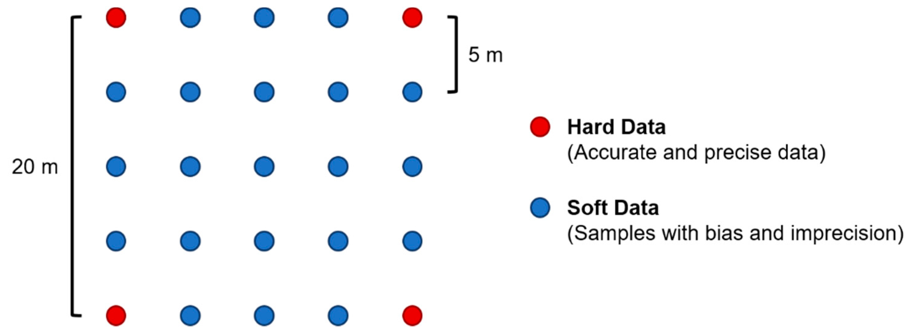
In the mining industry, the economic value of a mineral deposit is estimated using a resource model that is built from the existing direct measurements of the resource of interest. These models are greatly influenced by the quantity, quality, and spatial distribution of the existing direct measurements for the properties of interest (e.g., grades). In general, ore deposit models are built based exclusively on the existing primary data that has been collected from rock core samples and/or logging tools with great precision and accuracy, which are less prone to measurement errors and, therefore, low uncertainty. During the determination of the spatial distribution of this resource, the kinds of data used are generally high quality and provide reliable measurements of the property of interest. Therefore, the data are considered to be reliable hard data with no uncertainty.

Later, during quasi-mining operations, more samples of the property of interest become available. These samples are normally used to fill in the informational gaps that were left over from previous rock core samples, and are often collected along several distinct campaigns from blast holes during the production years, prepared using different protocols, sampled with different equipment, and/or analyzed at different laboratories. Ideally, as the spacing between samples decreases, the uncertainty about the spatial distribution of the mineral deposit is also reduced. However, due to the abovementioned reasons, this information does not have the same quality throughout the entire dataset or within the existing rock core samples. Therefore, it is common to observe different statistical populations formed by readings of the same geological attribute when sampled, prepared, and/or assayed by distinct protocols. These analyses often produce different results when compared with the high quality measurements from the core analysis. From a modeling point of view, lower quality data is frequently considered to be secondary variables (i.e., soft data).

In the mining industry, it is still a common practice to exclude these uncertain measurements from the long-term and auditable resource models due to their imprecision and the bias they may introduce during the geo-modeling workflow and the final ore deposit model. Whether the soft measurement data should be included or not during the modeling procedure is still an open and relevant scientific question, e.g., [1,2,3,4,5,6,7].

Emery et al. [1] discussed the impact of the lack of accuracy within the available set of measurements for resource and reserve evaluation. This work showed that the quantity of data prevailed over its quality (i.e., the more experimental samples that were analyzed, the more accurate the resource and/or reserve models were, independent of the data quality). Therefore, the characterization of a given ore deposit would be improved if all the data available, even with different degrees of uncertainty, are considered during resource modeling.

An alternative approach to integrate secondary data was proposed by Babak and Deutsch [2]. Their methodology consisted of merging all secondary data into a single super secondary variable, which is then used in the geo-modeling workflow through collocated co-kriging. Leuangthong and Deutsch [8] transformed multiple variables into univariate and multivariate Gaussian variables with no cross-correlation. The transformed variables were then submitted to independent stochastic Gaussian simulation and back transformed to the original variables.

Ribeiro et al. [3] proposed the use of mixed support data (i.e., samples obtained using diamond drill holes, and samples collected using a reverse circulation drilling method) in an iron ore deposit evaluation. Although the results showed a small global bias and high spatial correlation between some variables, in general, the differences in volumetric sample support between the two drilling methods generated a conditional bias and low or no correlation on a local scale. Reuwsaat [4] also discussed the effect of sampling using different supports on the precision and accuracy of iron ore deposit models, demonstrating the importance of the correlation between the variables in the quality of the models.

Minnitt and Deutsch [5] showed the importance of using simultaneously primary, accurate, and precise data together with a more abundant, imprecise, and biased secondary dataset, using cokriging as the estimation technique and a linear model of coregionalization to control the use of the secondary data in the estimation of recoverable reserves of mineral deposit grades. Cornah and Machaka [6], and Donovan [7], using a number of specialized geostatistical tools, most of all cokriging-based techniques, also demonstrated that the use of imprecise or biased (or both) secondary data in mineral resource estimations is recommended if the correlation between the data types can be properly estimated. The geostatistical tools used in these works allowed the use of secondary data without transmitting bias and error through to the final models [7], but the uncertainty associated with the measurements was not properly assessed.

A usual way to integrate secondary information during the geo-modeling workflow of natural resources relies on stochastic sequential co-simulation algorithms [9,10,11,12]. Alternative procedures [13] consider the integration of secondary information in the form of geophysical data through Sequential Gaussian Co-simulation (Co-SGS), but do not consider the physical (or geological) processes between variables (i.e., the secondary data is integrated exclusively considering the statistical criteria). Alternative approaches for joint simulation define a hierarchy of variables, in a process known by Collocated Co-simulation [14].

In this paper, we propose an alternative way to integrate uncertain soft data into the natural resource modeling procedure through stochastic sequential simulation with local probability distribution functions [15]. This approach uses the soft data as a probabilistic model by transforming the existing soft data into local probability distribution functions that represent the existing local uncertainty. These local probability functions may be derived exclusively from the existing secondary data, inferred from analogue geological scenarios, provided by expert knowledge, or a combination of all these options. The distribution types should be directly related to the degree of uncertainty expected for the secondary data in order to reproduce the real conditions of the natural resource and its uncertainty measurements.

In order to evaluate the advantages of integrating uncertainty experimental data in stochastic simulation methods, we compare the results between models resulting from conventional stochastic simulation algorithms (i.e., direct sequential simulation (DSS) and co-simulation (co-DSS)) and from stochastic sequential simulation with local probability distribution, as a way to integrate uncertain experimental data (soft data). We base our comparisons exclusively on the methods related to DSS to ensure that all scenarios are based on the same type of assumptions.

2. Methodology

This study proposed direct sequential simulation with local probability distributions [15] as a modeling technique to include uncertain experimental data consistently during the geo-modeling workflow.

DSS with local probability distribution functions can be considered to be a natural extension of the DSS with joint probability distributions [16]. This geostatistical simulation algorithm was designed to integrate data measurements that have variable degrees of uncertainty in the stochastic sequential simulation workflow. This uncertainty can result from the lack of accuracy and precision in the measurements at each location, and can be expressed by a local probability distribution function.

As with any stochastic sequential simulation technique, the main idea of this simulation algorithm was to generate spatially-correlated data values in a sequential approach. DSS with local probability distribution functions is based on two main steps. In the first step, locations associated with uncertain samples, $(x_{\beta })$, were visited following a random path, generating $N_d$ values from the collocated local distributions $F(z(x_{\beta }))$. Following the guidelines of direct sequential simulation [12], at each location, $(x_{\beta }),$ the local mean and variance were computed using simple kriging conditioned to the existing hard data values, $z(x_{\alpha })$, and to the previously simulated samples from other locations associated with uncertain distributions, $z^s(x_{\beta })$, around a given neighborhood. From the local distribution $F(z(x_{\beta })),$ centered at the local simple kriging estimate:

$$z^s={\sum }_{\lambda }{\lambda }_{\alpha }(x_0)z(x_{\alpha })+{\sum }_{\beta }{\lambda }_{\beta }(x_0)z^s(x_{\beta }),$$

(1)

where the kriging weights, ${\lambda }_{\alpha }$ and ${\lambda }_{\beta }$, are associated with the hard data and the previously simulated uncertain experimental data, respectively, and the local variance is represented by the simple kriging variance. From this auxiliary distribution, a value, $z^s(x_0),$ is drawn at the location of the uncertain experimental data [15].

In the second step, after all uncertain locations were visited and a set of $N_d$ values was generated from the local distributions, the stochastic sequential procedure visits the remaining locations of the model using the conventional direct sequential simulation methodology. The resulting models reproduced the spatial covariances, and the global and local distributions [15], as inferred from the existing certain and uncertain data.

The main question about the usability of this stochastic sequential simulation technique relied on how the local probability distribution functions, $F(z(x_{\beta }))$, were built to properly describe the uncertainty of the existing measurements. These distribution functions can be derived from expert guesses or from auxiliary variables, at another $N_d$ experimental sample locations associated with uncertain measurements of the same property in the framework of the stochastic sequential simulation [15].

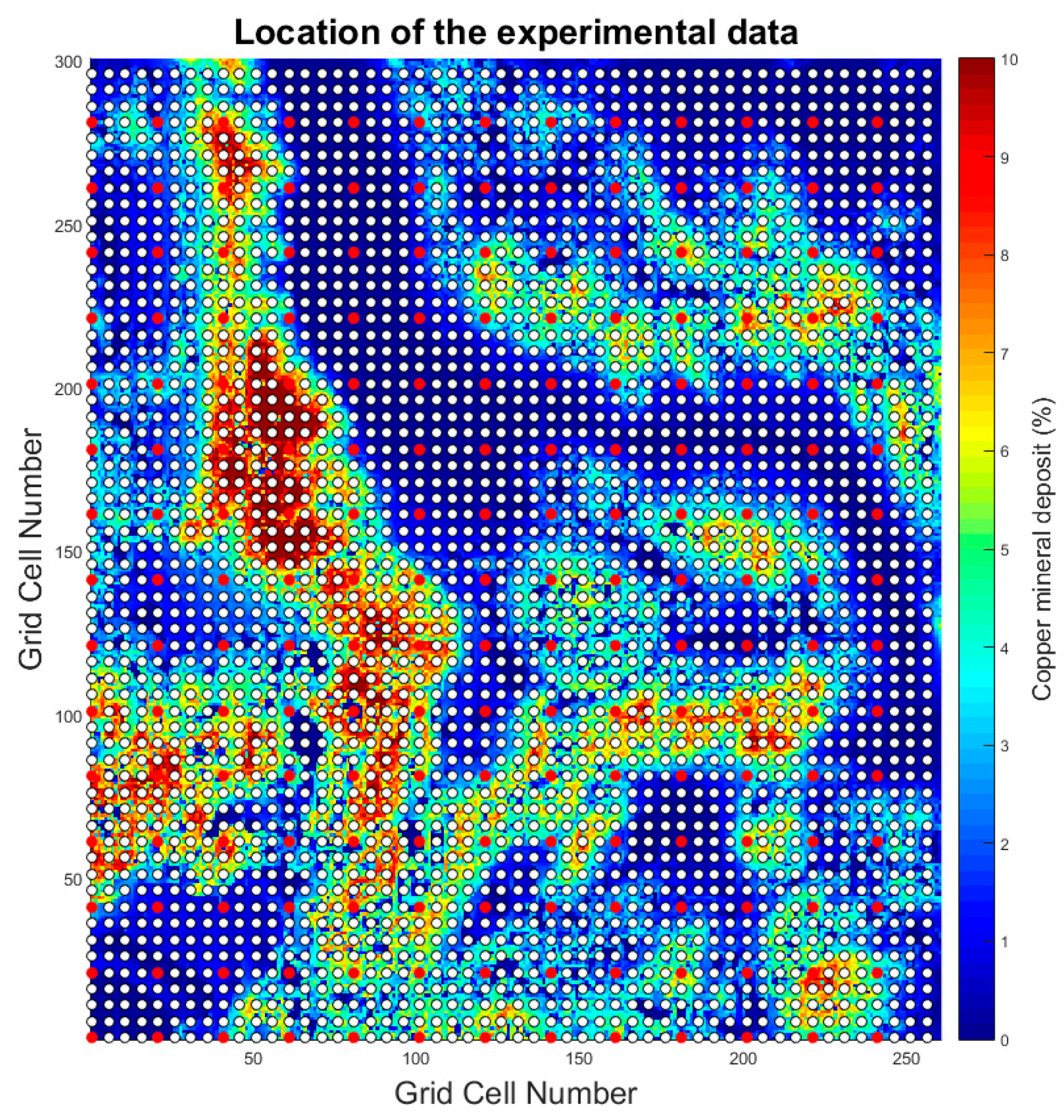
In this study, we proposed alternative strategies to build local probability distributions. The impacts of the different strategies in the resulting models were then compared against each other and contrasted against models resulting from a conventional stochastic sequential simulation algorithm. These different scenarios were applied to a mineral deposit from where a reference model was built from the existing data [17]. This dataset is described in the section below.

In order to assess the impact of the local probability distribution functions, two different approaches were created:

• Experimental local probability distribution functions: the local probability distribution functions were built from 15 soft data samples that were the nearest to the location of the uncertain measurement; and
• Parametric local probability distribution functions: the local probability distribution functions were built using Gaussian distributions with the means and standard deviations inferred from the 15 samples closest to the uncertain location.

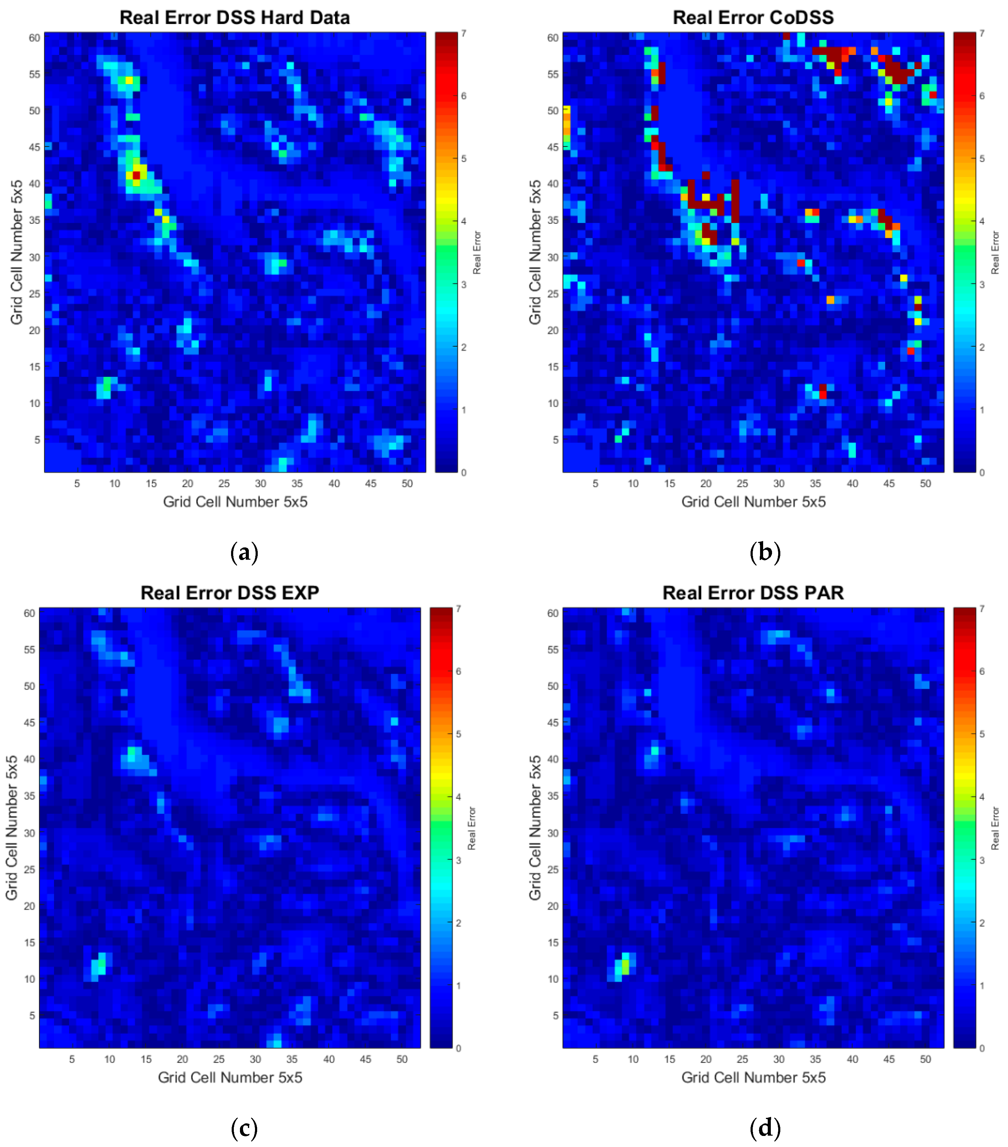
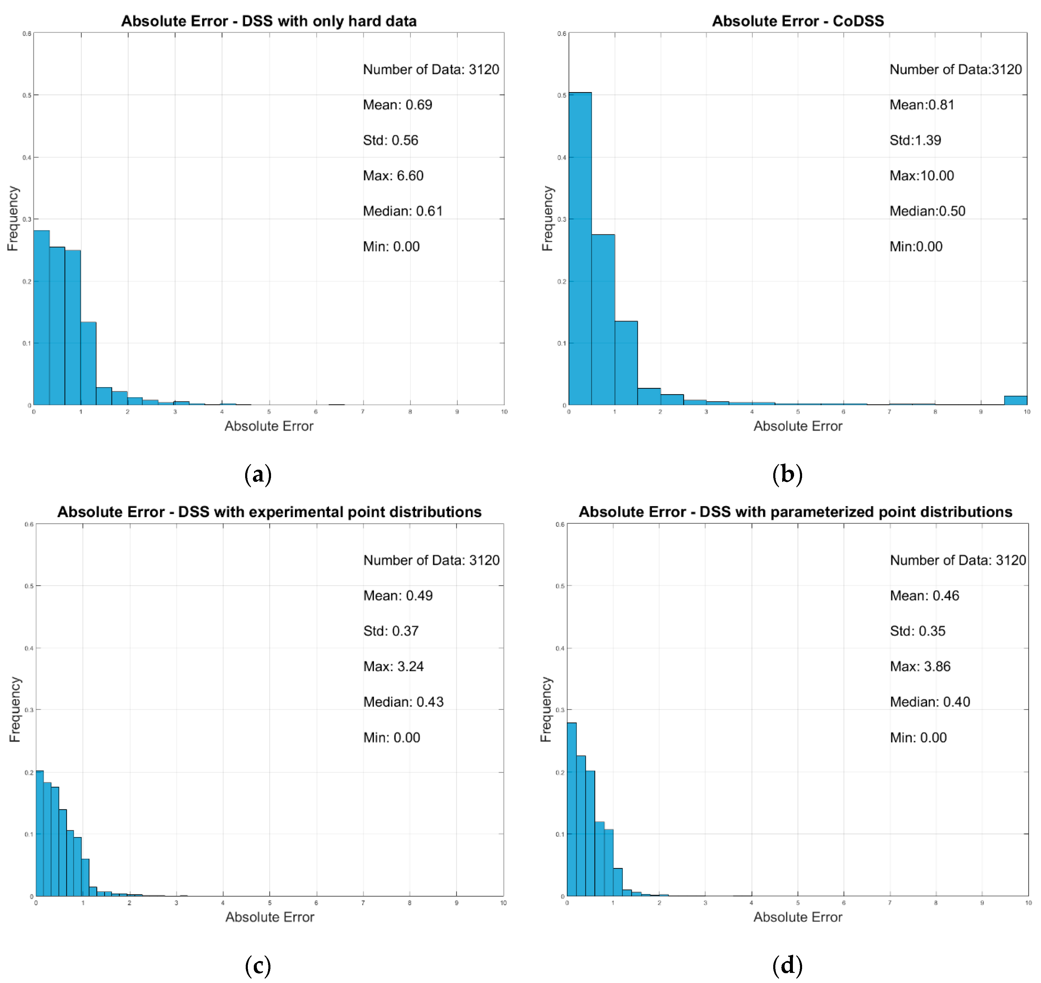
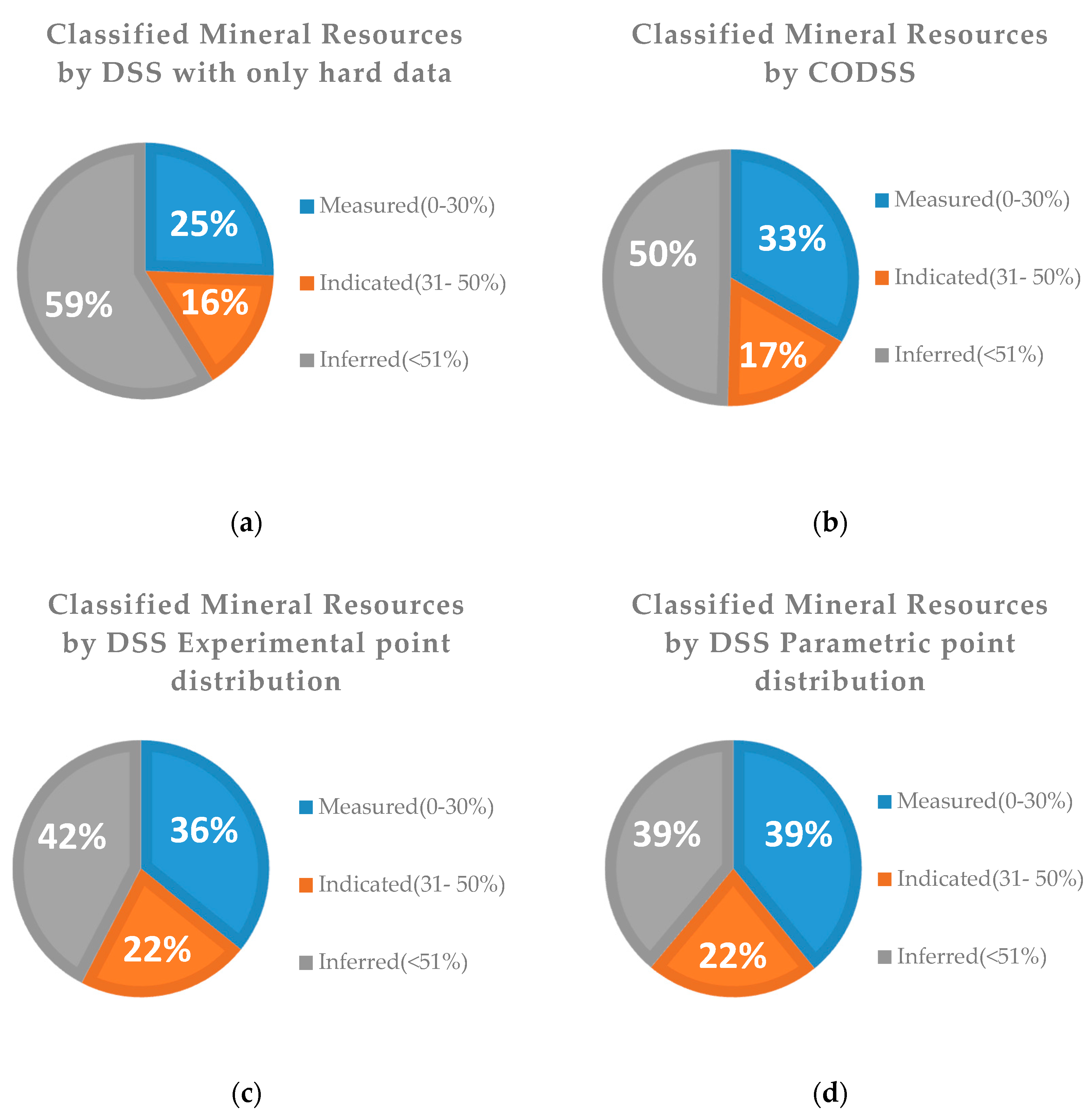
The results of each simulation strategy were compared quantitatively by calculating the error by re-blocking each realization along the reference model, and by computing the proportions of the classified mineral resources as a function of the calculated error.

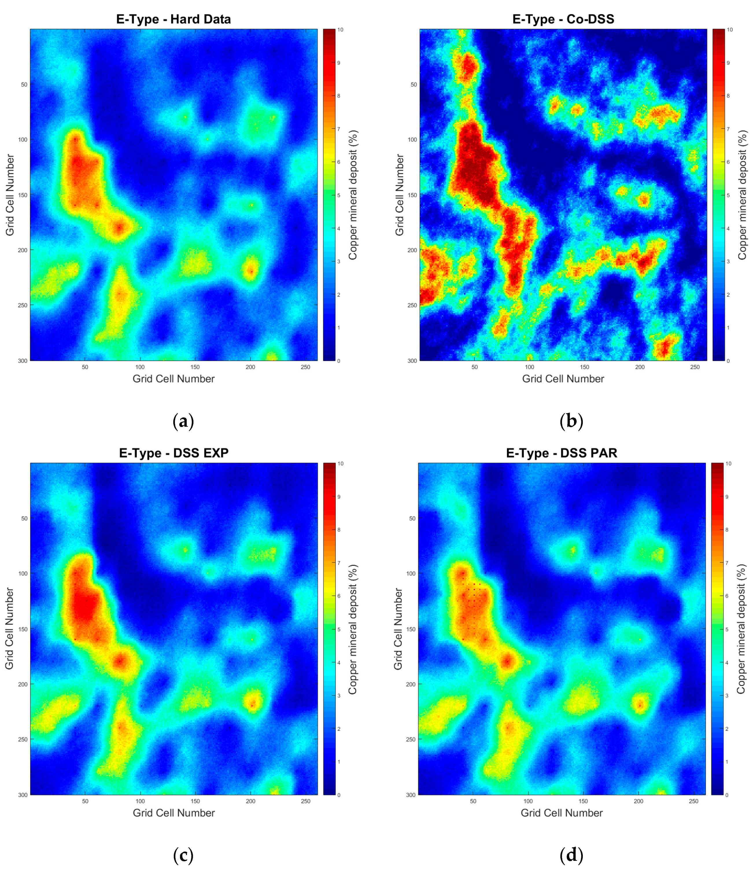
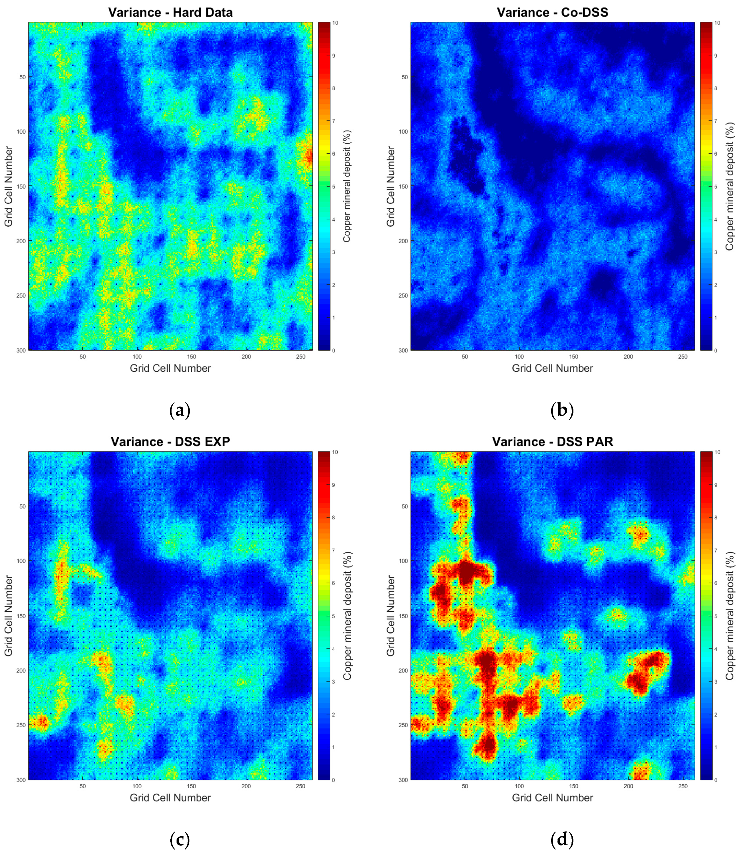
To properly assess the usefulness of the local probability distribution functions and the approaches proposed for a mineral deposit simulation strategy, we compared the following four simulation strategies, using an E-type model (i.e., the mean model of all simulations), the variance model, and the absolute relative errors for each simulation:

• Direct sequential simulation only using the hard data to simulate the mineral deposit;
• Direct sequential collocated co-simulation using the accurate and precise experimental data as the hard data and the uncertain experimental data as the secondary data to simulate the mineral deposit;
• Direct sequential simulation with local probability distribution functions using the accurate and precise experimental data as the hard data and the uncertain experimental data to build experimental local probability distribution functions; and
• Direct sequential simulation with local probability distribution functions using the accurate and precise experimental data as the hard data and the uncertain experimental data to build parametric local probability distribution functions.

3. Application

3.1. Dataset Description

The application example shown here to illustrate the proposed strategy uses the Walker Lake dataset [17], an exhaustive dataset of 78,000 point support samples with a regular sampling grid of 1 m × 1 m (designated from now on as V_Ref_points) and two numerical variables. The original variable, V, from this dataset was scaled up into blocks sized 5 m × 5 m (Figure 1) to represent the block grade distribution of a real copper mineral deposit (designated in this text as V_Ref_blocks). The upscaling resulted in a grid of 3120 blocks, which were considered in this work to be the true block grades.

Within the scope of this case study, the existing dataset was modified in order to retrieve two distinct types of data (Figure 2). The original dataset was sampled into accurate and precise experimental samples, and, therefore, with no uncertainty. These data were regularly spaced at 20 m × 20 m (designated as V_20 × 20), simulating diamond-drill hole samples. The secondary samples, considered to be soft data simulating blast hole samples, were located in a 5 m × 5 m regular grid pattern based on sampling the original dataset. Imprecision and bias were then added to these data (adding variance and error bias) in order to mimic real blast hole samples contaminated with measurement errors [18]. To the original sample data, we either added or subtracted a random relative sampling error of 10% and added a 25% bias (increasing the mean of the grades by 25%).

Table 1. Main statistics of the original reference dataset and the uncertainty dataset used in this work.

Data	No. of Samples	Mean	Standard Deviation	CV	Minimum	Maximum
V_Ref_points	78,000	2.78	2.50	0.90	0.00	16.31
V_Ref_blocks	3120	2.78	2.49	0.89	0.00	15.68
V_20 × 20	195	2.73	2.43	0.89	0.00	10.13
V_5 × 5_+25%	2925	3.44	3.12	0.90	0.00	18.30

shows the main statistics of the datasets used in this work, such as the reference point support dataset (V_Ref_points), the reference block grade distribution (V_Ref_blocks), and the sampled dataset used for the experimental data without uncertainty (V_20 × 20). The hard data samples had mean values similar to the true mean of the reference point support dataset, assuming that it was accurate and precise data, with no biases or imprecision. The datasets, where bias and imprecision were added (designated within the scope of this work as V_5 × 5_+25%) in order to simulate situations of poor quality data, had a mean and standard deviation which were 25% greater than the mean and standard deviation of the reference point distribution dataset (V_Ref_points), thus introducing uncertainty into the grade estimation process.

The cross-correlogram of the hard and soft data showed a correlation of 0.62 (Figure 3). In the mining industry, this correlation is considered to be moderate and suggests that the soft data can be incorporated in the model. However, the correlation indicates possible measurement errors that result from the different techniques and campaigns used for sampling, with all sampling preparation errors associated and poor preparation protocols in laboratory.

The spatial continuity pattern of the property of interest was modeled by combining the hard data (V_20 × 20) and the soft data (V_5 × 5_+25%) using a spherical (Sph) variogram model, with the major direction defined as 157.5° and the minor direction defined as 67.5°:

$${\gamma }_v(h)=1.5+3.0\cdot Sph(1)\cdot \left(\frac{N157SE}{35\mathrm{m}},\frac{N67SE}{25\mathrm{m}}\right)+5.1\cdot Sph(2)\cdot \left(\frac{N157SE}{80\mathrm{m}},\frac{N67SE}{44\mathrm{m}}\right)$$

(2)

This variogram model was used in all the stochastic sequential simulation and co-simulation methodologies compared under the scope of this work. For each simulation strategy, we generated ensembles of 100 realizations in order to compute the statistics from them and compare the results obtained.

3.2. Results

For illustration purposes, the E-type model is shown for the ensemble of 100 realizations that was generated for each modeling strategy (Figure 4). Generally, the averaged model for each ensemble was similar for all the modeling strategies. The main features of interest (i.e., high grade values) appeared in the same locations with approximately the same spatial extent. The main differences between the modeling strategies depended on the grade values. The E-type model obtained from the traditional co-DSS showed a bias toward higher grade values due to the bias that existed in the secondary data, including in the geostatistical simulation (Figure 4b). On the other hand, incorporating the uncertain data in the form of local probability distributions, allowed us to avoid a bias towards the higher grade values (Figure 4c,d). In these cases, the resultant model better resembled the one obtained when exclusively using the experimental hard data without uncertainty (Figure 4a).

Contrary to the mean model, the spatial variability of the computed variance for each ensemble depended greatly on the modeling strategy (Figure 5). The method to integrate secondary uncertain data was a critical choice here. As expected, when using only the experimental data without uncertainty (Figure 5a), the variance within the ensemble depended exclusively on the relative location of the hard data. By using a simple co-DSS (Figure 5b), the spatial variance of the model decreased and the model parameter space was not widely explored (i.e., the variability within the ensemble of one hundred realizations was small). However, the use of local probability distribution functions, built from the existing uncertain experimental data (Figure 5c,d), allowed for a variable degree of variance that was spatially dependent. Note that the variance was not homogeneous throughout the entire field, but depended directly on the type and shape of the local probability distributions used to model the uncertainty associated with the secondary data. The spatial distribution of the variance also depended on the spatial homogeneity of the experimental hard data samples used in the simulations. In the examples shown in Figure 5, high values of variance were mainly located at the boundaries between low and high grade values.

In order to quantitatively compare the results of each method, the E-type model obtained from each simulation technique and the reference model were re-blocked into 5 m × 5 m blocks (Table 1). By changing the scale, we were now able to calculate the absolute relative error (ARE; Equation (3)):

$$Erro{r}_{Real}=\left|\frac{E_{type}-V_{Ref\_Blocks}}{E_{type}}\right|,$$

(3)

where $E_{type}$ represents the averaged model for each simulation technique and V_{Ref_Blocks} represents the true block values.

Figure 6 shows the map for the error of each modeling strategy computed using Equation (3). The ARE map, obtained from the DSS using only the samples without uncertainty (Figure 6a), showed a large, spatially-correlated error. This was in line with what was proposed by Emery et al. (2005) [1]: the bigger the dataset, the better, even though uncertainty errors exist in the samples. The co-DSS (Figure 6b), where the uncertain experimental data were considered as a secondary variable, showed that, on average, higher ARE values were located mainly at the boundaries of the main mineral bodies. Note that these modeling absolute relative errors are directly translated as bias during resource calculation. When incorporating the secondary data as local probability distributions, the relative error decreased for the entire region, inferring that the bias and imprecision of the secondary data were controlled by the local probability distributions used in the stochastic sequential simulations (Figure 6c,d). Also of interest, the high ARE values did not appear at the boundaries of the main mineral bodies.

The information from Figure 6 is summarized using the histogram and the main statistics of each map, as shown in Figure 7. To quantify the bias of the models, we selected the median value of each ARE map as it is a central tendency statistic, less sensitive to extreme values. The error median was 0.61 for the direct sequential simulation with experimental data without uncertainty (Figure 7a), 0.50 for the direct sequential collocated co-simulation (Figure 7b), 0.43 for the direct sequential simulation with experimental point distributions (Figure 7c), and 0.40 for the direct sequential simulation with parameterized point distributions (Figure 7d). As expected, the standard deviation and the mean were smaller in the simulations that used the local probability distribution strategy presented in this work than in the other methodologies investigated in this study for comparison. Thus, the smallest bias was obtained for the direct sequential simulation with parameterized local distribution functions associated with the uncertain secondary data.

Quantifying the ARE of each modeling strategy was an important step since conventional approaches to classify natural resources and mineral deposits in the mining industry tend to use subjective criteria in order to define the limits of measured, indicated, and inferred resources [19].

Table 2. Proportions of the accurately classified mineral resources as a function of calculated relative error.

Classification of Resource	Blocks with Accuracy Error less than
Measured	0–30%
Indicated	31–50%
Inferred	>51%

shows the resource classification criteria established using the calculated ARE for this case study. In this way, we intended to quantify the impact of each modeling technique on the evaluation of the existing resource.

Figure 8 shows the proportions of accurately classified mineral resources using the different simulation sequential strategies and the criteria shown in Table 2. The blocks classified by direct sequential simulation using only hard data (Figure 8a) revealed that this was the least accurate method, with 25% of blocks considered to be measured. Using direct sequential co-simulation, the blocks that were accurately measured increased to 33% (Figure 8b). The strategies based on local probability distributions were more accurate. The resources measured using the direct sequential simulation with experimental point distributions (Figure 8c) increased to 36% accuracy, and with the direct sequential simulation with parameterized point distributions (Figure 8d), the blocks measured accurately increased to 39%. This increase occurred because, when the estimates were done with lower errors, the block misclassification was improved.

4. Conclusions and Recommendations

We investigated the impact of integrating uncertain secondary data into the mineral resource modeling procedure using different DSS modeling strategies. In the example used here, the uncertain experimental data was contaminated by both bias and imprecision in order to mimic real mining conditions.

The results showed that, independent of the quality of the data, more data leads to more reliable models. However, traditional geostatistical modeling approaches, where secondary data are integrated through sequential co-simulation, are not able to properly incorporate the uncertainty present in the data within the resulting models, as these are affected by the bias presented in the secondary data. While the influence of the secondary data can be managed, for example by modifying the correlation coefficient between primary and secondary experimental data (i.e., user-defined correlation coefficients), it has an impact on the reserve calculation.

By using stochastic sequential simulation with local probability functions at the locations of the uncertain data, we were able to fully incorporate the uncertainty presented in the secondary data. The ability to integrate this uncertainty depends on the shape and size of the local probability distributions at the location of the secondary data samples. In this study, we considered two alternative options: using the uncertain data directly or building Gaussian distributions using the statistics retrieved from the uncertain data. The option selected should always be based on the type and quality of the existing data.

References

1. Emery, X.; Bertini, J.P.; Ortiz, J.M. Resource and reserve evaluation in the presence of imprecise data. CIM Bull. 2005, 90, 366–377. [Google Scholar]
2. Babak, O.; Deutsch, C.V. Collocated cokriging based on merged secondary attributes. Math. Geosci. 2009, 41, 921–926. [Google Scholar] [CrossRef]
3. Ribeiro, D.; Monteiro, C.; Cunha, E.; Catarino, M.; Augusto, V.; Gomes, M. Correlation study between reverse circulation and diamond drilling in iron ore deposits. In Proceedings of the 5th World Conference on Sampling and Blending, Santiago, Chile, 25–28 October 2011; pp. 277–285. [Google Scholar]
4. Reuwsaat, J. Estudo de Alternativas de Estimativa Para Jazidas de Ferro Utilizando Dados Heterotópicos; Programa de Pós-Graduação em Engenharia de Minas, Metalúrgica e Materiais, Universidade Federal do Rio Grande do Sul: Porto Alegre, Brazil, 2011. (In Portuguese) [Google Scholar]
5. Minnitt, R.C.A.; Deutsch, C.V. Cokriging for optimal mineral resource estimates in mining operations. J. S. Afr. Inst. Min. Metal. 2014, 114, 189–203. [Google Scholar]
6. Cornah, A.; Machaka, E. Integration of imprecise and biased data into mineral resource estimates. J. S. Afr. Inst. Min. Metal. 2015, 115, 523–530. [Google Scholar]
7. Donovan, P.N. Resource Estimation with Multiple Data Types. Master Thesis, University of Alberta, Edmonton, AB, Canada, 2015. [Google Scholar]
8. Leuangthong, O.; Deutsch, C.V. Stepwise conditional transformation for simulation of multiple variables. Math. Geol. 2003, 35, 155–173. [Google Scholar] [CrossRef]
9. Gómez-Hernández, J.J.; Journel, A.G. Joint Sequential Simulation of MultiGaussian Fields. In Quantitative Geology and Geostatistics, Geostatistics Tróia ’92, Tróia, Portugal, 1992; Soares, A., Ed.; Springer: Dordrecht, The Netherlands, 1993; Volume 5, pp. 85–94. [Google Scholar]
10. Journel, A.G. Modeling uncertainty: Some conceptual thoughts. In Quantitative Geology and Geostatistics, Geostatistics for Next Century; Dimitrakopoulos, R., Ed.; Springer: Dordrecht, The Netherlands, 1994; Volume 6. [Google Scholar]
11. Isaaks, E.H. The Application of Monte Carlo Methods to the Analysis of Spatially Correlated Data. Ph.D. Thesis, Stanford University, Stanford, CA, USA, 1990. [Google Scholar]
12. Soares, A. Direct sequential simulation and cosimulation. Math. Geol. 2001, 33, 911–926. [Google Scholar] [CrossRef]
13. Verly, G.W. Sequential Gaussian Cosimulation: A simulation method integrating several types of information. In Quantitative Geology and Geostatistics, Geostatistics Tróia ’92, Tróia, Portugal, 1992; Soares, A., Ed.; Springer: Dordrecht, The Netherlands, 1993; Volume 5, pp. 543–554. [Google Scholar]
14. Almeida, A.S.; Journel, A.G. Joint simulation of multiple variables with a Markov-type coregionalization model. Math. Geol. 1994, 26, 565–588. [Google Scholar] [CrossRef]
15. Soares, A.; Nunes, R.; Azevedo, L. Integration of Uncertain Data in Geostatistical Modeling. Math. Geosci. 2017, 49, 253–273. [Google Scholar] [CrossRef]
16. Horta, A.; Soares, A. Direct sequential co-simulation with joint probability distributions. Math. Geosci. 2010, 42, 269–292. [Google Scholar] [CrossRef]
17. Isaaks, E.H.; Srivastava, R.M. An Introduction to Applied Geostatistics; Oxford University Press: New York, NY, USA, 1989; p. 561. [Google Scholar]
18. Araújo, C.; Costa, J. Integration of different-quality data in short-term mining planning. Rem: Revista Escola de Minas. 2015, 68, 221–227. [Google Scholar] [CrossRef] [Green Version]
19. Araújo, C.; Costa, J.; Koppe, V.; Soares, A. Reducing error in short term grade prediction including imprecise and inaccurate data. In Proceedings of the 24th World Mining Congress, Rio de Janeiro, Brazil, 18–21 October 2016; pp. 80–89. [Google Scholar]
Figure 1. Exhaustive Walker Lake dataset [17] and the experimental data locations used in this work (red filled circles: samples without measurement errors; white filled circles: samples with measurement errors).
Minerals 09 00247 g001
Figure 2. Schematic representation of the modifications performed to the original exhaustive dataset. Two types of data were considered: samples without and with measurement errors.
Minerals 09 00247 g002
Figure 3. Omnidirectional cross-correlogram for hard data and soft data.
Minerals 09 00247 g003
Figure 4. E-type of the 100 simulations generated for each simulation strategy used: (a) direct sequential simulation with only hard data, (b) direct sequential collocated co-simulation, (c) direct sequential simulation with experimental point distributions, and (d) direct sequential simulation with parameterized point distributions.
Minerals 09 00247 g004
Figure 5. Variance of the 100 simulations for each simulation strategy used: (a) direct sequential simulation with only hard data, (b) direct sequential collocated co-simulation, (c) direct sequential simulation with experimental point distributions, and (d) direct sequential simulation with parameterized point distributions.
Minerals 09 00247 g005
Figure 6. Map of the absolute relative errors for each simulation strategy used: (a) direct sequential simulation with only hard data, (b) direct sequential collocated co-simulation, (c) direct sequential simulation with experimental point distributions, and (d) Direct sequential simulation with local distribution functions.
Minerals 09 00247 g006
Figure 7. Histogram of the absolute error for each simulation strategy used: (a) direct sequential simulation with only hard data, (b) direct sequential collocated co-simulation, (c) direct sequential simulation with experimental point distributions, and (d) direct sequential simulation with parameterized point distributions.
Minerals 09 00247 g007
Figure 8. Proportions of the classified mineral resources as a function of the calculated error by using different strategies: (a) direct sequential simulation with only hard data, (b) direct sequential collocated co-simulation, (c) direct sequential simulation with experimental point distributions, and (d) direct sequential simulation with parameterized point distributions.
Minerals 09 00247 g008