Exploratory Analysis of Provenance Data Using R and the Provenance Package


University College London, Gower Street, London WC1E 6BT, UK
Minerals 2019, 9(3), 193; https://doi.org/10.3390/min9030193
Submission received: 17 January 2019
/
Revised: 9 March 2019
/
Accepted: 15 March 2019
/
Published: 22 March 2019
/
Corrected: 8 March 2023
(This article belongs to the Special Issue Heavy Minerals: Methods & Case Histories)
Abstract
:The provenance of siliclastic sediment may be traced using a wide variety of chemical, mineralogical and isotopic proxies. These define three distinct data types: (1) compositional data such as chemical concentrations; (2) point-counting data such as heavy mineral compositions; and (3) distributional data such as zircon U-Pb age spectra. Each of these three data types requires separate statistical treatment. Central to any such treatment is the ability to quantify the ‘dissimilarity’ between two samples. For compositional data, this is best done using a logratio distance. Point-counting data may be compared using the chi-square distance, which deals better with missing components (zero values) than the logratio distance does. Finally, distributional data can be compared using the Kolmogorov–Smirnov and related statistics. For small datasets using a single provenance proxy, data interpretation can sometimes be done by visual inspection of ternary diagrams or age spectra. However, this no longer works for larger and more complex datasets. This paper reviews a number of multivariate ordination techniques to aid the interpretation of such studies. Multidimensional Scaling (MDS) is a generally applicable method that displays the salient dissimilarities and differences between multiple samples as a configuration of points in which similar samples plot close together and dissimilar samples plot far apart. For compositional data, classical MDS analysis of logratio data is shown to be equivalent to Principal Component Analysis (PCA). The resulting MDS configurations can be augmented with compositional information as biplots. For point-counting data, classical MDS analysis of chi-square distances is shown to be equivalent to Correspondence Analysis (CA). This technique also produces biplots. Thus, MDS provides a common platform to visualise and interpret all types of provenance data. Generalising the method to three-way dissimilarity tables provides an opportunity to combine several datasets together and thereby facilitate the interpretation of ‘Big Data’. This paper presents a set of tutorials using the statistical programming language R. It illustrates the theoretical underpinnings of compositional data analysis, PCA, MDS and other concepts using toy examples, before applying these methods to real datasets with the provenance package.
1. Introduction
At its most basic level, sedimentary provenance analysis identifies the mineralogical, chemical or isotopic composition of individual grains, or assemblages of multiple grains in siliclastic sediment. These properties can then be used to group samples of similar affinity, and thereby trace the flow of sediment through a sediment routing system, e.g., [1,2,3,4,5]. Different levels of statistical complexity arise when multiple samples are compared to each other, or when multiple provenance proxies are applied to multiple samples.
Using a number of short tutorials, this paper will introduce several simple but effective exploratory data analysis techniques that can help to make geological sense of ‘Big Data’ in a sedimentary provenance context. The term ‘exploratory’ means that these techniques allow the user to explore the data independent of any prior knowledge about the geological setting [6,7,8,9]. It groups a number of graphical methods to visualise the data and reveal patterns of similarity and differences between samples and variables. This paper will not introduce methods such as discriminant analysis that formally assign samples to pre-defined provenance areas or petrotectonic settings [10,11].
These notes do by no means claim to give a comprehensive overview of exploratory data analysis. The selection of methods presented herein is heavily biased towards techniques that are implemented in a software package for (sedimentary) geology that was created by Vermeesch et al. [12].
provenance is available free of charge at the Comprehensive R Archive Network (CRAN, https://cran.r-project.org/package=provenance), on GitHub (http://github.com/pvermees/provenance), or via http://provenance.london-geochron.com. The package is written in the statistical programming language R, which is available for Windows, Mac OS-X and Linux/Unix. The easiest way to install the latest stable version of the package is to first install R from http://r-project.org and then type the following code at the command prompt (i.e., the ‘>’): ![Minerals 09 00193 i001]()

Once installed, the package can be loaded by typing:![Minerals 09 00193 i002]()

There are two ways to use provenance. The first of these is through a query-based user interface. To access this interface, type:![Minerals 09 00193 i003]()

The main advantage of the query-based user interface is that it does not require any knowledge of R. Its main disadvantage is the relative lack of flexibility and the difficulty to automate complex and/or repetitive tasks. The second way to use provenance is via the R language itself. This is the quicker and more flexible option, whose only downside is a steeper learning curve compared to the query-based interface. This tutorial will help the reader to climb this learning curve whilst explaining the theoretical underpinnings of the methods that are implemented in the package.
This text assumes that the reader has a basic understanding of the R programming language, although a short tutorial is provided in the Appendix A for readers who lack such prior knowledge. The paper also assumes that the reader has some basic statistical knowledge. More specifically, (s)he is expected to be familiar with the normal distribution, and understand the meaning of the arithmetic mean, standard deviation and confidence intervals. The normal distribution underpins much of ‘conventional’ statistics, but we will see that it rarely applies to provenance data. This, in fact, is the main take-home message of this paper.
There exist three fundamental types of provenance data:
- Chemical data such as major and trace element concentrations are known as compositional data. Section 2 and Section 3 show that the statistical analysis of this class of data is fraught with difficulties. Fortunately, these are easily overcome by means of ‘Aitchison’s logratio transformation’. This transformation is a prerequisite to further statistical treatment, including Principal Component Analysis and compositional biplots of multi-sample datasets (Section 2 and Section 3).
- Categorical data such as bulk petrography and heavy mineral compositions are known as point-counting data. These are closely related to, but are fundamentally different from, compositional data. Compositional data consist of strictly positive real numbers that are subject to a constant-sum constraint and whose analytical precision can generally be ignored. In contrast, point-counting data contain integer values that may be greater than or equal to zero, and whose multinomial uncertainty is significant compared to the underlying compositional dispersion. Section 4 shows that both of these differences can be captured by a combination of logistic normal and multinomial statistics.
Finally, Section 11 will consider the case where multiple compositional, point-counting and/or distributional datasets are combined. Procrustes analysis and 3-way multidimensional scaling are statistical techniques that aim to extract geologically meaningful trends from such ‘Big Data’ [13].
2. Ratio Data
Summary:
This tutorial investigates the ratios of two sets of random numbers. It shows that the arithmetic mean and confidence intervals of these synthetic data yield nonsensical results. These problems are solved by a logarithmic transformation. This simple example has important implications because ratio data are common in sedimentary provenance analysis, and are closely related to compositional data, which are introduced in Section 3.
Many statistical operations assume normality. This includes averaging, the construction of confidence intervals, regression, etc. Although Gaussian distributions are common, it would be unwise to assume normality for all datasets. This paper makes the point that, more often than not, the normality assumption is invalid in the context of sedimentary provenance analysis. Ignoring this non-normality can lead to counter-intuitive and plainly wrong results.
To illustrate this point, we will now consider the simple case of ratio data, which are quite common in the Earth Sciences. Take, for example, the ratio of apatite to tourmaline in heavy mineral analysis, which has been used to indicate the duration of transport and storage prior to deposition [14]. In this part of the tutorial, we will investigate the statistics of ratio data using a synthetic example.
- Create two vectors A and B, each containing 100 random numbers between 0 and 1:
![Minerals 09 00193 i004]() Intuitively, given that and , we would expect the same to be true for their means and . However, when we define two new variables for the (inverse) of the (reciprocal) mean ratios:
Intuitively, given that and , we would expect the same to be true for their means and . However, when we define two new variables for the (inverse) of the (reciprocal) mean ratios:![Minerals 09 00193 i005]() then we find that AB.mean≠inv.BA.mean. So and ! This is a counterintuitive and clearly wrong result.
then we find that AB.mean≠inv.BA.mean. So and ! This is a counterintuitive and clearly wrong result. - Calculate the standard deviation of and multiply this by two to obtain a ‘2-sigma’ confidence interval for the data:
![Minerals 09 00193 i006]() then we find that , which is nonsensical since A and B are both strictly positive numbers and their ratio is therefore not allowed to take negative values either. Herein lies the root of the problem. The sampling distribution of A/B is positively skewed, whereas the normal distribution is symmetric with tails ranging from to . Geologists frequently encounter strictly positive numbers. Time, for example, is a strictly positive quantity, expressed by geochronologists as ‘years before present’, where ‘present’ is equivalent to zero.
then we find that , which is nonsensical since A and B are both strictly positive numbers and their ratio is therefore not allowed to take negative values either. Herein lies the root of the problem. The sampling distribution of A/B is positively skewed, whereas the normal distribution is symmetric with tails ranging from to . Geologists frequently encounter strictly positive numbers. Time, for example, is a strictly positive quantity, expressed by geochronologists as ‘years before present’, where ‘present’ is equivalent to zero. - The problems caused by applying normal theory to strictly positive data can often be solved by simply taking logarithms [15]. The transformed data are then free to take on any value, including negative values, and this often allows normal theory to be applied with no problems. For example, when we calculate the (geometric) mean after taking the logarithm of the ratio data:
![Minerals 09 00193 i007]() then we find that AB.gmean = inv.BA.gmean, which is a far more sensible result.
then we find that AB.gmean = inv.BA.gmean, which is a far more sensible result. - Calculating the 2-sigma interval for the log-transformed data:
![Minerals 09 00193 i008]() also produces strictly positive values, as expected.
also produces strictly positive values, as expected.


3. Compositional Data
Summary:
Compositional data such as chemical concentrations suffer from the same problems as the ratio data of Section 2. The tutorial uses a geochemical dataset of Al2O3 – (CaO+Na2O) – K2O data to demonstrate that the ‘conventional’ arithmetic mean and confidence intervals are inappropriate for data that can be constrained to a constant sum. A logratio transformation solves these problems.
Like the ratios of the previous Section, the chemical compositions of rocks and minerals are also expressed as strictly positive numbers. They, however, do not span the entire range of positive values, but are restricted to a narrow subset of that space, ranging from 0 to 1 (if fractions are used) or from 0 to 100% (using percentage notation). The compositions are further restricted by a constant sum constraint:
for an n-component system. Consider, for example, a three-component system , where . Such compositions can be plotted on ternary diagrams, which are very popular in geology. Well-known examples are the Q-F-L diagram of sedimentary petrography [16], the A-CN-K diagram in weathering studies [17], and the A-F-M, Q-A-P and Q-P-F diagrams of igneous petrology [18]. The very fact that it is possible to plot a ternary diagram on a two-dimensional sheet of paper already tells us that it really displays only two and not three dimensions worth of information. Treating the ternary data space as a regular Euclidean space with Gaussian statistics leads to incorrect results, as illustrated by the following example.
- Read a compositional dataset containing the Al2O3 – (CaO+Na2O) – K2O composition of a number of synthetic samples:
![Minerals 09 00193 i009]() where row.names=1 indicates that the sample names are contained in the first column; and the header=TRUE and check.names=FALSE arguments indicate that the first column of the input table contains the column headers, one of which contains a special character (‘+’).
where row.names=1 indicates that the sample names are contained in the first column; and the header=TRUE and check.names=FALSE arguments indicate that the first column of the input table contains the column headers, one of which contains a special character (‘+’). - Calculate the arithmetic mean composition and 95% confidence limits for each column of the dataset:
![Minerals 09 00193 i010]() and construct the 2-sigma confidence confidence bounds:
and construct the 2-sigma confidence confidence bounds:![Minerals 09 00193 i011]()
- In order to plot the compositional data on a ternary diagram, we will need to first load the provenance package into memory:
![Minerals 09 00193 i012]() Now plot the Al2O3, (CaO + Na2O) and K2O compositions on a ternary diagram alongside the arithmetic mean composition:
Now plot the Al2O3, (CaO + Na2O) and K2O compositions on a ternary diagram alongside the arithmetic mean composition:![Minerals 09 00193 i013]() where ternary(x) creates a ternary data ‘object’ from a variable x, and pch = 20 and pch = 22 produce filled circles and squares, respectively. Notice how the arithmetic mean plots outside the data cloud, and therefore fails to represent the compositional dataset (Figure 1).
where ternary(x) creates a ternary data ‘object’ from a variable x, and pch = 20 and pch = 22 produce filled circles and squares, respectively. Notice how the arithmetic mean plots outside the data cloud, and therefore fails to represent the compositional dataset (Figure 1). - Add a 2-sigma confidence polygon to this figure using the ternary.polygon() function that is provided in the auxiliary helper.R script (see Online Supplement):
![Minerals 09 00193 i014]() Note that the polygon partly plots outside the ternary diagram, into physically impossible negative data space. This nonsensical result is diagnostic of the dangers of applying ‘normal’ statistics to compositional data. It is similar to the negative limits for the ratio data in Section 2.
Note that the polygon partly plots outside the ternary diagram, into physically impossible negative data space. This nonsensical result is diagnostic of the dangers of applying ‘normal’ statistics to compositional data. It is similar to the negative limits for the ratio data in Section 2.


A comprehensive solution to the compositional data conundrum was only found in the 1980s, by Scottish statistician John Aitchison [19]. It is closely related to the solution of the ratio averaging problem discussed in the previous section. The trick is to map the n-dimensional composition to an (n-1)-dimensional Euclidean space by means of a logratio transformation. For example, in the ternary case, we can map the compositional variables x, y and z to two transformed variables v and w:
After performing the statistical analysis of interest (e.g., calculating the mean or constructing a 95% confidence region) on the transformed data, the results can then be mapped back to compositional space with the inverse logratio transformation. For the ternary case:
This transformation is implemented in the provenance package. Let us use this feature to revisit the K-CN-A dataset, and add the geometric mean and 95% confidence region to the ternary diagram for comparison with the arithmetic mean and confidence polygon obtained before.
- 5.
- Compute the logratio mean composition and add it to the existing ternary diagram as a red square:
![Minerals 09 00193 i015]() This red square falls right inside the data cloud, an altogether more satisfying result than the arithmetic mean shown in blue (Figure 1).
This red square falls right inside the data cloud, an altogether more satisfying result than the arithmetic mean shown in blue (Figure 1). - 6.
- To add a compositional confidence contour, we must re-read ACNK.csv into memory using the read.compositional() function. This will tell the provenance package to treat the resulting variable as compositional data in subsequent operations:
![Minerals 09 00193 i016]() Adding the 95% confidence contour using provenance’s ternary.ellipse() function:
Adding the 95% confidence contour using provenance’s ternary.ellipse() function:![Minerals 09 00193 i017]() creates a 95% confidence ellipse in logratio space, and maps this back to the ternary diagram. This results in a ‘boomerang’-shaped contour that tightly hugs the compositional data whilst staying inside the boundaries of the ternary diagram (Figure 1).
creates a 95% confidence ellipse in logratio space, and maps this back to the ternary diagram. This results in a ‘boomerang’-shaped contour that tightly hugs the compositional data whilst staying inside the boundaries of the ternary diagram (Figure 1).


This Section (and Section 8) only touched the bare essentials of compositional data analysis. Further information about this active field of research can be found in Pawlowsky-Glahn et al. [20]. For additional R-recipes for compositional data analysis using the compositions package, the reader is referred to Van den Boogaart and Tolosana-Delgado [21,22].
4. Point-Counting Data
Summary:
Point-counting data such as heavy mineral counts are underlain by compositional distributions. However, they are not amenable to the logratio transformations introduced in Section 3 because they commonly contain zero values. Averages and confidence intervals for this type of data require hybrid statistical models combining compositional and multinomial aspects.
The mineralogical composition of silicilastic sediment can be determined by tallying the occurrence of various minerals in a representative sample of (200–400, say) grains [23,24]. Such point-counting data are closely related to the compositional data that were discussed in the previous section. However, there are some crucial differences between these two data classes [25].
Point-counting data are associated with significant (counting) uncertainties, which are ignored by classical compositional data analysis. As a consequence, point-counting data often contain zero values, which are incompatible with the log-ratio transformation defined in Equation (1). Although ‘rounding zeros’ also occur in compositional data, where they can be removed by ‘imputation’ methods [26,27], these methods are ill-suited for point-counting datasets in which zeros are the rule rather than the exception.
- Download the auxiliary data file HM.csv from the Online Supplement. This file contains a heavy mineral dataset from the Namib Sand Sea [13]. It consists of 16 rows (one for each sample) and 15 columns (one for each mineral). Read these data into memory and tell provenance to treat it as point-counting data in all future operations:
![Minerals 09 00193 i018]() Galbraith [28]’s radial plot is an effective way to visually assess the degree to which the random counting uncertainties account for the observed scatter of binary point-counting data. Applying this to the epidote/garnet-ratio of the heavy mineral data (Figure 2):
Galbraith [28]’s radial plot is an effective way to visually assess the degree to which the random counting uncertainties account for the observed scatter of binary point-counting data. Applying this to the epidote/garnet-ratio of the heavy mineral data (Figure 2):![Minerals 09 00193 i019]() Each circle on the resulting scatter plot represents a single sample in the HM dataset. Its epidote/garnet-ratio can be obtained by projecting the circle onto the circular scale. Thus, low and high ratios are found at negative and positive angles to the origin, respectively. The horizontal distance of each point from the origin is proportional to the total number of counts in each sample and, hence, to its precision. An (asymmetric) 95% confidence interval for the ep/gt-ratio of each sample can be obtained by projecting both ends of a 2-sigma confidence bar onto the circular scale.
Each circle on the resulting scatter plot represents a single sample in the HM dataset. Its epidote/garnet-ratio can be obtained by projecting the circle onto the circular scale. Thus, low and high ratios are found at negative and positive angles to the origin, respectively. The horizontal distance of each point from the origin is proportional to the total number of counts in each sample and, hence, to its precision. An (asymmetric) 95% confidence interval for the ep/gt-ratio of each sample can be obtained by projecting both ends of a 2-sigma confidence bar onto the circular scale.


Suppose that the data are underlain by a single true population and random counting uncertainties are the sole source of scatter. Let be the true but unknown proportion of the binary subpopulation that consists of the first mineral (epidote, say). Then is the fraction of grains that belong to the second mineral (garnet). Further suppose that we have counted a representative sample of N grains from this population. Then the probability that this sample contains n grains of the first mineral and grains of the second mineral follows a binomial distribution:
If multiple samples in a dataset are indeed underlain by the same fraction , then approximately 95% of the samples should fit within a horizontal band of two standard errors drawn on either side of the origin. In this case, can be estimated by pooling all the counts together and computing the proportion of the first mineral as a fraction of the total number of grains counted [25].
However, the ep/gt-ratios in HM scatter significantly beyond the 2-sigma band (Figure 2i). The data are therefore said to be overdispersed with respect to the counting uncertainties. This indicates the presence of true geological dispersion in the compositions that underly the point-counting data. The dispersion can be estimated by a random effects model with two parameters:
where is a new variable that follows a normal distribution with mean and standard deviation , both of which have geological significance.
The ‘central ratio’ is given by where is the maximum likelihood estimate for . This estimates the geometric mean (ep/gt-) ratio of the true underlying composition. The ‘dispersion’ () estimates the geological scatter [25,29]. In the case of our heavy mineral dataset, the epidote-garnet subcomposition is 75% dispersed. This means that the coefficient of variation (geometric standard deviation divided by geometric mean) of the true epidote/garnet-ratios is approximately 0.75.
- 2.
- The continuous mixtures from the previous section can be generalised from two to three or more dimensions. The following code snippet uses it to construct a 95% confidence contour for the ternary subcomposition of garnet, epidote and zircon (Figure 2ii). Note that this dataset contains four zero values, which would have rendered the logratio approach of Figure 1 unusable.
![Minerals 09 00193 i020]()
- 3.
- For datasets comprising more than three variables, the central composition can be simply obtained as follows:
![Minerals 09 00193 i021]() This produces a matrix with the proportions of each component; its standard error; the dispersion of the binary subcomposition formed by the component and the amalgamation of all remaining components; and the outcome of a chi-square test for homogeneity.
This produces a matrix with the proportions of each component; its standard error; the dispersion of the binary subcomposition formed by the component and the amalgamation of all remaining components; and the outcome of a chi-square test for homogeneity.


5. Distributional Data
Summary:
This Section investigates a 16-sample, 1547-grain dataset of detrital zircon U-Pb ages from Namibia. It uses Kernel Density Estimation and Cumulative Age Distributions to visualise this dataset, and introduces the Kolmogorov–Smirnov statistic as a means of quantifying the dissimilarity between samples.
Compositional data such as the chemical concentrations of Section 3 and Section 8 are characterised by the relative proportions of a number of discrete categories. A second class of provenance proxies is based on the sampling distribution of continuous variables such as zircon U-Pb ages [30,31]. These distributional data do not fit in the statistical framework of the (logistic) normal distribution.
- Download auxiliary data file DZ.csv from the Online Supplement. This file contains a detrital zircon U-Pb dataset from Namibia. It consists of 16 columns—one for each sample—each containing the single grain U-Pb ages of their respective sample. Let us load this file into memory using provenance’s read.distributional() function:
![Minerals 09 00193 i022]() DZ now contains an object of class distributional containing the zircon U-Pb ages of 16 Namibian sand samples. To view the names of these samples:
DZ now contains an object of class distributional containing the zircon U-Pb ages of 16 Namibian sand samples. To view the names of these samples:![Minerals 09 00193 i023]()
- One way to visualise the U-Pb age distributions is as Kernel Density Estimates. A KDE is defined as:where is the ‘kernel’ and is the ‘bandwidth’ [32,33]. The kernel can be any unimodal and symmetric shape (such as a box or a triangle), but is most often taken to be Gaussian (where is the mean and the standard deviation). The bandwidth can either be set manually, or selected automatically based on the number of data points and the distance between them. provenance implements the automatic bandwidth selection algorithm of Botev et al. [34] but a plethora of alternatives are available in the statistics literature. To plot all the samples as KDEs:
![Minerals 09 00193 i024]() where ncol specifies the number of columns over which the KDEs are divided.
where ncol specifies the number of columns over which the KDEs are divided. - Alternatively, the Cumulative Age Distribution (CAD) is a second way to show the data [35]. A CAD is a step function that sets out the rank order of the dates against their numerical value:where if * is true and if * is false. The main advantages of CADs over KDEs are that (i) they do not require any smoothing (i.e., there is no ‘bandwidth’ to choose), and (ii) they can superimpose multiple samples on the same plot. Plotting samples N1, N2 and N4 of the Namib dataset:
![Minerals 09 00193 i025]() we can see that (1) the CADs of samples N1 and N2 plot close together with steepest sections at 500 Ma and 1000 Ma, reflecting the prominence of those age components; (2) sample N4 is quite different from N1 and N2.
we can see that (1) the CADs of samples N1 and N2 plot close together with steepest sections at 500 Ma and 1000 Ma, reflecting the prominence of those age components; (2) sample N4 is quite different from N1 and N2. - We can quantify this difference using the Kolmogorov–Smirnov (KS) statistic [36,37,38], which represents the maximum vertical difference between two CADs:
![Minerals 09 00193 i026]() This shows that the KS-statistic between N1 and N2 is KS(N1,N2) = 0.18, whereas KS(N1,N4) = 0.44, and KS(N2,N4) = 0.35 (Figure 3). The KS statistic is a non-negative value that takes on values between zero (perfect overlap between two distributions) and one (no overlap between two distributions). It is symmetric because the KS statistic between any sample x and another sample y equals that between y and x. For example, KS(N1,N2) = 0.18 = KS(N2,N1). Finally, the KS-statistic obeys the triangle equality, which means that the dissimilarity between any two samples is always smaller than or equal to the sum of the dissimilarities between those two samples and a third. For example, KS(N1,N2) = 0.18 < KS(N1,N4) + KS(N2,N4) = 0.44 + 0.35 = 0.79. These three characteristics qualify the KS statistics as a metric, which makes it particularly suitable for Multidimensional Scaling (MDS) analysis (see Section 7). The KS statistic is just one of many dissimilarity measures for distributional data. However, not all these alternatives to the KS statistic fulfil the triangle inequality [38].
This shows that the KS-statistic between N1 and N2 is KS(N1,N2) = 0.18, whereas KS(N1,N4) = 0.44, and KS(N2,N4) = 0.35 (Figure 3). The KS statistic is a non-negative value that takes on values between zero (perfect overlap between two distributions) and one (no overlap between two distributions). It is symmetric because the KS statistic between any sample x and another sample y equals that between y and x. For example, KS(N1,N2) = 0.18 = KS(N2,N1). Finally, the KS-statistic obeys the triangle equality, which means that the dissimilarity between any two samples is always smaller than or equal to the sum of the dissimilarities between those two samples and a third. For example, KS(N1,N2) = 0.18 < KS(N1,N4) + KS(N2,N4) = 0.44 + 0.35 = 0.79. These three characteristics qualify the KS statistics as a metric, which makes it particularly suitable for Multidimensional Scaling (MDS) analysis (see Section 7). The KS statistic is just one of many dissimilarity measures for distributional data. However, not all these alternatives to the KS statistic fulfil the triangle inequality [38].


6. Principal Component Analysis (PCA)
Summary:
Principal Component Analysis is an exploratory data analysis method that takes a high dimensional dataset as input and produces a lower (typically two-) dimensional ‘projection’ as output. PCA is closely related to Multidimensional Scaling (MDS), compositional PCA, and Correspondence Analysis (CA), which are introduced in Section 7, Section 8 and Section 9. This tutorial introduces PCA using the simplest working example of three two-dimensional points. Nearly identical examples will be used in Section 7, Section 8 and Section 9.
- Consider the following bivariate (a and b) dataset of three (1, 2 and 3) samples:Generating and plotting X in R:
![Minerals 09 00193 i027]() yields a diagram in which two of the three data points plot close together while the third one plots further away.
yields a diagram in which two of the three data points plot close together while the third one plots further away. - Imagine that you live in a one-dimensional world and cannot see the spatial distribution of the three points represented by X. Principal Component Analysis (PCA) is a statistical technique invented by Pearson [39] to represent multi- (e.g., two-) dimensional data in a lower- (e.g., one-) dimensional space whilst preserving the maximum amount of information (i.e., variance). This can be achieved by decomposing X into four matrices (C, S, V and D):where C is the centre (arithmetic mean) of the two data columns; S are the normalised scores; the diagonals of V correspond to the standard deviations of the two principal components; and D is a rotation matrix (the principal directions). S, V and D can be recombined to define two more matrices:where P is a matrix of transformed coordinates (the principal components or scores) and L contains the scaled eigenvectors or loadings. Figure 4i shows X as numbers on a scatterplot, C as a yellow square, and as a cross. Thus, the first principal direction (running from the upper left to the lower right) has been stretched by a factor of with respect to the second principal component, which runs perpendicular to it. The two principal components are shown separately as Figure 4ii, and their relative contribution to the total variance of the data as Figure 4iv. Figure 4 can be reproduced with the following R-code:
![Minerals 09 00193 i028]()
- Although the two-dimensional example is useful for illustrative purposes, the true value of PCA obviously lies in higher dimensional situations. As a second example, let us consider one of R’s built-in datasets. USArrests contains statistics (in arrests per 100,000 residents) for assault, murder, and rape in each of the 50 US states in 1973. Also given is the percentage of the population living in urban areas. Thus, USArrests is a four-column table that cannot readily be visualised on a two-dimensional surface. Applying PCA yields four principal components, the first two of which represent 62% and 25% of the total variance, respectively. Because the four columns of the input data are expressed in different units (arrests per 100,000 or percentage), it is necessary to scale the data to have unit variance before the analysis takes place:
![Minerals 09 00193 i029]() The resulting biplot shows that the loading vectors for Murder, Assault and Rape are all pointing in approximately the same direction (dominating the first principal component), perpendicular to UrbanPop (which dominates the second principal component). This tells us that crime and degree of urbanisation are not correlated in the United States.
The resulting biplot shows that the loading vectors for Murder, Assault and Rape are all pointing in approximately the same direction (dominating the first principal component), perpendicular to UrbanPop (which dominates the second principal component). This tells us that crime and degree of urbanisation are not correlated in the United States.


7. Multidimensional Scaling
Summary:
Multidimensional Scaling (MDS) is a less restrictive superset of PCA. This tutorial uses a geographical example to demonstrate how MDS re-creates a map of Europe from a table of pairwise distances between European cities. Applying the same algorithm to the synthetic toy-example of Section 6 yields exactly the same output as PCA.
- Multidimensional Scaling (MDS [40,41,42,43]) is a dimension-reducing technique that aims to extract two- (or higher) dimensional ‘maps’ from tables of pairwise distances between objects. This method is most easily illustrated with a geographical example. Consider, for example, the eurodist dataset that is built into R, and which gives the road distances (in km) between 21 cities in Europe (see ?eurodist for further details):
![Minerals 09 00193 i030]()
- The MDS configuration can be obtained by R’s built-in cmdscale() function
![Minerals 09 00193 i031]() Set up an empty plot with a 1:1 aspect ratio, and then label the MDS configuration with the city names:
Set up an empty plot with a 1:1 aspect ratio, and then label the MDS configuration with the city names:![Minerals 09 00193 i032]() Note that the map may be turned ‘upside down’. This reflects the rotation invariance of MDS configurations.
Note that the map may be turned ‘upside down’. This reflects the rotation invariance of MDS configurations. - R’s cmdscale() function implements so-called ‘classical’ MDS, which aims to fit the actual distances [42,43]. If these distances are Euclidean, then it can be shown that MDS is equivalent to PCA [44,45,46]. To demonstrate this equivalence, let us apply MDS to the data in Equation (7). First, run the first two lines of code from part 1 in Section 6. Calculating the Euclidean distances between the three samples produces a dissimilarity matrix d. For example, the distance between points 1 and 2 is . This value is stored in d[1,2]. In R:
![Minerals 09 00193 i033]() which produces:
which produces:
- Next, calculate the MDS configuration:
![Minerals 09 00193 i034]() Finally, plot the MDS configuration as a scatterplot of text labels:
Finally, plot the MDS configuration as a scatterplot of text labels:![Minerals 09 00193 i035]() which is identical to the PCA configuration of Figure 4iii apart from an arbitrary rotation or reflection.
which is identical to the PCA configuration of Figure 4iii apart from an arbitrary rotation or reflection. - An alternative implementation of MDS loosens the Euclidean distance assumption by fitting the relative distances between objects [40,41]. Let us apply this to the dataset of European city distances using the isoMDS function of the ‘Modern Applied Statistics with S’ (MASS) package [47]:
![Minerals 09 00193 i036]() To compute and plot the non-metric MDS configuration:
To compute and plot the non-metric MDS configuration: ![Minerals 09 00193 i037]() where conf3 is a list with two items: stress, which expresses the goodness-of-fit of the MDS configuration; and points, which contains the configuration. The ‘$’ operator is used to access any of these items.
where conf3 is a list with two items: stress, which expresses the goodness-of-fit of the MDS configuration; and points, which contains the configuration. The ‘$’ operator is used to access any of these items.


8. PCA of Compositional Data
Summary:
PCA can be applied to compositional data after logratio transformation. This tutorial first applies such compositional PCA to a three sample, three variable dataset that is mathematically equivalent to the three sample two variable toy example of Section 6. Then, it applies the same method to a real dataset of major element compositions from Namibia. This is first done using basic R and then again (and more succinctly) using the provenance package.
Consider the following trivariate (a, b and c) dataset of three (1, 2 and 3) compositions that are constrained to a constant sum (ai + bi + ci = 100% for 1 ≤ i ≤ 3, Figure 5):
It would be wrong to apply conventional PCA to this dataset, because this would ignore the constant sum constraint. As was discussed in Section 6, PCA begins by ‘centering’ the data via the arithmetic mean. Section 3 showed that this yields incorrect results for compositional data. Although the additive logratio transformation (alr) of Equation (1) solves the closure problem, it is not suitable for PCA because it is not isometric. For example, the alr-distance between samples 2 and 3 is 1.74 if b is used as a common denominator, but 2.46 if c is used as a common denominator.
The fact that distances are not unequivocally defined in alr-space spells trouble for PCA. Recall the equivalence of PCA and classical MDS, which was discussed in Section 7. MDS is based on dissimilarity matrices, so if distances are not well defined then neither are the MDS configuration and, hence, the principal components. This issue can be solved by the centred logratio transformation (clr):
where gi is the geometric mean of the ith sample:
Applying the clr-transformation to the data of Equation (12) yields a new trivariate dataset:
where g stands for the geometric mean of each row. Note that each of the rows of Xc adds up to zero. Thanks to the symmetry of the clr-coordinates, the distances between the rows (which are also known as Aitchison distances) are well defined. Subjecting Equation (14) to the same matrix decomposition as Equation (8) yields:
so that
Note that, even though this yields three principal components instead two, the variance of the third component in matrix V is zero. Therefore, all the information is contained in the first two components. Furthermore, note that the first two principal components of the compositional dataset are identical to those of the PCA example shown in Section 6 (Equation (9)). This is, of course, intentional.
- The following script applies compositional PCA to a dataset of major element compositions from Namibia (see Online Supplement) using base R:
![Minerals 09 00193 i038]()
- Alternatively, we can also do this more easily in provenance:
![Minerals 09 00193 i039]() where the read.compositional function reads the .csv file into an object of class compositional, thus ensuring that logratio statistics are used in all provenance functions (such as PCA) that accept compositional data as input. Also note that the provenance package overloads the plot function to generate a compositional biplot when applied to the output of the PCA function.
where the read.compositional function reads the .csv file into an object of class compositional, thus ensuring that logratio statistics are used in all provenance functions (such as PCA) that accept compositional data as input. Also note that the provenance package overloads the plot function to generate a compositional biplot when applied to the output of the PCA function.


9. Correspondence Analysis
Summary:
Point-counting data can be analysed by MDS using the Chi-square distance. Correspondence Analysis (CA) yields identical results whilst producing biplots akin to those obtained by PCA. This tutorial first uses a simple three sample, three variable toy example that is (almost) identical to those used in Section 6, Section 7 and Section 8, before applying CA to a real dataset of heavy mineral counts from Namibia.
Consider the following three sets of trivariate point-counting data:
This dataset intentionally looks similar on a ternary diagram to the compositional dataset of Section 3. The only difference is the presence of zeros, which preclude the use of logratio statistics. This problem can be solved by replacing the zero values with small numbers, but this only works when their number is small [26,27]. Correspondence Analysis (CA) is an alternative approach that does not require such ‘imputation’.
CA is a dimension reduction technique that is similar in many ways to PCA [25,49]. CA, like PCA, is a special case of MDS. Whereas ordinary PCA uses the Euclidean distance, and compositional data can be compared using the Aitchison distance, point-counting data can be compared by means of a chi-square distance:
where , and . Applying this formula to the data of Equation (17) produces the following dissimilarity matrix:
Note that, although these values are different than those in Equation (11), the ratios between them are (approximately) the same. Specifically, for Equation (19) and for Equation (11); or for Equation 19) and for Equation (11). Therefore, when we subject our point-counting data to an MDS analysis using the chi-square distance, the resulting configuration appears nearly identical to the example of Section 7.
The following script applies CA to the heavy mineral composition of Namib desert sand. It loads a table called HM.csv that contains point counts for 16 samples and 15 minerals. To reduce the dominance of the least abundant components, the code extracts the most abundant minerals (epidote, garnet, amphibole and clinopyroxene) from the datasets and amalgamates the ultra-stable minerals (zircon, tourmaline and ru- tile), which have similar petrological significance.![Minerals 09 00193 i040]()

10. MDS Analysis of Distributional Data
Summary:
This brief tutorial applies MDS to the detrital zircon U-Pb dataset from Namibia, using the Kolmogorov–Smirnov statistic as a dissimilarity measure.
Part 5 in Section 7 introduced non-metric MDS as a less-restrictive superset of classical MDS and, hence, PCA. This opens this methodology up to non-Euclidean dissimilarity measures, such as the KS-distance introduced in part 4 in Section 5 [38,48].![Minerals 09 00193 i041]()

In this case, the overloaded plot function produces not one but two graphics windows. The first of these shows the MDS configuration, whereas the second shows the Shepard plot [40,41]. This is a scatterplot that sets out the Euclidean distances between the samples measured on the MDS configuration against the disparities, which are defined as:
where is the KS-distance between the ith and jth sample and f is a monotonic transformation, which is shown as a step-function. The Shepard plot allows the user to visually assess the goodness-of-fit of the MDS configuration. This can be further quantified using the ‘stress’ parameter:
11. ‘Big’ Data
Summary:
The tutorial jointly analyses 16 Namibian samples using five different provenance proxies, including all three data classes introduced in Section 3, Section 4 and Section 5. It introduces Procrustes Analysis and 3-way MDS as two alternative ways to extract geologically meaningful information from these multivariate ‘big’ dataset.
It is increasingly common for provenance studies to combine compositional, point-counting or distributional datasets together [4,13]. Linking together bulk sediment data, heavy mineral data and single mineral data requires not only a sensible statistical approach, but also a full appraisal of the impact of mineral fertility and heavy mineral concentration in eroded bedrock and derived clast sediment [51,52,53]. Assuming that such an appraisal has been made, this Section introduces some exploratory data analysis tools that can reveal meaningful structure in complex datasets.
- The full Namib Sand Sea study that we have used as a test case for this tutorial comprises five datasets (see Online Supplement):
- (a)
- Major element concentrations (Major.csv, compositional data)
- (b)
- Trace element concentrations (Trace.csv, compositional data)
- (c)
- Bulk petrography (PT.csv, point-counting data)
- (d)
- Heavy mineral compositions (HM.csv, point-counting data)
- (e)
- Detrital zircon U-Pb data (DZ.csv, distributional data)
All these datasets can be visualised together in a single summary plot:![Minerals 09 00193 i042]() where Major, Trace, QFL and HM are shown as pie charts (the latter two with a different colour map than the former), and DZ as KDEs. Adding DZ instead of KDEs(DZ) would plot the U-Pb age distributions as histograms.
where Major, Trace, QFL and HM are shown as pie charts (the latter two with a different colour map than the former), and DZ as KDEs. Adding DZ instead of KDEs(DZ) would plot the U-Pb age distributions as histograms. - The entire Namib dataset comprises 16,125 measurements spanning five dimensions worth of compositional, distributional and point-counting information. This complex dataset, which may be rightfully described by the internet-era term of ‘Big Data’, is extremely difficult to interpret by mere visual inspection of the pie charts and KDEs. Applying MDS/PCA to each of the five individual datasets helps but presents the analyst with a multi-plot comparison problem. provenance implements two methods to address this issue [13]. The first of these is called ‘Procrustes Analysis’ [54]. Given a number of MDS configurations, this technique uses a combination of transformations (translation, rotation, scaling and reflection) to extract a ‘consensus view’ for all the data considered together:
![Minerals 09 00193 i043]()
- Alternatively, ‘3-way MDS’ is an extension of ‘ordinary’ (2-way) MDS that accepts 3-dimensional dissimilarity matrices as input. provenance includes the most common implementation of this class of algorithms, which is known as ‘INdividual Difference SCALing’ or INDSCAL [55,56]:
![Minerals 09 00193 i044]() This code produces two pieces of graphical output (Figure 6). The ‘group configuration’ represents the consensus view of all provenance proxies considered together. This looks very similar to the Procrustes configuration created by the previous code snippet. The second piece of graphical information displays not the samples but the provenance proxies. It shows the weights that each of the proxies attach to the horizontal and vertical axis of the group configuration.For example, the heavy mineral compositions of the Namib desert sands can be (approximately) described by stretching the group configuration vertically by a factor of 1.9, whilst shrinking it horizontally by a factor of 0.4. In contrast, the configurations of the major and trace element compositions for the same samples are obtained by shrinking the group configuration vertically by a factor 0.8, and stretching it horizontally by a factor of 1.3. Thus, by combining these weights with the group configuration yields five ‘private spaces’ that aim to fit each of the individual datasets.INDSCAL group configurations are not rotation-invariant, in contrast with the 2-way MDS configurations of Section 7. This gives geological meaning to the horizontal and vertical axes of the plot. For example, samples N1 and N10 plot along a vertical line on the group configuration, indicating that they have different heavy mineral compositions, but similar major and trace element compositions. On the other hand, samples N4 and N8 plot along a horizontal line, indicating that they have similar major and trace element compositions but contrasting heavy mineral compositions.Closer inspection of the weights reveals that the datasets obtained from fractions of specific densities (HM, PT and DZ) attach stronger weights to the vertical axis, whereas those that are determined on bulk sediment (Major and Trace) dominate the horizontal direction. Provenance proxies that use bulk sediment are more sensitive to winnowing effects than those that are based on density separates. This leads to the interpretation that the horizontal axis separates samples that have been affected by different degrees of hydraulic sorting, whereas the vertical direction separates samples that have different provenance.
This code produces two pieces of graphical output (Figure 6). The ‘group configuration’ represents the consensus view of all provenance proxies considered together. This looks very similar to the Procrustes configuration created by the previous code snippet. The second piece of graphical information displays not the samples but the provenance proxies. It shows the weights that each of the proxies attach to the horizontal and vertical axis of the group configuration.For example, the heavy mineral compositions of the Namib desert sands can be (approximately) described by stretching the group configuration vertically by a factor of 1.9, whilst shrinking it horizontally by a factor of 0.4. In contrast, the configurations of the major and trace element compositions for the same samples are obtained by shrinking the group configuration vertically by a factor 0.8, and stretching it horizontally by a factor of 1.3. Thus, by combining these weights with the group configuration yields five ‘private spaces’ that aim to fit each of the individual datasets.INDSCAL group configurations are not rotation-invariant, in contrast with the 2-way MDS configurations of Section 7. This gives geological meaning to the horizontal and vertical axes of the plot. For example, samples N1 and N10 plot along a vertical line on the group configuration, indicating that they have different heavy mineral compositions, but similar major and trace element compositions. On the other hand, samples N4 and N8 plot along a horizontal line, indicating that they have similar major and trace element compositions but contrasting heavy mineral compositions.Closer inspection of the weights reveals that the datasets obtained from fractions of specific densities (HM, PT and DZ) attach stronger weights to the vertical axis, whereas those that are determined on bulk sediment (Major and Trace) dominate the horizontal direction. Provenance proxies that use bulk sediment are more sensitive to winnowing effects than those that are based on density separates. This leads to the interpretation that the horizontal axis separates samples that have been affected by different degrees of hydraulic sorting, whereas the vertical direction separates samples that have different provenance.


12. Summary, Conclusions and Outlook
The statistical toolbox implemented by the provenance package is neither comprehensive nor at the cutting edge of exploratory data analysis. PCA, MDS, CA, and KDEs are tried and tested methods that have been around for many decades. Nothing new is presented here and that is intentional. This paper makes the point that even the most basic statistical parameters like the arithmetic mean and standard deviation cannot be blindly applied to geological data [24,57,58]. Great care must be taken when applying established techniques to sedimentary provenance data such as chemical compositions, point-counts or U-Pb age distributions. Given the difficulty of using even the simplest of methods correctly, geologists may want to think twice before exploring more complicated methods, or inventing entirely new ones.
The set of tutorials presented in this paper did not cover all aspects of statistical provenance analysis. Doing so would fill a book rather than a paper. Some additional topics for such a book could include (1) supervised and unsupervised learning algorithms such as cluster analysis and discriminant analysis, which can group samples into formal groups [10,11,59,60]; (2) the physical and chemical processes that affect the composition of sediment from ‘source to sink’ [5,61,62,63]; and (3) quality checks and corrections that must be made to ensure that the data reveal meaningful provenance trends rather than sampling effects [51,52,64,65,66].
The paper introduced three distinct classes of provenance data. Compositional, point-counting and distributional data each require different statistical treatment. Multi-sample collections of these data can be visualised by Multidimensional Scaling, using different dissimilarity measures (Table 1). Distributional data can be compared using the Kolmogorov–Smirnov statistic or related dissimilarity measures, and plugged straight into an MDS algorithm for further inspection. Compositional data such as chemical concentrations can be visualised by conventional ‘normal’ statistics after logratio transformation. The Euclidean distance in logratio space is called the Aitchison distance in compositional data space. Classical MDS using this distance is equivalent to Principal Component Analysis. Finally, point-counting data combine aspects of compositional data analysis with multinomial sampling statistics. The Chi-square distance is the natural way to quantify the dissimilarity between multiple point-counting samples. MDS analysis using the Chi-square distance is equivalent to Correspondence Analysis, which is akin to PCA for categorical data.
However, there are some provenance proxies that do not easily fit into these three categories. Varietal studies using the chemical composition of single grains of heavy minerals combine aspects of compositional and distributional data [3,60]. Similarly, paired U-Pb ages and Hf-isotope compositions in zircon [1] do not easily fit inside the distributional data class described above. Using the tools provided by the provenance package, such data can be processed by procustes analysis or 3-way MDS (Section 11). Thus, U-Pb and (Hf)-distributions, say, could be entered into the indscal function as separate entities. However, by doing so, the single-grain link between the two datasets would be lost. Alternative approaches may be pursued to address this issue, and new dissimilarity measures could be developed for this hybrid data type. Novel approaches to matrix decomposition may be a way forward in this direction [8,67,68].
Supplementary Materials
The following are available online at https://www.mdpi.com/2075-163X/9/3/193/s1, (a) Major element concentrations (Major.csv, compositional data). (b) Trace element concentrations (Trace.csv, compositional data). (c) Bulk petrography (PT.csv, point-counting data). (d) Heavy mineral compositions (HM.csv, point-counting data). (e) Detrital zircon U-Pb data (DZ.csv, distributional data). (f). ACNK.csv. (g). helper.R.
Funding
This research received no external funding.
Acknowledgments
This paper evolved from a set of lecture notes for an iCRAG workshop in sedimentary provenance analysis at NUI Galway. The author would like to thank Sergio Andò for inviting him to contribute to this Special Issue. The manuscript greatly benefited from four critical but constructive reviews. The ratio averaging example of Section 2 was first suggested by Noah McLean.
Conflicts of Interest
The author declares no conflict of interest.
Appendix A. An Introduction to R
R is an increasingly popular programming language for scientific data processing. It is similar in scope and purpose to Matlab but is available free of charge on any operating system at http://r-project.org. A number of different graphical user interfaces (GUIs) are available for R, the most popular of which are RGui, RStudio, RCommander and Tinn-R. For this tutorial, however, the simple command line console suffices.
- First, do some arithmetic:
![Minerals 09 00193 i045]() where the ‘>’ symbol marks the command prompt.
where the ‘>’ symbol marks the command prompt. - You can use the arrow to assign a value to a variable. Note that the arrow can point both ways:
![Minerals 09 00193 i046]()
- Create a sequence of values:
![Minerals 09 00193 i047]() Query the third value of the vector:
Query the third value of the vector:![Minerals 09 00193 i048]() Change the third value of the vector:
Change the third value of the vector:![Minerals 09 00193 i049]() Change the second and the third value of the vector:
Change the second and the third value of the vector:![Minerals 09 00193 i050]() Create a vector of 1, 2, 3, …, 10:
Create a vector of 1, 2, 3, …, 10:![Minerals 09 00193 i051]() Equivalently:
Equivalently:![Minerals 09 00193 i052]() Create a 10-element vector of twos:
Create a 10-element vector of twos:![Minerals 09 00193 i053]()
- Create a 2 × 4 matrix of ones:
![Minerals 09 00193 i054]() Change the third value in the first column of mymat to 3:
Change the third value in the first column of mymat to 3:![Minerals 09 00193 i055]() Change the entire second column of mymat to 2:
Change the entire second column of mymat to 2:![Minerals 09 00193 i056]() The transpose of mymat:
The transpose of mymat:![Minerals 09 00193 i057]() Element-wise multiplication (*) vs. matrix multiplication (%*%):
Element-wise multiplication (*) vs. matrix multiplication (%*%):![Minerals 09 00193 i058]()
- Lists are used to store more complex data objects:
![Minerals 09 00193 i059]()
- Plot the first against the second row of mymat:
![Minerals 09 00193 i060]() Draw lines between the points shown on the existing plot:
Draw lines between the points shown on the existing plot:![Minerals 09 00193 i061]() Create a new plot with red lines but no points:
Create a new plot with red lines but no points:![Minerals 09 00193 i062]() Use a 1:1 aspect ratio for the X- and Y-axis:
Use a 1:1 aspect ratio for the X- and Y-axis:![Minerals 09 00193 i063]()
- Save the currently active plot as a vector-editable .pdf file:
![Minerals 09 00193 i064]()
- To learn more about a function, type ‘help’ or ‘?’:
![Minerals 09 00193 i065]()
- It is also possible to define one’s own functions:
![Minerals 09 00193 i066]() Using the newly created function:
Using the newly created function:![Minerals 09 00193 i067]()
- Create some random (uniform) numbers:
![Minerals 09 00193 i068]()
- List all the variables in the current workspace:
![Minerals 09 00193 i069]() Remove all the variables in the current workspace:
Remove all the variables in the current workspace:![Minerals 09 00193 i070]() To get and set the working directory:
To get and set the working directory:![Minerals 09 00193 i071]()
- Collect the following commands in a file called ‘myscript.R’. Note that this text does not contain any ‘>’-symbols because it is not entered at the command prompt but in a separate text editor:
![Minerals 09 00193 i072]() This code can be run by going back to the command prompt (hence the ‘>’ in the next box) and typing:
This code can be run by going back to the command prompt (hence the ‘>’ in the next box) and typing:![Minerals 09 00193 i073]() This should result in the number being printed to the console. Note that everything that follows the ‘#’-symbol was ignored by R.
This should result in the number being printed to the console. Note that everything that follows the ‘#’-symbol was ignored by R. - Conditional statements. Add the following function to myscript.R:
![Minerals 09 00193 i074]() Save and run at the command prompt:
Save and run at the command prompt:![Minerals 09 00193 i075]()
- Loops. Add the following function to myscript.R:
![Minerals 09 00193 i076]() Save and run at the command prompt to calculate the first 20 numbers in the Fibonnaci series:
Save and run at the command prompt to calculate the first 20 numbers in the Fibonnaci series:![Minerals 09 00193 i077]()
- Arguably the greatest power of R is the availability of 10,000 packages that provide additional functionality. For example, the compositions package implements a number of statistical tools for compositional data analysis [21,22]. To install this package:
![Minerals 09 00193 i078]() Use the newly installed package to plot the built-in SkyeAFM dataset, which contains the Al2O3—FeO—MgO compositions of 23 aphyric lavas from the isle of Skye.
Use the newly installed package to plot the built-in SkyeAFM dataset, which contains the Al2O3—FeO—MgO compositions of 23 aphyric lavas from the isle of Skye.![Minerals 09 00193 i079]() Note that the plot() function has been overloaded for compositional data.
Note that the plot() function has been overloaded for compositional data.


References
- Gerdes, A.; Zeh, A. Combined U–Pb and Hf isotope LA-(MC-) ICP-MS analyses of detrital zircons: Comparison with SHRIMP and new constraints for the provenance and age of an Armorican metasediment in Central Germany. Earth Planet. Sci. Lett. 2006, 249, 47–61. [Google Scholar] [CrossRef]
- Mazumder, R. Sediment provenance. In Sediment Provenance: Influence on Compositional Change From Source to Sink; Mazumder, R., Ed.; Elsevier: Amsterdam, The Netherlands, 2017; pp. 1–4. [Google Scholar]
- Morton, A.C. Geochemical studies of detrital heavy minerals and their application to provenance research. In Developments in Sedimentary Provenance Studies; Morton, A., Todd, S., Haughton, P.D.W., Eds.; Geological Society of London: London, UK, 1991; Volume 57, pp. 31–45. [Google Scholar]
- Rittner, M.; Vermeesch, P.; Carter, A.; Bird, A.; Stevens, T.; Garzanti, E.; Andò, S.; Vezzoli, G.; Dutt, R.; Xu, Z.; et al. The provenance of Taklamakan desert sand. Earth Planet. Sci. Lett. 2016, 437, 127–137. [Google Scholar] [CrossRef]
- Weltje, G.J.; von Eynatten, H. Quantitative provenance analysis of sediments: Review and outlook. Sediment. Geol. 2004, 171, 1–11. [Google Scholar] [CrossRef]
- DuToit, S.H.; Steyn, A.G.W.; Stumpf, R.H. Graphical Exploratory Data Analysis; Springer Science & Business Media: Berlin, Germany, 1986. [Google Scholar]
- Kenkel, N. On selecting an appropriate multivariate analysis. Can. J. Plant Sci. 2006, 86, 663–676. [Google Scholar] [CrossRef]
- Martinez, W.L.; Martinez, A.R.; Solka, J. Exploratory Data Analysis with MATLAB; Chapman and Hall/CRC: Boca Raton, FL, USA, 2017; ISBN 9781498776066. [Google Scholar]
- Tukey, J.W. Exploratory Data Analysis; Addison-Wesley: Boston, MA, USA, 1977; Volume 2, ISBN 978-0-201-07616-5. [Google Scholar]
- Bhatia, M.R. Plate tectonics and geochemical composition of sandstones. J. Geol. 1983, 91, 611–627. [Google Scholar] [CrossRef]
- Bhatia, M.R.; Crook, K.A. Trace element characteristics of graywackes and tectonic setting discrimination of sedimentary basins. Contrib. Mineral. Petrol. 1986, 92, 181–193. [Google Scholar] [CrossRef]
- Vermeesch, P.; Resentini, A.; Garzanti, E. An R package for statistical provenance analysis. Sediment. Geol. 2016, 336, 14–25. [Google Scholar] [CrossRef]
- Vermeesch, P.; Garzanti, E. Making geological sense of ‘Big Data’ in sedimentary provenance analysis. Chem. Geol. 2015, 409, 20–27. [Google Scholar] [CrossRef]
- Morton, A.C.; Hallsworth, C.R. Processes controlling the composition of heavy mineral assemblages in sandstones. Sediment. Geol. 1999, 124, 3–29. [Google Scholar] [CrossRef]
- Aitchison, J.; Brown, J.A. The Lognormal Distribution; Cambridge University Press: Cambridge, MA, USA, 1957; ISBN 0521040116. [Google Scholar]
- Garzanti, E. Petrographic classification of sand and sandstone. Earth-Sci. Rev. 2019. [Google Scholar] [CrossRef]
- Nesbitt, H.; Young, G.M. Formation and diagenesis of weathering profiles. J. Geol. 1989, 97, 129–147. [Google Scholar] [CrossRef]
- LeMaitre, R.W.; Streckeisen, A.; Zanettin, B.; LeBas, M.; Bonin, B.; Bateman, P. Igneous Rocks: A Classification and Glossary of Terms: Recommendations of the International Union of Geological Sciences Subcommission on the Systematics of Igneous Rocks; Cambridge University Press: Cambridge, MA, USA, 2002; ISBN 9780511535581. [Google Scholar]
- Aitchison, J. The Statistical Analysis of Compositional Data; Chapman and Hall: London, UK, 1986. [Google Scholar]
- Pawlowsky-Glahn, V.; Egozcue, J.J.; Tolosana-Delgado, R. Modeling and Analysis of Compositional Data; John Wiley & Sons: Hoboken, NJ, USA, 2015. [Google Scholar]
- Van den Boogaart, K.G.; Tolosana-Delgado, R. “Compositions”: A unified R package to analyze compositional data. Comput. Geosci. 2008, 34, 320–338. [Google Scholar] [CrossRef]
- Van den Boogaart, K.G.; Tolosana-Delgado, R. Analyzing Compositional Data with R; Springer: Berlin, Germany, 2013; Volume 122. [Google Scholar]
- Van der Plas, L.; Tobi, A. A chart for judging the reliability of point counting results. Am. J. Sci. 1965, 263, 87–90. [Google Scholar] [CrossRef]
- Weltje, G. Quantitative analysis of detrital modes: Statistically rigorous confidence regions in ternary diagrams and their use in sedimentary petrology. Earth-Sci. Rev. 2002, 57, 211–253. [Google Scholar] [CrossRef]
- Vermeesch, P. Statistical models for point-counting data. Earth Planet. Sci. Lett. 2018, 501, 1–7. [Google Scholar] [CrossRef]
- Bloemsma, M.R.; Weltje, G.J. Reduced-rank approximations to spectroscopic and compositional data: A universal framework based on log-ratios and counting statistics. Chemom. Intell. Lab. Syst. 2015, 142, 206–218. [Google Scholar] [CrossRef]
- Martín-Fernández, J.A.; Barceló-Vidal, C.; Pawlowsky-Glahn, V. Dealing with zeros and missing values in compositional data sets using nonparametric imputation. Math. Geol. 2003, 35, 253–278. [Google Scholar] [CrossRef]
- Galbraith, R. Graphical display of estimates having differing standard errors. Technometrics 1988, 30, 271–281. [Google Scholar] [CrossRef]
- Galbraith, R.F. The radial plot: Graphical assessment of spread in ages. Nuclear Tracks Radiat. Meas. 1990, 17, 207–214. [Google Scholar] [CrossRef]
- Fedo, C.; Sircombe, K.; Rainbird, R. Detrital zircon analysis of the sedimentary record. Rev. Mineral. Geochem. 2003, 53, 277–303. [Google Scholar] [CrossRef]
- Gehrels, G. Detrital zircon U-Pb geochronology: Current methods and new opportunities. In Tectonics of Sedimentary Basins: Recent Advances; Busby, C., Azor, A., Eds.; Wiley Online Library: Hoboken, NJ, USA, 2011; Chapter 2; pp. 45–62. [Google Scholar]
- Silverman, B. Density Estimation for Statistics and Data Analysis; Chapman and Hall: London, UK, 1986. [Google Scholar]
- Vermeesch, P. On the visualisation of detrital age distributions. Chem. Geol. 2012, 312–313, 190–194. [Google Scholar] [CrossRef]
- Botev, Z.I.; Grotowski, J.F.; Kroese, D.P. Kernel density estimation via diffusion. Ann. Stat. 2010, 38, 2916–2957. [Google Scholar] [CrossRef]
- Vermeesch, P. Quantitative geomorphology of the White Mountains (California) using detrital apatite fission track thermochronology. J. Geophys. Res. (Earth Surf.) 2007, 112, 3004. [Google Scholar] [CrossRef]
- DeGraaff-Surpless, K.; Mahoney, J.; Wooden, J.; McWilliams, M. Lithofacies control in detrital zircon provenance studies: Insights from the Cretaceous Methow basin, southern Canadian Cordillera. Geol. Soc. Am. Bull. 2003, 115, 899–915. [Google Scholar] [CrossRef]
- Feller, W. On the Kolmogorov-Smirnov limit theorems for empirical distributions. Ann. Math. Stat. 1948, 19, 177–189. [Google Scholar] [CrossRef]
- Vermeesch, P. Dissimilarity measures in detrital geochronology. Earth-Sci. Rev. 2018, 178, 310–321. [Google Scholar] [CrossRef]
- Pearson, K. On lines and planes of closest fit to systems of points in space. Lond. Edinburgh Dublin Philos. Mag. J. Sci. 1901, 2, 559–572. [Google Scholar] [CrossRef]
- Kruskal, J.B.; Wish, M. Multidimensional Scaling; Sage University Paper series on Quantitative Application in the Social Sciences; Sage Publications: Beverly Hills, CA, USA; London, UK, 1978; Volume 7–11. [Google Scholar]
- Shepard, R.N. The analysis of proximities: Multidimensional scaling with an unknown distance function. I. Psychometrika 1962, 27, 125–140. [Google Scholar] [CrossRef]
- Torgerson, W.S. Multidimensional scaling: I. Theory and method. Psychometrika 1952, 17, 401–419. [Google Scholar] [CrossRef]
- Young, G.; Householder, A.S. Discussion of a set of points in terms of their mutual distances. Psychometrika 1938, 3, 19–22. [Google Scholar] [CrossRef]
- Aitchison, J. Principal component analysis of compositional data. Biometrika 1983, 70, 57–65. [Google Scholar] [CrossRef]
- Cox, T.F.; Cox, M.A. Multidimensional Scaling; CRC Press: Boca Raton, FL, USA, 2000. [Google Scholar]
- Kenkel, N.C.; Orlóci, L. Applying metric and nonmetric multidimensional scaling to ecological studies: Some new results. Ecology 1986, 67, 919–928. [Google Scholar] [CrossRef]
- Ripley, B. Modern applied statistics with S. In Statistics and Computing, 4th ed.; Springer: New York, NY, USA, 2002. [Google Scholar]
- Vermeesch, P. Multi-sample comparison of detrital age distributions. Chem. Geol. 2013, 341, 140–146. [Google Scholar] [CrossRef]
- Greenacre, M.J. Theory and Applications of Correspondence Analysis; Academic Press: Cambridge, MA, USA, 1984. [Google Scholar]
- Stephan, T.; Kroner, U.; Romer, R.L. The pre-orogenic detrital zircon record of the peri-gondwanan crust. Geol. Mag. 2018, 156, 1–27. [Google Scholar] [CrossRef]
- Garzanti, E.; Andò, S. Heavy-mineral concentration in modern sands: Implications for provenance interpretation. In Heavy Minerals in Use, Developments in Sedimentology Series 58; Mange, M., Wright, D., Eds.; Elsevier: Amsterdam, The Netherlands, 2007; pp. 517–545. [Google Scholar]
- Malusà, M.G.; Garzanti, E. The sedimentology of detrital thermochronology. In Fission-Track Thermochronology and its Application to Geology; Springer: Berlin, Germany, 2019; pp. 123–143. [Google Scholar]
- Malusà, M.G.; Resentini, A.; Garzanti, E. Hydraulic sorting and mineral fertility bias in detrital geochronology. Gondwana Res. 2016, 31, 1–19. [Google Scholar] [CrossRef]
- Gower, J.C. Generalized procrustes analysis. Psychometrika 1975, 40, 33–51. [Google Scholar] [CrossRef]
- Carroll, J.D.; Chang, J.-J. Analysis of individual differences in multidimensional scaling via an N-way generalization of ‘Eckart-Young’ decomposition. Psychometrika 1970, 35, 283–319. [Google Scholar] [CrossRef]
- DeLeeuw, J.; Mair, P. Multidimensional scaling using majorization: The R package smacof. J. Stat. Softw. 2009, 31, 1–30. [Google Scholar]
- Chayes, F. On ratio correlation in petrography. J. Geol. 1949, 57, 239–254. [Google Scholar] [CrossRef]
- Chayes, F. On correlation between variables of constant sum. J. Geophys. Res. 1960, 65, 4185–4193. [Google Scholar] [CrossRef]
- Armstrong-Altrin, J.; Verma, S.P. Critical evaluation of six tectonic setting discrimination diagrams using geochemical data of Neogene sediments from known tectonic settings. Sediment. Geol. 2005, 177, 115–129. [Google Scholar] [CrossRef]
- Tolosana-Delgado, R.; von Eynatten, H.; Krippner, A.; Meinhold, G. A multivariate discrimination scheme of detrital garnet chemistry for use in sedimentary provenance analysis. Sediment. Geol. 2018, 375, 14–26. [Google Scholar] [CrossRef]
- Weltje, G.J. Quantitative models of sediment generation and provenance: State of the art and future developments. Sediment. Geol. 2012, 280, 4–20. [Google Scholar] [CrossRef]
- Allen, P.A. From landscapes into geological history. Nature 2008, 451, 274. [Google Scholar] [CrossRef]
- Garzanti, E.; Dinis, P.; Vermeesch, P.; Andò, S.; Hahn, A.; Huvi, J.; Limonta, M.; Padoan, M.; Resentini, A.; Rittner, M.; et al. Sedimentary processes controlling ultralong cells of littoral transport: Placer formation and termination of the Orange sand highway in southern Angola. Sedimentology 2018, 65, 431–460. [Google Scholar] [CrossRef]
- Garzanti, E.; Andò, S.; Vezzoli, G. Grain-size dependence of sediment composition and environmental bias in provenance studies. Earth Planet. Sci. Lett. 2009, 277, 422–432. [Google Scholar] [CrossRef]
- Malusà, M.G.; Carter, A.; Limoncelli, M.; Villa, I.M.; Garzanti, E. Bias in detrital zircon geochronology and thermochronometry. Chem. Geol. 2013, 359, 90–107. [Google Scholar] [CrossRef]
- Resentini, A.; Malusà, M.G.; Garzanti, E. MinSORTING: An Excel® worksheet for modelling mineral grain-size distribution in sediments, with application to detrital geochronology and provenance studies. Comput. Geosci. 2013, 59, 90–97. [Google Scholar] [CrossRef]
- Bloemsma, M.; Zabel, M.; Stuut, J.; Tjallingii, R.; Collins, J.; Weltje, G.J. Modelling the joint variability of grain size and chemical composition in sediments. Sediment. Geol. 2012, 280, 135–148. [Google Scholar] [CrossRef]
- Paatero, P.; Tapper, U. Positive matrix factorization: A non-negative factor model with optimal utilization of error estimates of data values. Environmetrics 1994, 5, 111–126. [Google Scholar] [CrossRef]
Figure 1.
Graphical output of Section 3. Black circles mark 20 synthetic Al2O3, (CaO + Na2O) and K2O compositions, drawn from a logistic normal distribution. The blue square marks the arithmetic mean, which falls outside the data cloud. The blue polygon marks a 2- confidence polygon, which plots outside the ternary diagram, in physically impossible negative space. The red square represents the logratio mean, which firmly plots inside the data cloud. The red confidence envelope marks a 95% confidence region calculated using Aitchison’s logratio approach. This confidence envelope neatly fits inside the ternary diagram and tightly hugs the data.

Figure 2.
(i) Radial plot of the epidote/garnet-ratios of 16 samples of Namibian desert sand. These data are overdispersed with respect to the point-counting uncertainties, indicating 74% of geological scatter in the underlying compositional data. (ii) Ternary diagram of garnet, epidote and zircon, with a 95% confidence envelope for the underlying population, using a ternary generalisation of the random effects model. Note that four of the samples contain zero zircon counts. However, this does not pose a problem for the random effects model, unlike the logratio-procedure used for Figure 1.

Figure 3.
Cumulative Age Distributions (CADs) of Namib desert sand samples N1, N2 and N4 with indication of the Kolmogorov–Smirnov distances between them.
Figure 3.
Cumulative Age Distributions (CADs) of Namib desert sand samples N1, N2 and N4 with indication of the Kolmogorov–Smirnov distances between them.

Figure 4.
(i)—Three samples (1, 2 and 3) of bivariate (a and b) data (X in Equation (7)). The yellow square marks the arithmetic mean (C in Equation (8)), the cross marks the two principal directions (D in Equation (8)) stretched by the diagonal elements (i.e., the standard deviations) of V (Equation (8)); (ii)—The projection of the data points on these two directions yields two principal components (P in Equation (9)), representing a one-dimensional representation of the two-dimensional data; (iii)—A biplot of both principal components along with the loadings of the two variables shown as arrows; (iv)—The squared diagonal values of V (Equation (8)) indicate the relative amounts of variance encoded by the two principal components.

Figure 5.
(i)—the compositional dataset of Equation (14) shown on a ternary diagram; (ii)—principal component biplot of the same data after centred logratio (clr) transformation.
Figure 5.
(i)—the compositional dataset of Equation (14) shown on a ternary diagram; (ii)—principal component biplot of the same data after centred logratio (clr) transformation.

Figure 6.
Output of the 3-way MDS analysis of Namib desert sand. Left: the group configurations show the salient similarities and differences between samples as a ‘map’ in which similar samples plot close together and dissimilar samples plot far apart. Right: the weights for each of the five data sources show that provenance proxies that are performed on the bulk sediment (e.g., the major and trace element compositions) attach a stronger weight to the X- than the Y-axis. In contrast, proxies that are determined on specific density fractions (e.g., zircons, heavy minerals, or quartz—feldspar—lithics), attach stronger weight to the Y-axis. One geological interpretation of these dimensions is that samples that horizontally separated from each other on the group configuration (e.g., N4 and N8) have experienced hydraulic sorting, whereas samples that are vertically separated (e.g., N1 and N10) have a different provenance.


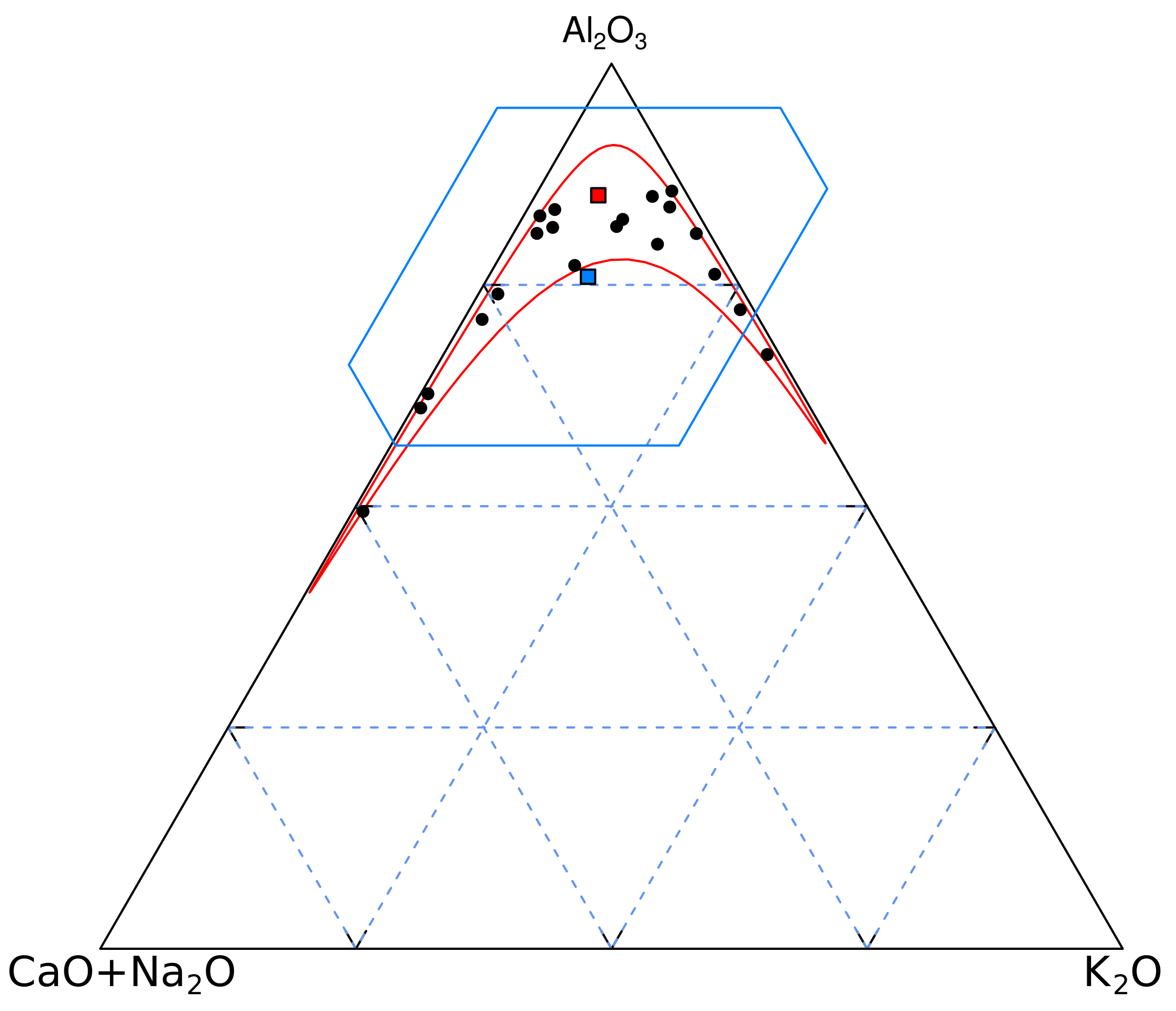
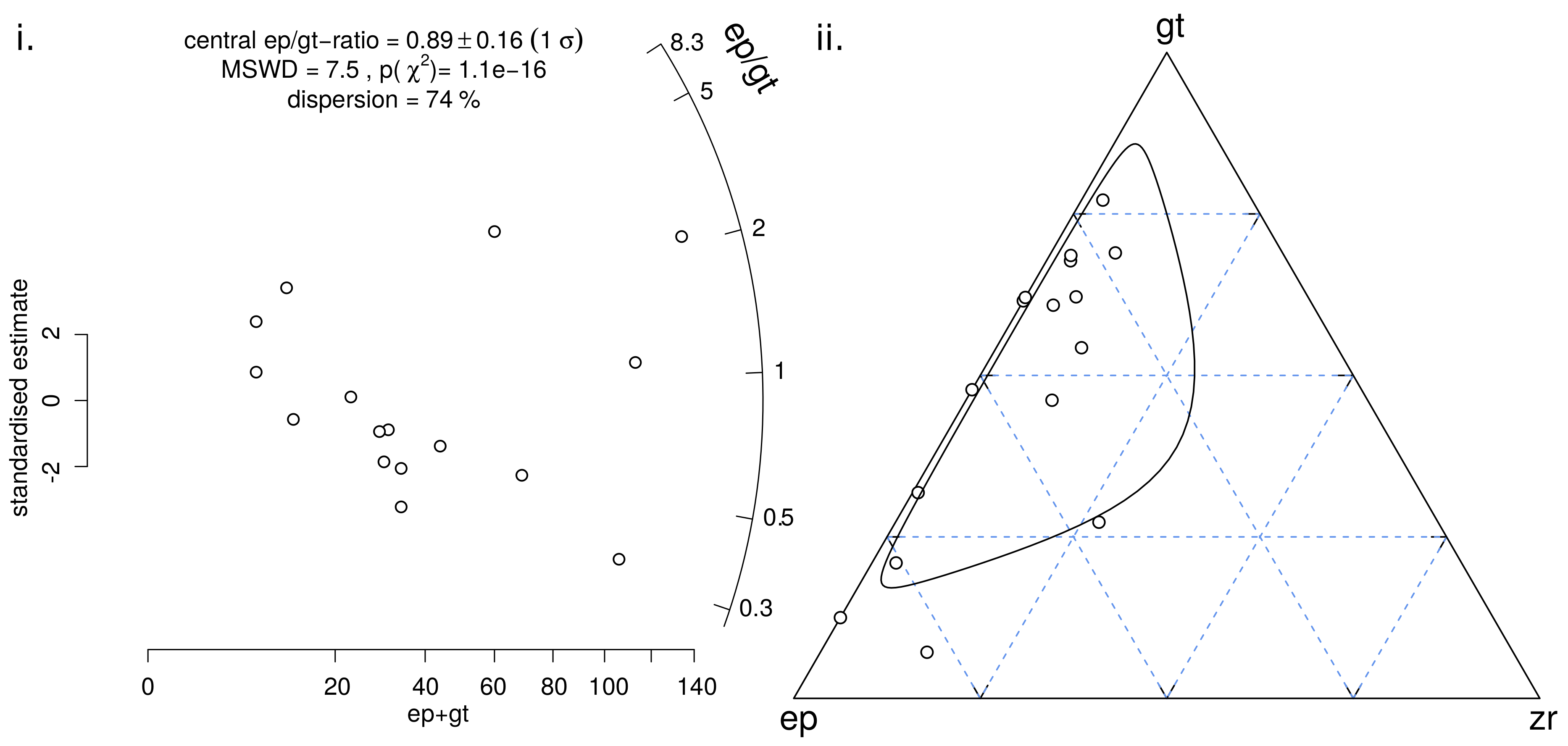
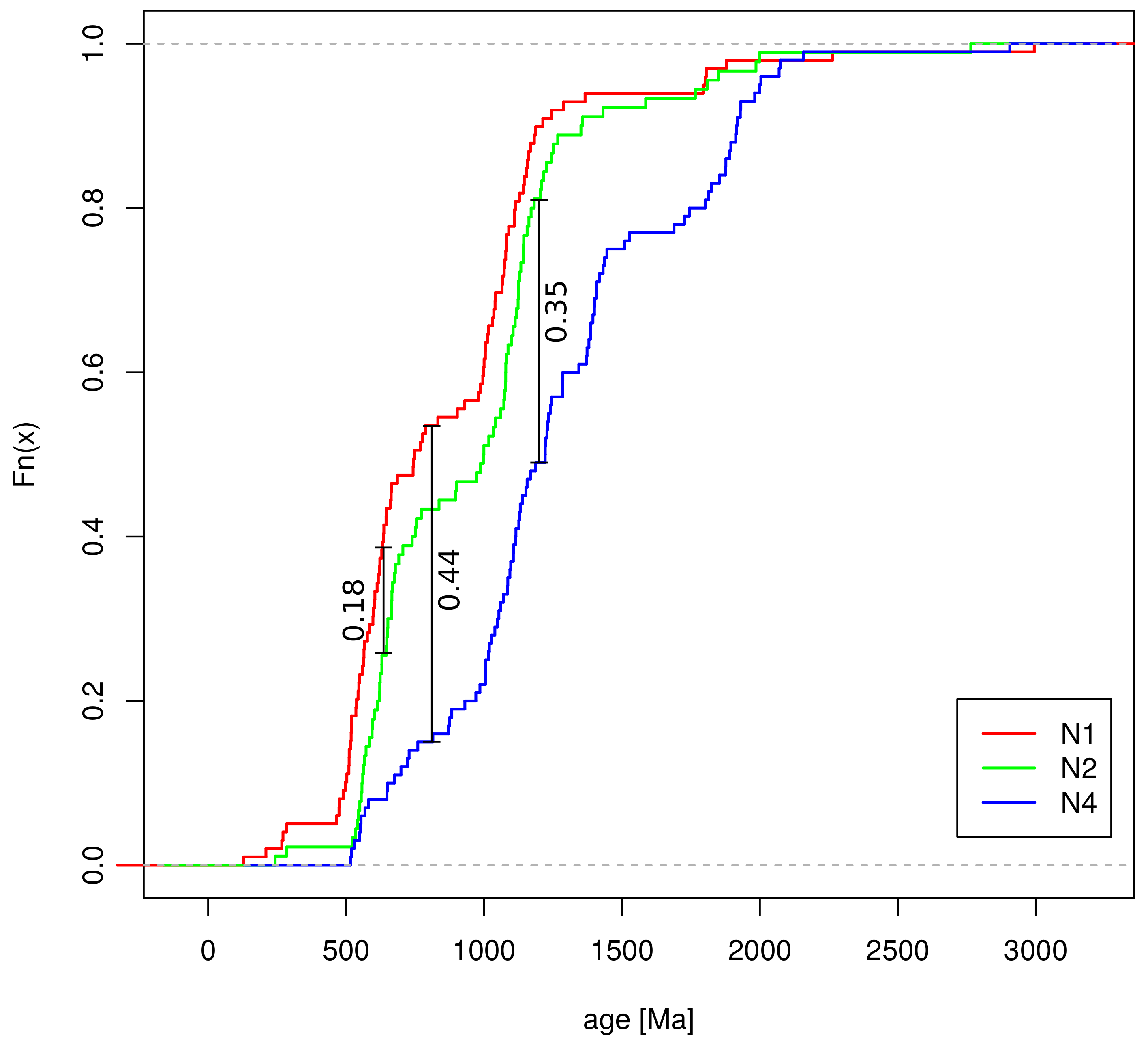
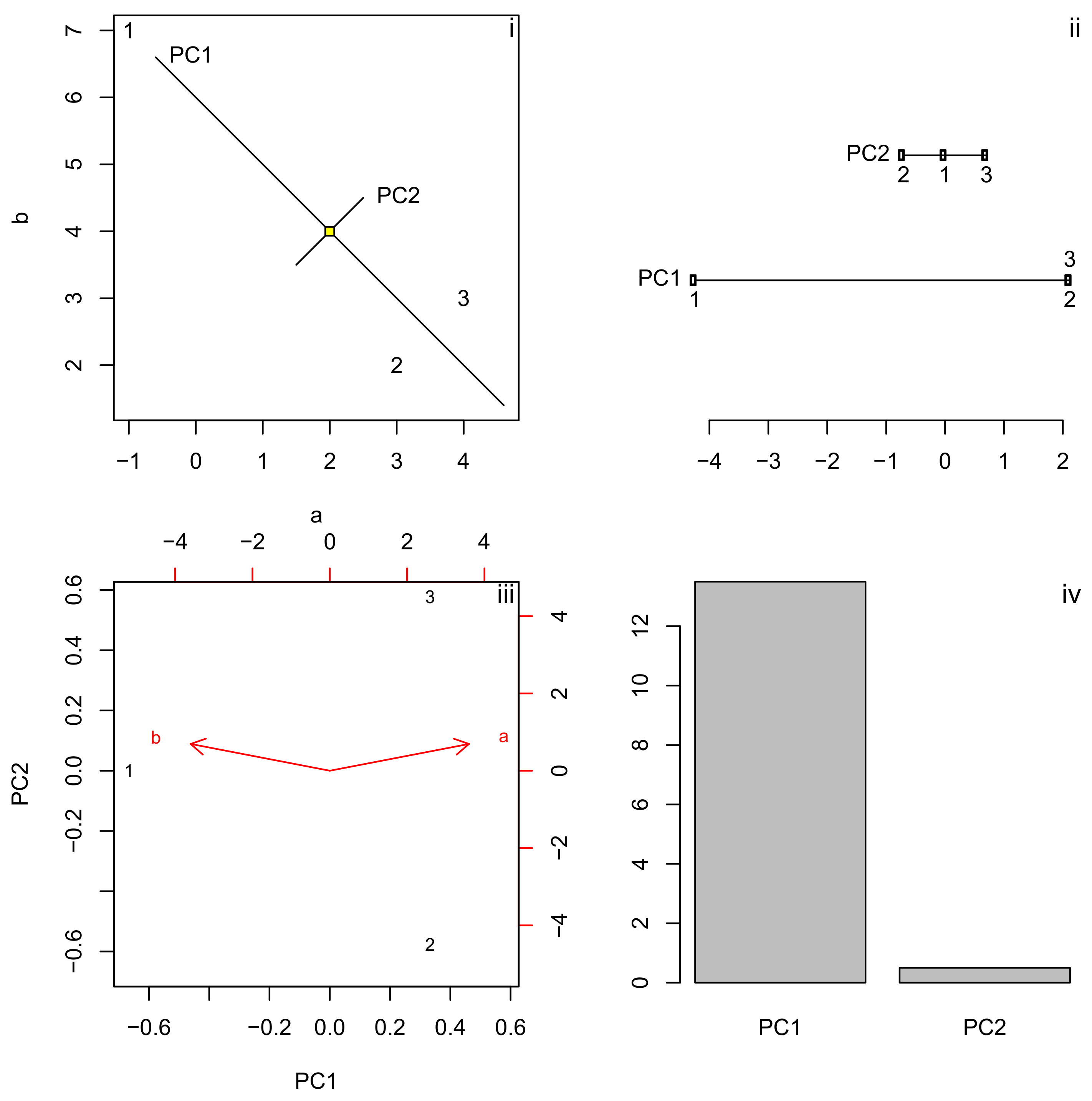
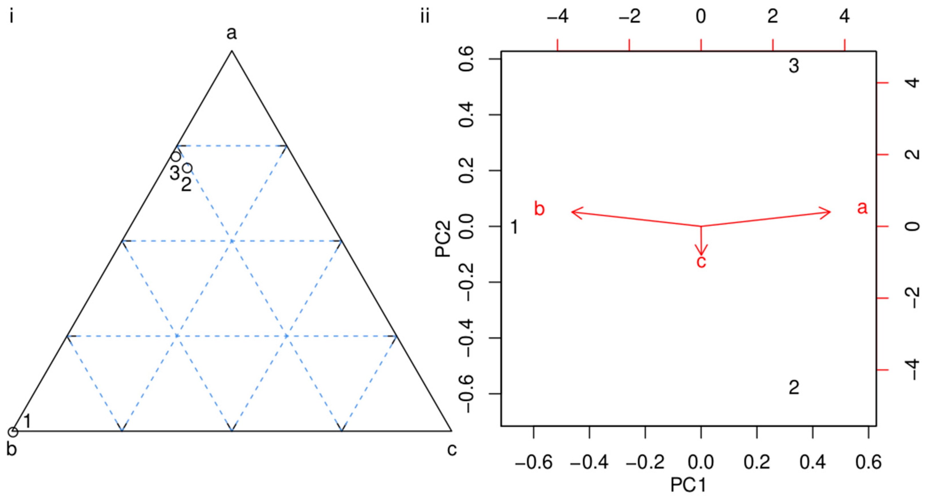
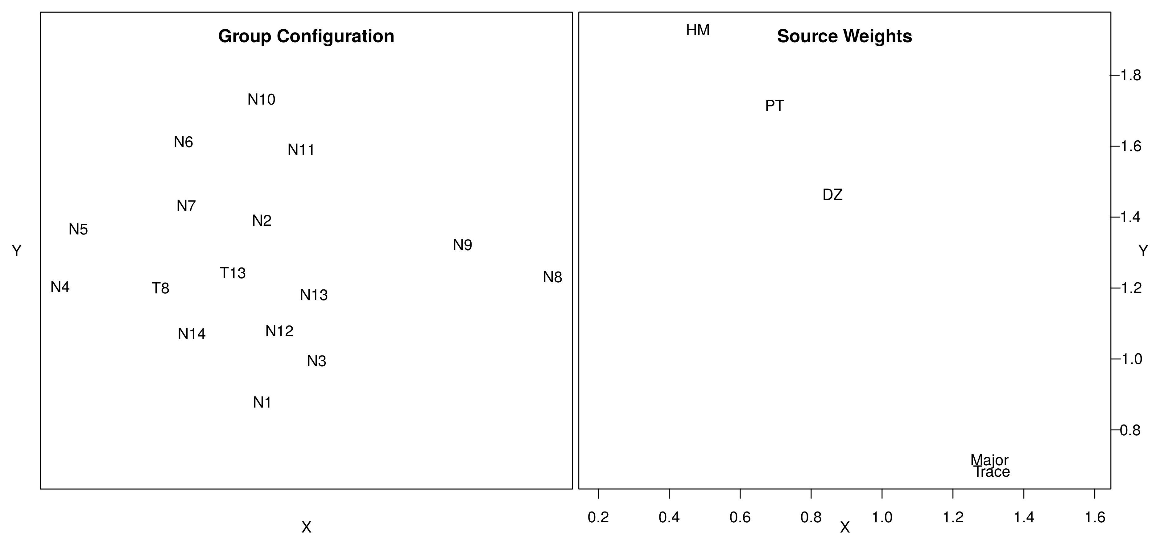
Table 1.
A summary of the three types of provenance data introduced in this paper along with a suitable dissimilarity measure and its corresponding ordination technique.
Table 1.
A summary of the three types of provenance data introduced in this paper along with a suitable dissimilarity measure and its corresponding ordination technique.
| Data Type | Dissimilarity Measure | Ordination Technique |
|---|---|---|
| compositional | Aitchison | Principal Component Analysis |
| point-counting | Chi-square | Correspondence Analysis |
| distributional | Kolmogorov–Smirnov | Multidimensional Scaling |
© 2019 by the authors. Licensee MDPI, Basel, Switzerland. This article is an open access article distributed under the terms and conditions of the Creative Commons Attribution (CC BY) license (http://creativecommons.org/licenses/by/4.0/).
Share and Cite
MDPI and ACS Style
Vermeesch, P. Exploratory Analysis of Provenance Data Using R and the Provenance Package. Minerals 2019, 9, 193. https://doi.org/10.3390/min9030193
AMA Style
Vermeesch P. Exploratory Analysis of Provenance Data Using R and the Provenance Package. Minerals. 2019; 9(3):193. https://doi.org/10.3390/min9030193
Chicago/Turabian StyleVermeesch, Pieter. 2019. "Exploratory Analysis of Provenance Data Using R and the Provenance Package" Minerals 9, no. 3: 193. https://doi.org/10.3390/min9030193
Note that from the first issue of 2016, this journal uses article numbers instead of page numbers. See further details here.