X-ray Microcomputed Tomography (µCT) for Mineral Characterization: A Review of Data Analysis Methods


Abstract
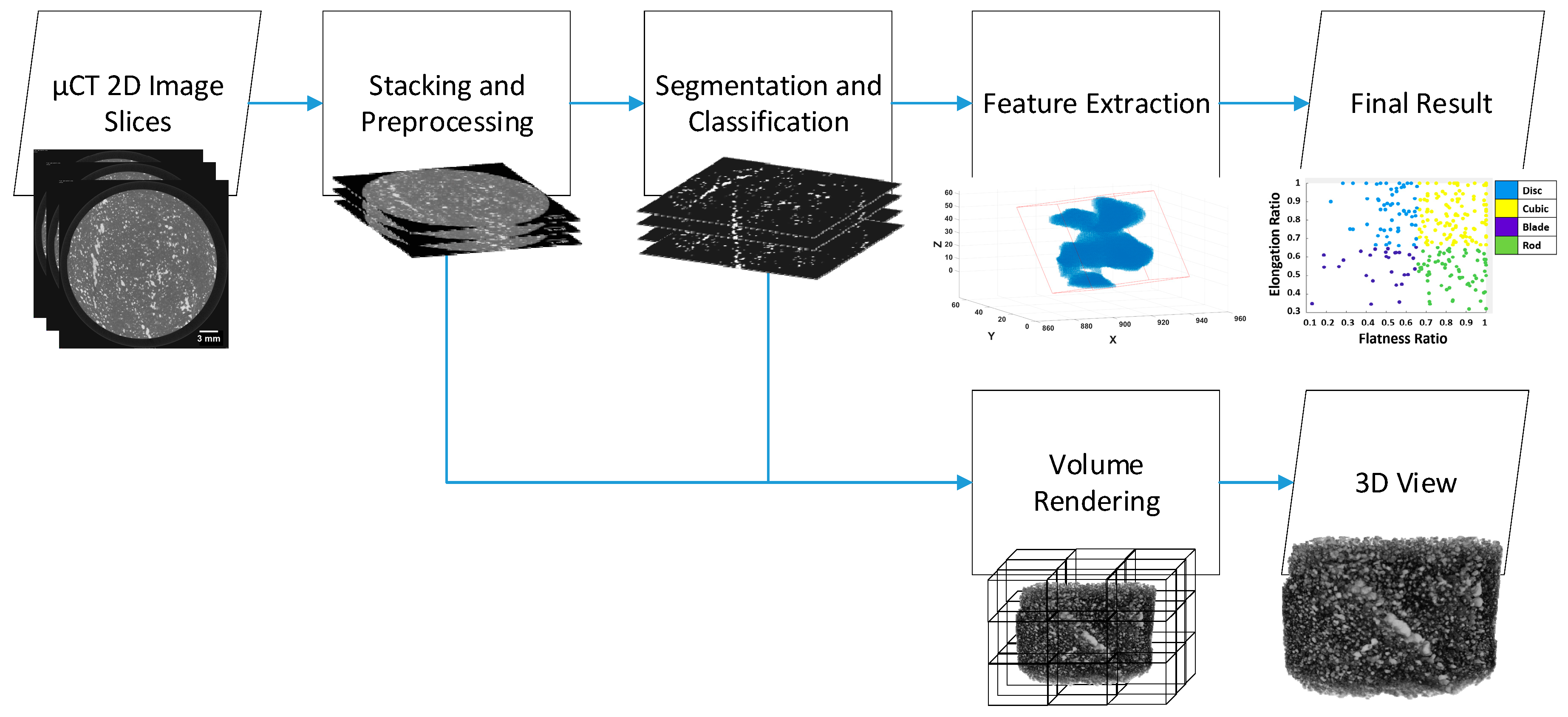
:1. Introduction
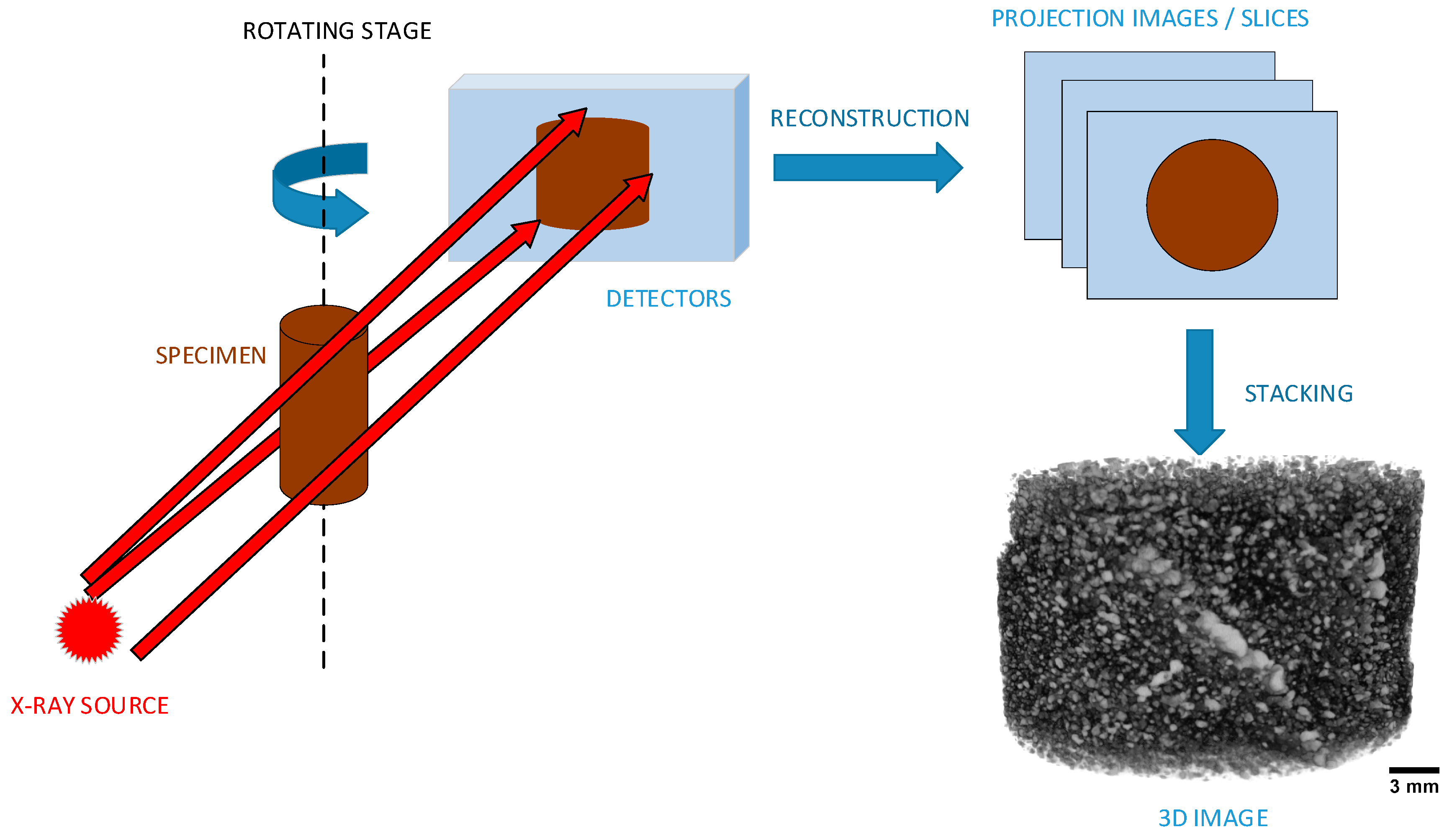
2. µCT Measurement and Data Acquisition
2.1. Measurements
2.2. Reconstruction
3. Pre-Processing
Filtering
- Denoising and blurring filters, such as Gaussian and mean filters. As the name suggests, the typical drawback of these filters is that it blurs the image, including the phase boundaries which are critical in the segmentation process. This drawback is avoided by using edge-preserving filters, such as median, non-local mean, and bilateral filters. Some researchers have applied variation of these filters in their specific cases of µCT analysis of rock samples [9,21,63].
- Sharpening and edge detection filters, such as Laplacian filters, Sobel, Canny filters, Robert, and Prewitt filters [64,65,66]. These filters are typically used in rock µCT analysis especially in crack and pore detection [8,67], watershed segmentation [68], as well as feature extraction for supervised classification [15,19,22].
4. Segmentation and Classification
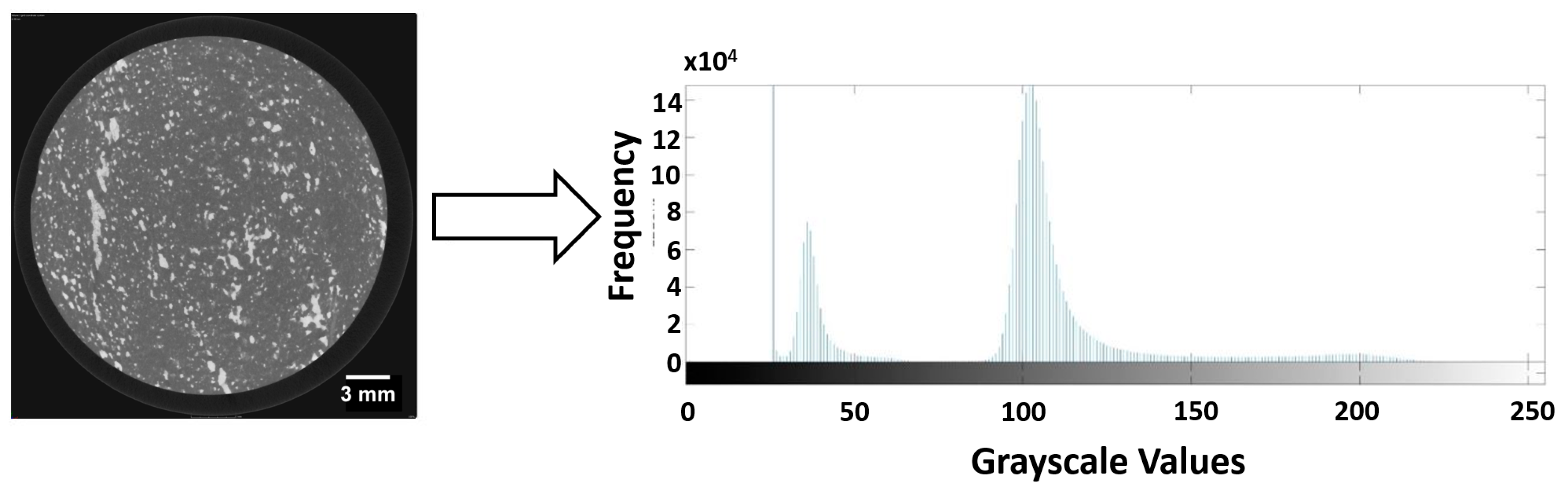
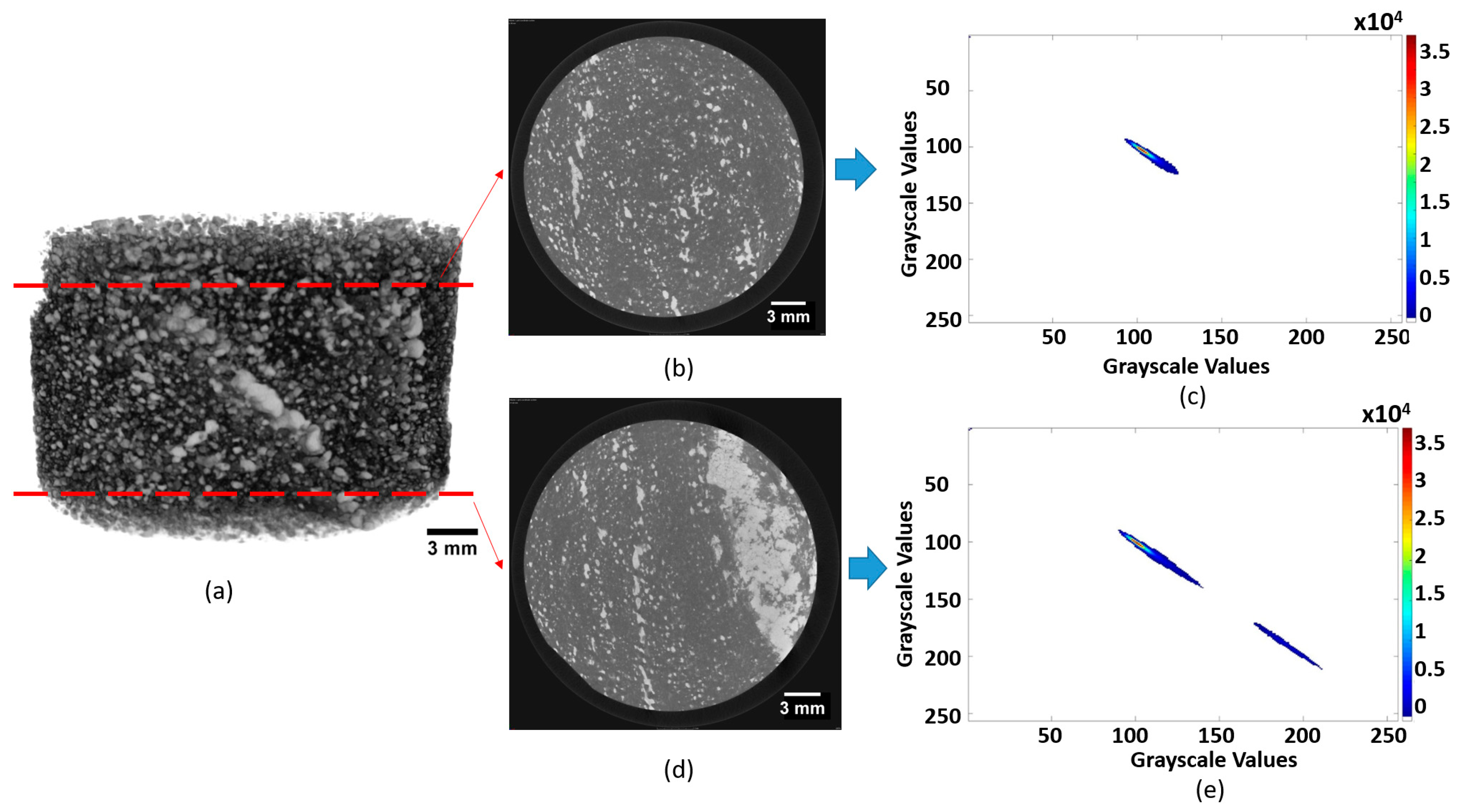
4.1. Histogram Analysis
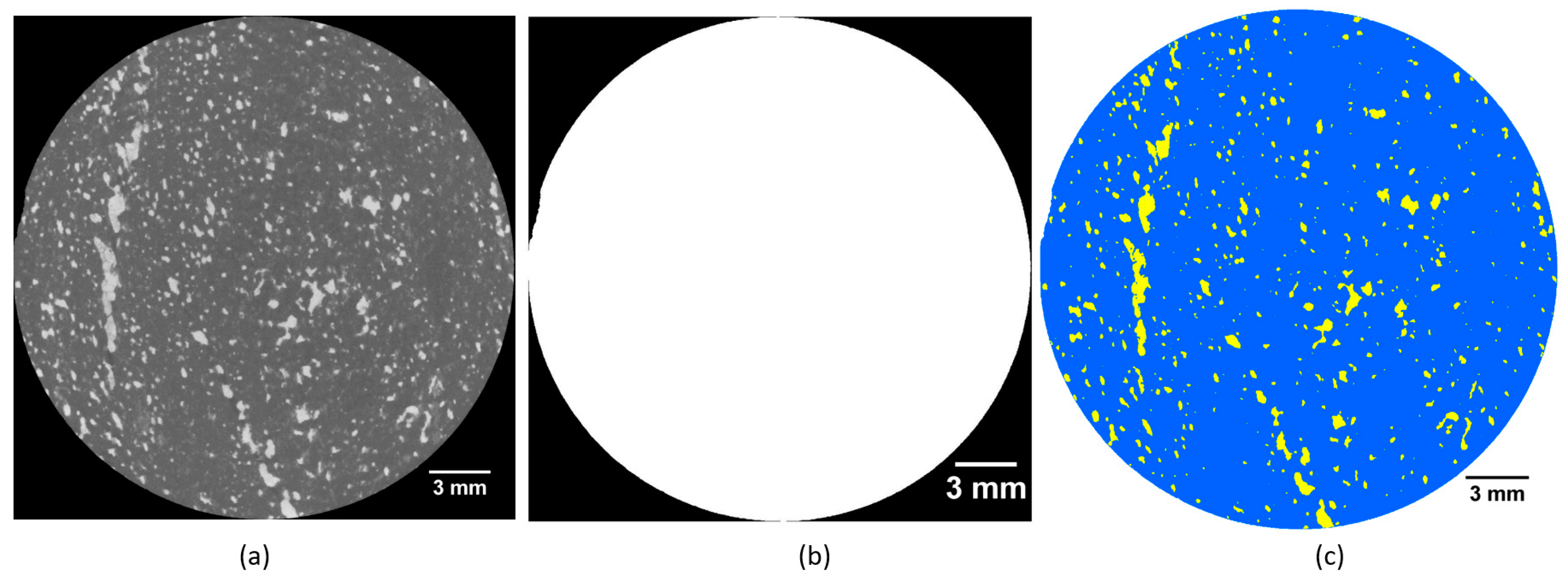
4.2. Thresholding
- Global thresholding, where the threshold value is determined from the entire image properties, for example by analyzing the whole histogram of the image as in Figure 4.
- Local thresholding, which means that instead of considering the whole image, only a certain part of the image is considered as a basis in setting a threshold value.
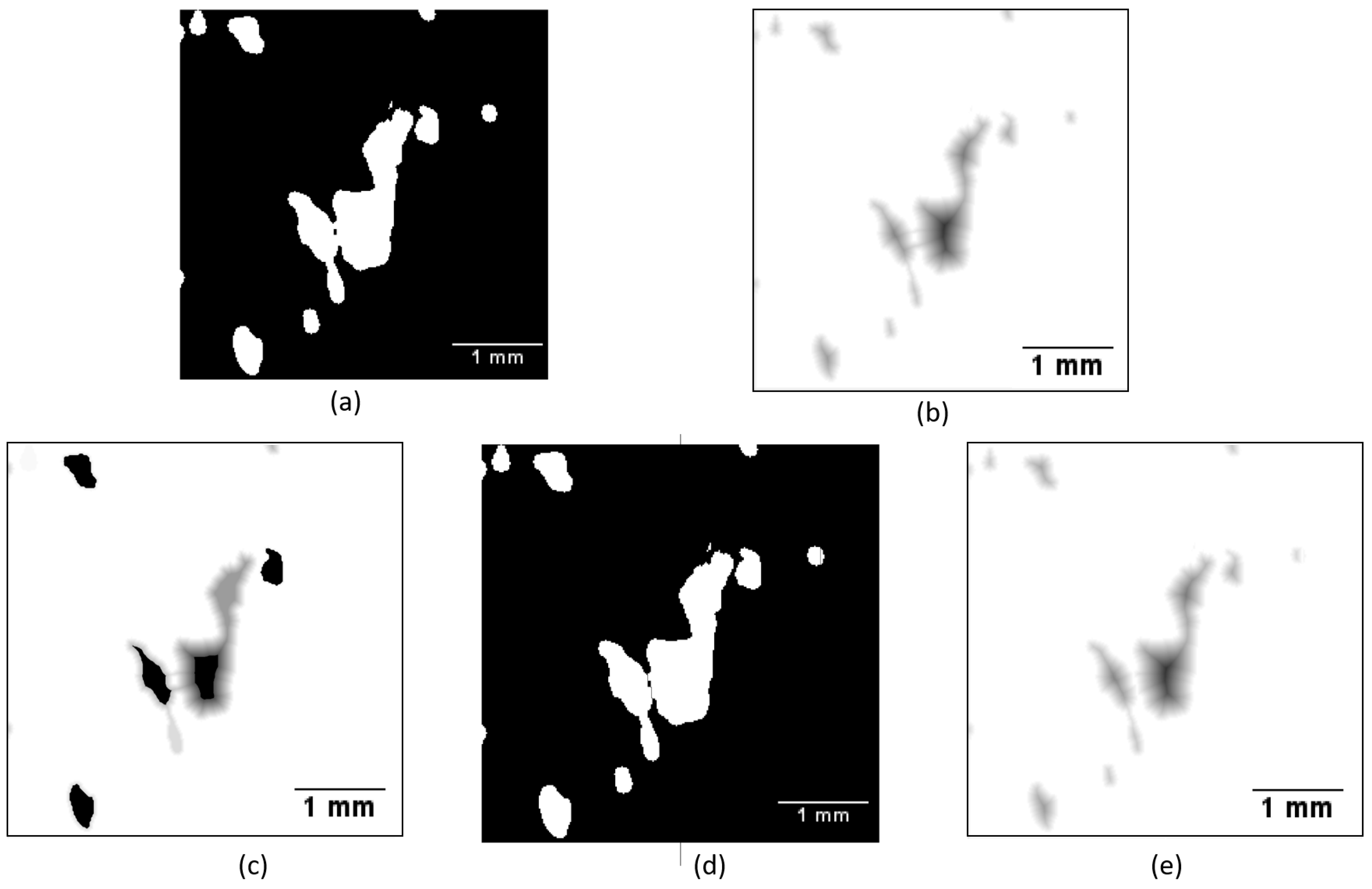
4.3. Region Growing
4.4. Unsupervised Classification
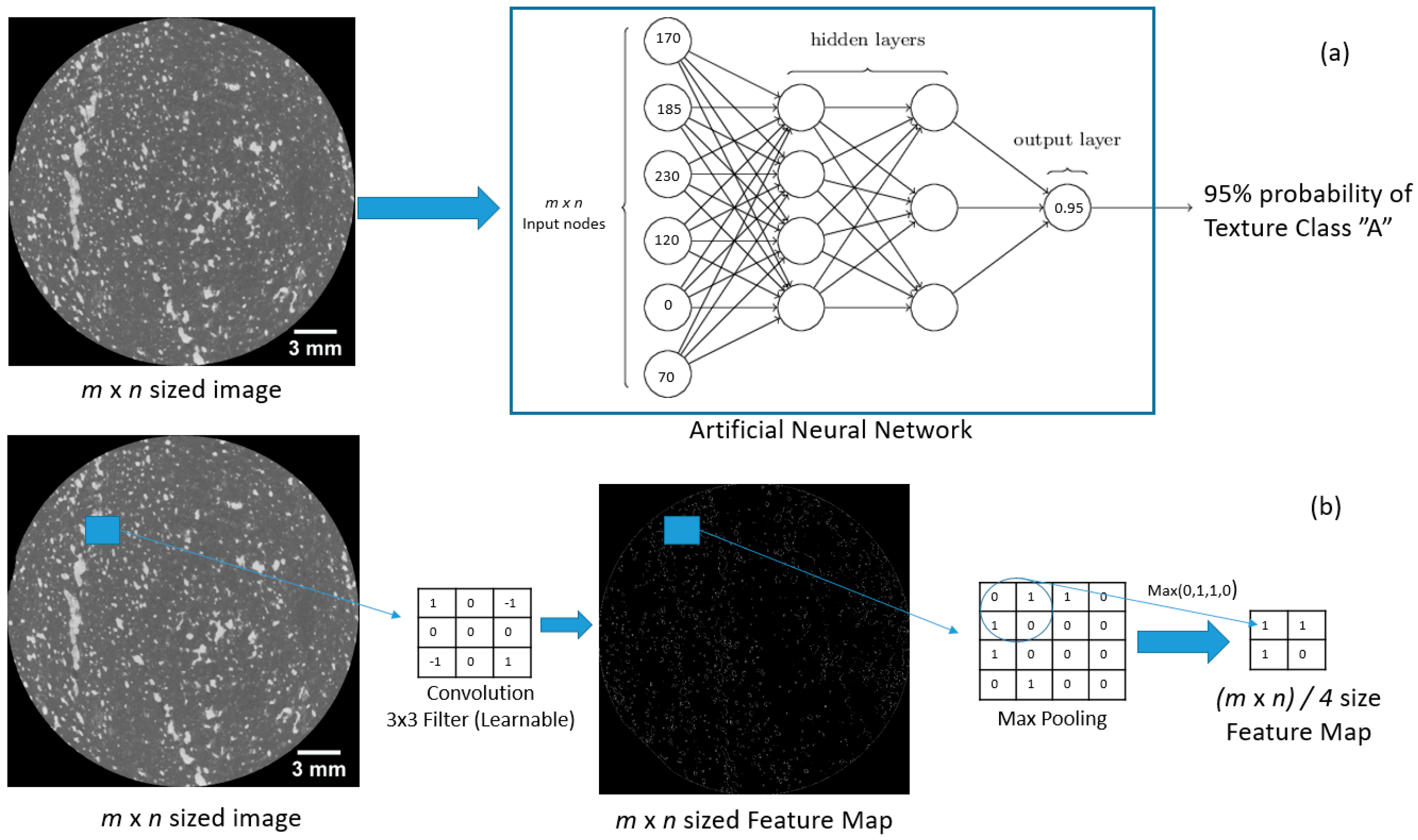
4.5. Supervised Classification
5. Feature Extraction
5.1. Distance Transformation
5.2. Mathematical Morphology
- Local orientation of textures. This is achieved by opening of the image using a line structuring element and rotating the structuring element to get directional information of the image. Such information is useful to obtain information about the isotropy of textures. It has been used in analyzing 3D datasets of fibrous networks [125].
- Global orientation of textures. While the combination of local orientations could give a good estimation on the global orientation, methods for directly determining global orientation also exist. The mean intercept length (MIL) is the most popular method to obtain this information. It generates several parallel lines in a certain direction in which the number of intercepts of the lines with the textures can be used for estimating the orientation. Such a method has been used in analyzing orientation of pores and vesicles in CT images of volcanic rocks [10].
- Skeleton of the textures. In addition to using the distance transform, the skeleton of the texture could also be obtained by eroding the features up to a certain point where its homotopy is still preserved. Such a technique is often referred to as morphological thinning.
- Shape descriptors of textures through Minkowski functionals. The Minkowski functionals are geometric measures applied to binary structures, in which for n dimensional plane, n + 1 of such functional exists. Such functionals have been applied in 3D pore analysis of soil structure [126]. These functionals are:The zeroth functional, Equation (5), calculates the mass of the object:The first functional, Equation (6), is the integral over the surface of the unit. This is simply the total surface area of the object (units: length2):The second functional, Equation (7), is the mean curvature (units: length−1) of the surface area obtained from the previous functional. Both and define the minimum and maximum radius of the curvature:The third functional, Equation (8), is the total curvature, which can be used to measure the topological properties of the object (convex, concave, or saddle).
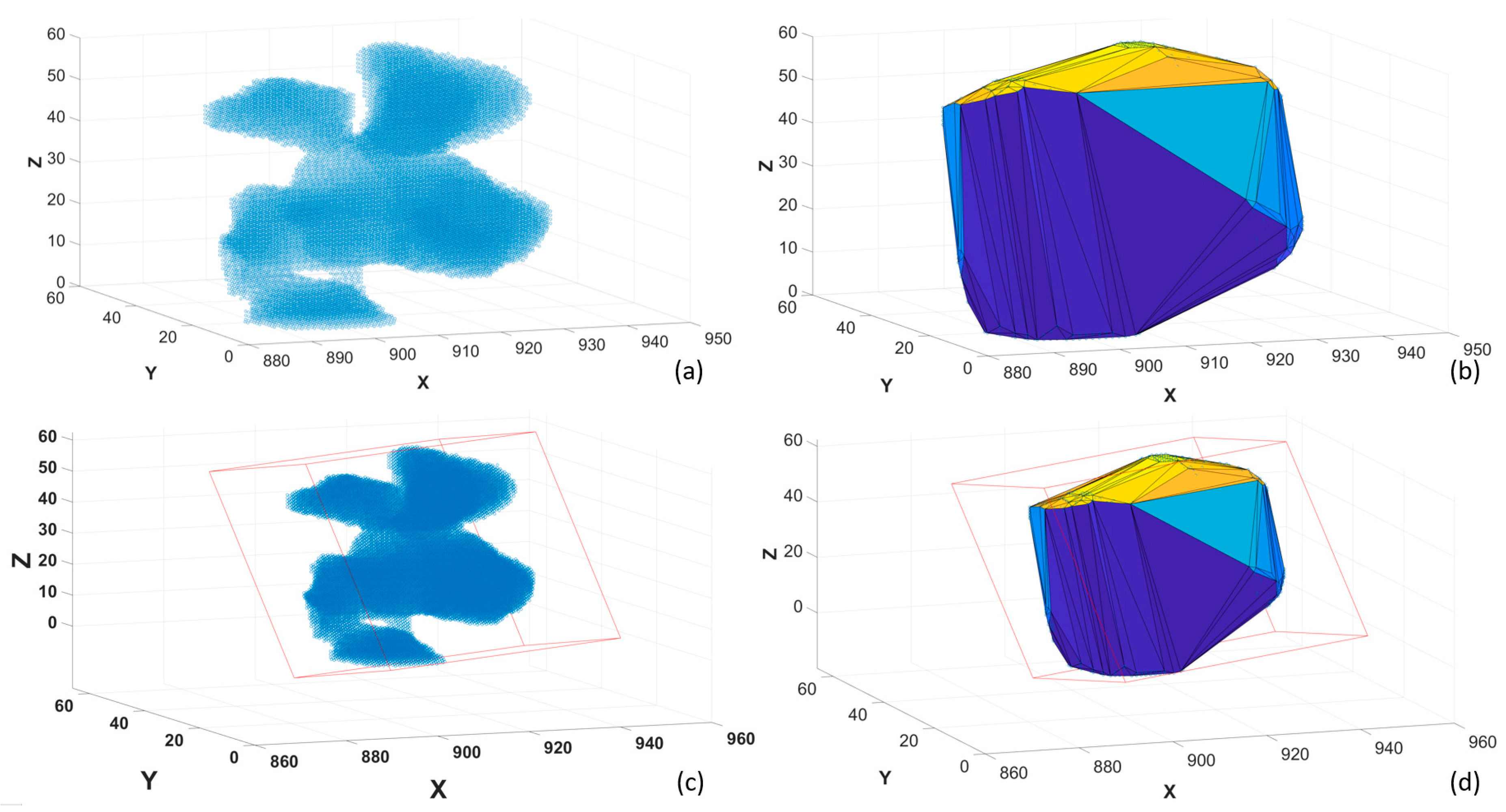
5.3. Computational Geometry
5.4. Domain Transfer Function
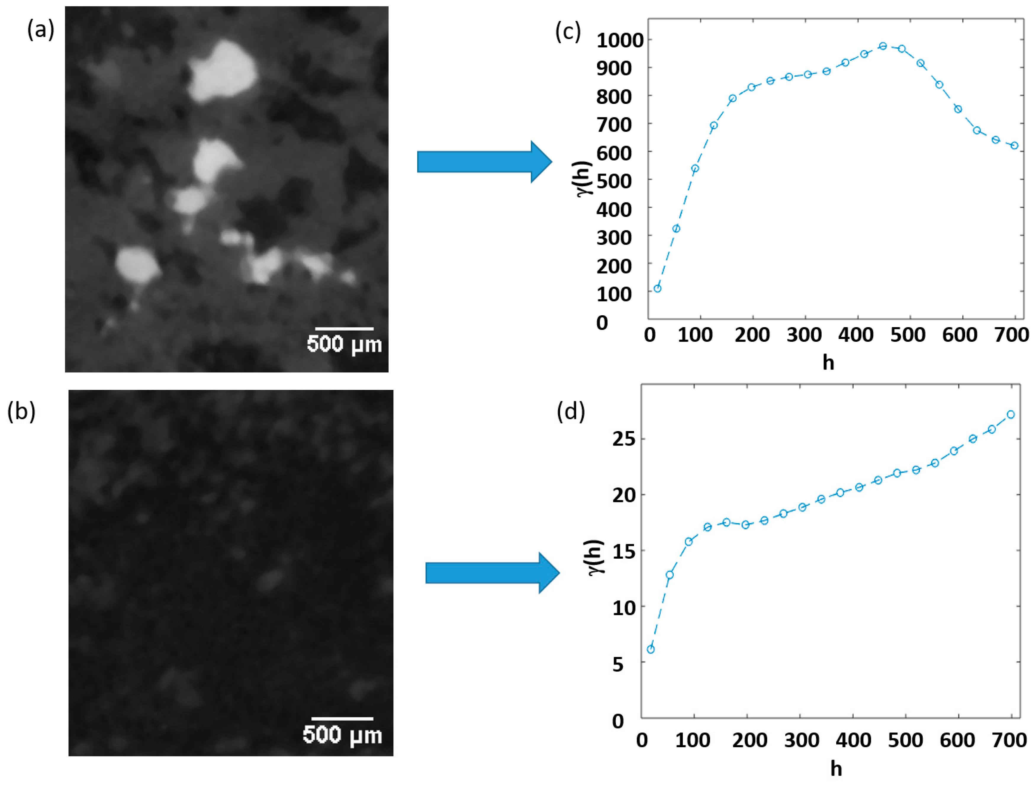
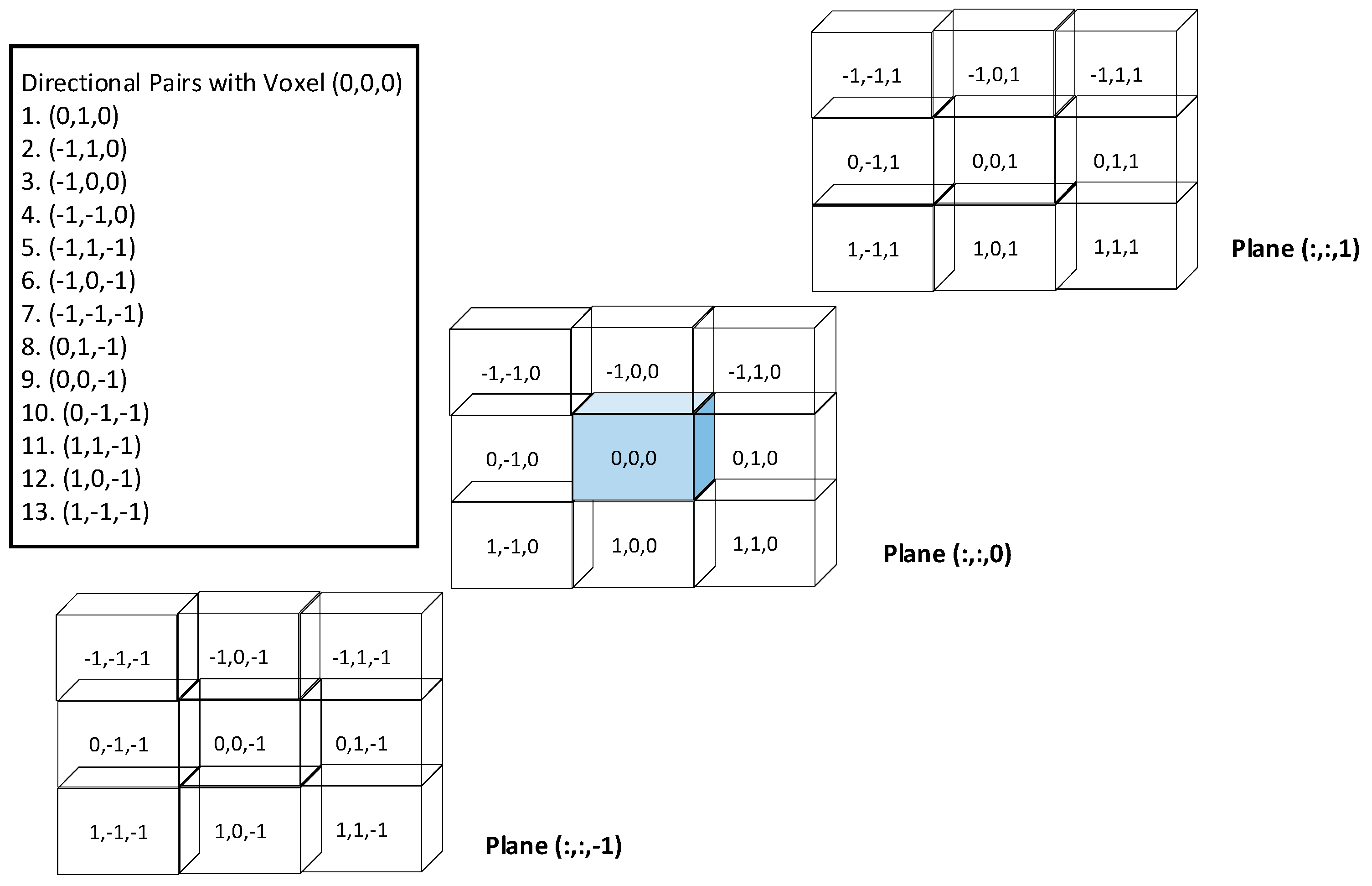
5.5. Spatial Statistics and Co-Occurrence Matrices
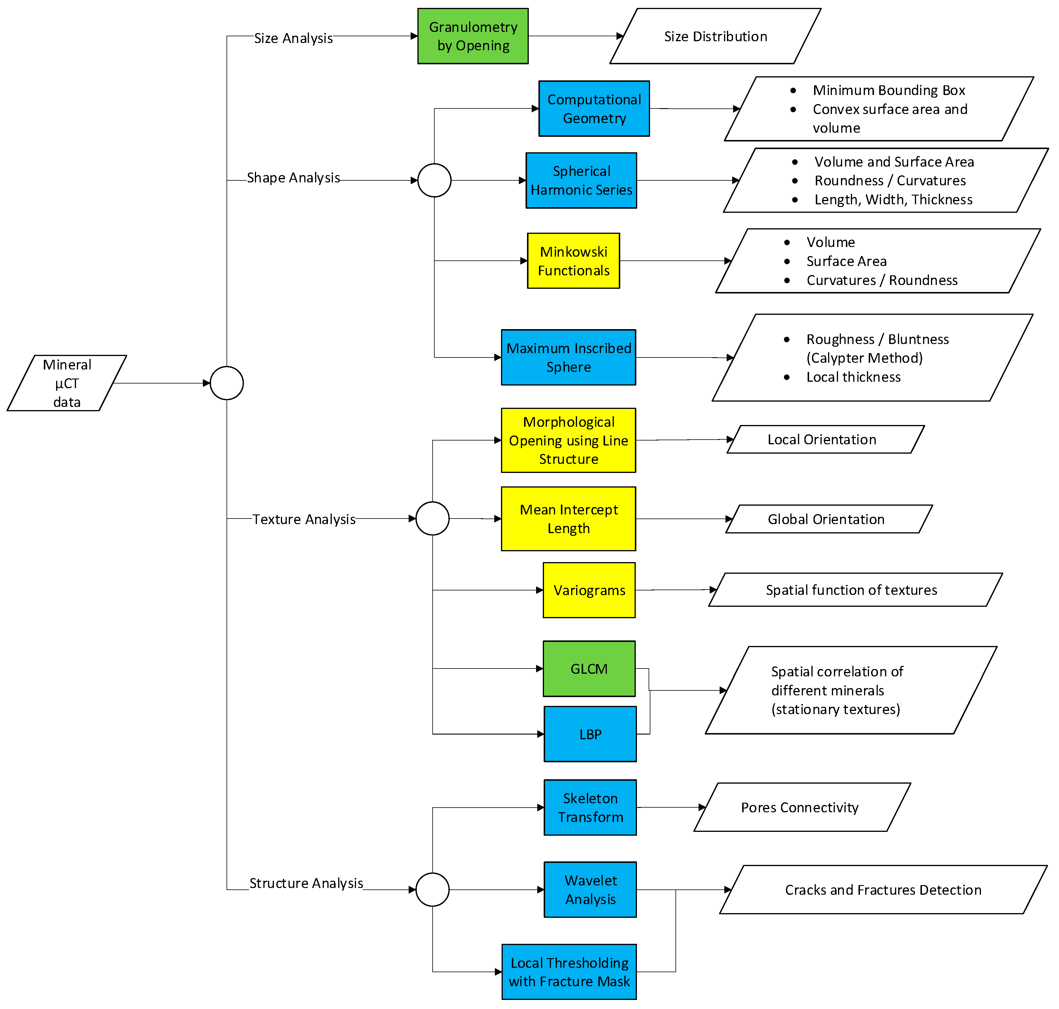
6. Summary of Data Analysis Methods
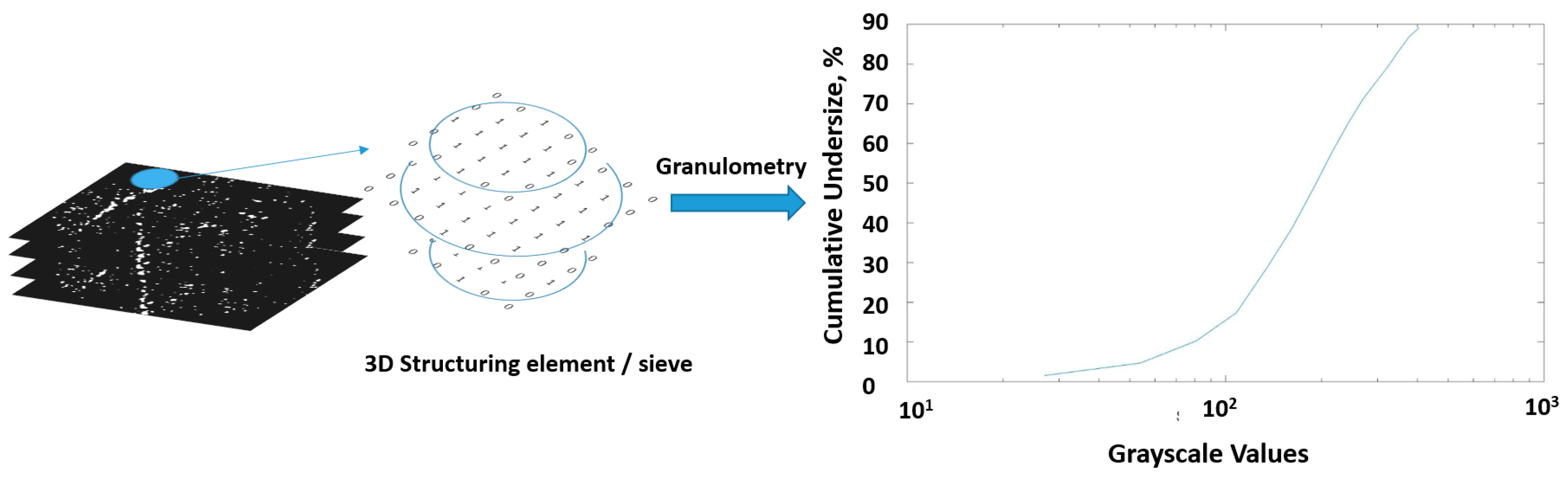
- Cases such as grain, pore, or particle size distribution analysis with µCT have been evaluated. These cases are most conveniently addressed using granulometry by opening. Improvements toward computational speed of such methods in 3D datasets have mostly been addressed by modification of the structuring element used.
- Shape analysis using µCT is more common for particulate samples; less emphasis has been put on grain shape analysis of intact ore. In these cases, computational geometry has been used, but there is always an error associated with it. Spherical harmonic series is another alternative, but it is yet more complex due to its analytical approach. Minkowski functionals allow straightforward calculations of shape descriptors, but they are limited to surface properties and topology of the shape.
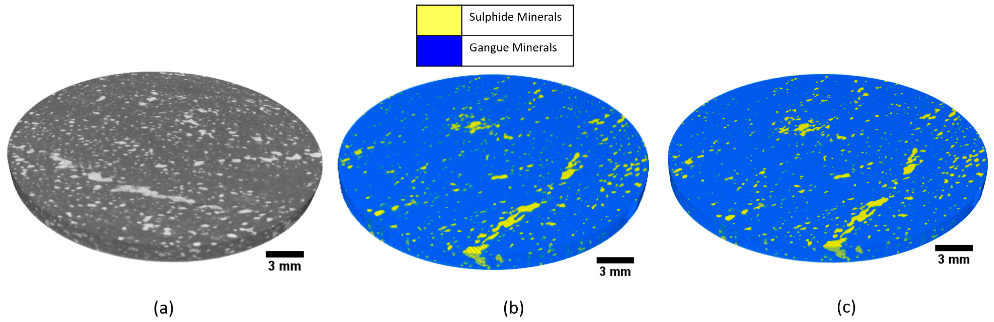
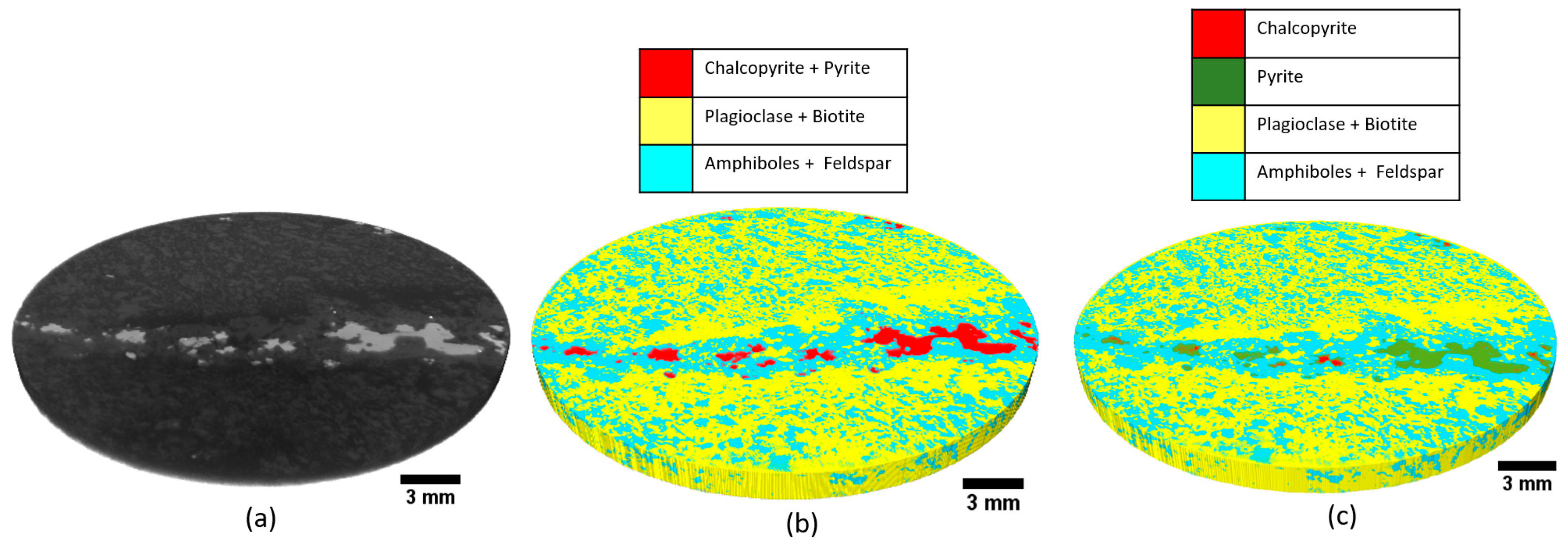
- Mineral phase segmentation can be addressed well using thresholding and unsupervised classification, provided that the target phases have enough attenuation contrasts. Additional measures must be taken when attempting to segment minerals with similar attenuations, in which such measures include dual energy µCT scanning, using lower voltage and smaller sample size, and using additional information acquired from another dataset (SEM-EDS, XRF). A more detailed summary on mineral phase segmentation with µCT is provided in Table 2.
- Stationary texture analysis in 3D has been addressed using kernel operators (such as LBP), covariance and variograms, as well as co-occurrence matrices (such as GLCM). Such techniques are potentially capable to quantify stationary textures. As these techniques rely on spatial statistics, it is restricted to textures with similar statistics across the volume (isotropic and homogenous textures). Textures with high variability across the volume might be difficult to be accurately represented. Wavelet techniques could be an alternative in texture analysis, but its current development is lagging behind, especially for 3D µCT datasets.
- Structural analysis, such as fractures, cracks, and pores, with µCT systems has also been evaluated by several researchers. The skeleton transform technique has been used in evaluating pore connectivity in a leaching column filled with ore particles. Cracks and fractures in a rock sample could be detected using wavelet analysis, or using local thresholding with a fracture mask. The latter technique has been shown to be capable of distinguishing fractures/cracks from pores.
7. Conclusions and Outlook
- In general, size, shape, and structural analysis of ore samples using µCT have been evaluated extensively by several researchers, as these parameters are best analyzed in 3D. Various data analysis methods devoting to evaluate these parameters are available with varying degree of accuracy and complexity. In relation to mineral characterization, an adequate estimation of size and shape of particulate samples could be useful in evaluating the processing behavior of such ore samples (more relevant to the field of process mineralogy and geometallurgy). Estimation on cracks and pores would be a good addition, as it could affect mineral liberation during comminution.
- It can be suggested that the bottleneck of mineral characterization with µCT lies in the mineral segmentation and mapping. Most of the µCT applications in mineral characterization are highly limited to segmentation between the major phases, such as pores, gangues, and valuable minerals (high density phases). The establishment of µCT as a rapid, standalone, and automated mineralogical analysis is challenging, as the result of this study indicates that additional information (SEM-EDS, XRF, calibration with pure minerals, dual energy) are required to effectively segment between different mineral phases in the µCT dataset. Future works should also include how to effectively combine this additional information to the µCT data processing workflow.
- Mineral texture analysis using µCT is a potential yet to be explored. Textural analysis with µCT systems is more prevalent with cases of soil, fibrous materials, as well as aggregates. In such materials the notion of texture is mostly limited to structural textures, such as morphology, surface texture (topology), and orientation. While these types of textures can be of importance in mineral characterization, the stationary textures (spatial patterns of the mineral grains) are also of interest. Various techniques have been developed to extract and quantify 3D stationary textures of ore samples. However, such techniques are currently limited to the computational expense of processing the large 3D dataset; further development is needed to optimize the computational performances of such techniques.
Author Contributions
Funding
Acknowledgments
Conflicts of Interest
References
- Cnudde, V.; Boone, M.N. High-resolution X-ray computed tomography in geosciences: A review of the current technology and applications. Earth-Sci. Rev. 2013, 123, 1–17. [Google Scholar] [CrossRef]
- Mees, F.; Swennen, R.; Van Geet, M.; Jacobs, P. Applications of X-ray computed tomography in the geosciences. Geol. Soc. Lond. Spec. Publ. 2003, 215, 1–6. [Google Scholar] [CrossRef]
- Kyle, J.R.; Ketcham, R.A. Application of high resolution X-ray computed tomography to mineral deposit origin, evaluation, and processing. Ore Geol. Rev. 2015, 65, 821–839. [Google Scholar] [CrossRef]
- Miller, J.D.; Lin, C.L.; Cortes, A.B. A review of X-ray computed tomography and its applications in mineral processing. Miner. Procesing Extr. Metall. Rev. 1990, 7, 1–18. [Google Scholar] [CrossRef]
- Lin, C.L.; Miller, J.D. 3D characterization and analysis of particle shape using X-ray microtomography (XMT). Powder Technol. 2005, 154, 61–69. [Google Scholar] [CrossRef]
- Yang, B.; Wu, A.; Narsilio, G.A.; Miao, X.; Wu, S. Use of high-resolution X-ray computed tomography and 3D image analysis to quantify mineral dissemination and pore space in oxide copper ore particles. Int. J. Miner. Metall. Mater. 2017, 24, 965–973. [Google Scholar] [CrossRef]
- Iassonov, P.; Gebrenegus, T.; Tuller, M. Segmentation of X-ray computed tomography images of porous materials: A crucial step for characterization and quantitative analysis of pore structures. Water Resour. Res. 2009, 45. [Google Scholar] [CrossRef]
- Peng, R.; Yang, Y.; Ju, Y.; Mao, L.; Yang, Y. Computation of fractal dimension of rock pores based on gray CT images. Chin. Sci. Bull. 2011, 56, 3346. [Google Scholar] [CrossRef]
- Müter, D.; Pedersen, S.; Sørensen, H.O.; Feidenhans’l, R.; Stipp, S.L.S. Improved segmentation of X-ray tomography data from porous rocks using a dual filtering approach. Comput. Geosci. 2012, 49, 131–139. [Google Scholar] [CrossRef]
- Zandomeneghi, D.; Voltolini, M.; Mancini, L.; Brun, F.; Dreossi, D.; Polacci, M. Quantitative analysis of X-ray microtomography images of geomaterials: Application to volcanic rocks. Geosphere 2010, 6, 793–804. [Google Scholar] [CrossRef]
- Lin, C.L.; Miller, J.D. Cone beam X-ray microtomography for three-dimensional liberation analysis in the 21st century. Int. J. Miner. Process. 1996, 47, 61–73. [Google Scholar] [CrossRef]
- Miller, J.D.; Lin, C.L.; Garcia, C.; Arias, H. Ultimate recovery in heap leaching operations as established from mineral exposure analysis by X-ray microtomography. Int. J. Miner. Process. 2003, 72, 331–340. [Google Scholar] [CrossRef]
- Miller, J.D.; Lin, C.-L.; Hupka, L.; Al-Wakeel, M.I. Liberation-limited grade/recovery curves from X-ray micro CT analysis of feed material for the evaluation of separation efficiency. Int. J. Miner. Process. 2009, 93, 48–53. [Google Scholar] [CrossRef]
- Reyes, F.; Lin, Q.; Cilliers, J.J.; Neethling, S.J. Quantifying mineral liberation by particle grade and surface exposure using X-ray microCT. Miner. Eng. 2018, 125, 75–82. [Google Scholar] [CrossRef]
- Wang, Y.; Lin, C.L.; Miller, J.D. Quantitative analysis of exposed grain surface area for multiphase particles using X-ray microtomography. Powder Technol. 2017, 308, 368–377. [Google Scholar] [CrossRef]
- Garcia, D.; Lin, C.L.; Miller, J.D. Quantitative analysis of grain boundary fracture in the breakage of single multiphase particles using X-ray microtomography procedures. Miner. Eng. 2009, 22, 236–243. [Google Scholar] [CrossRef]
- Ghorbani, Y.; Becker, M.; Petersen, J.; Morar, S.H.; Mainza, A.; Franzidis, J.-P. Use of X-ray computed tomography to investigate crack distribution and mineral dissemination in sphalerite ore particles. Miner. Eng. 2011, 24, 1249–1257. [Google Scholar] [CrossRef]
- Reyes, F.; Lin, Q.; Udoudo, O.; Dodds, C.; Lee, P.D.; Neethling, S.J. Calibrated X-ray micro-tomography for mineral ore quantification. Miner. Eng. 2017, 110, 122–130. [Google Scholar] [CrossRef]
- Tiu, G. Classification of Drill Core Textures for Process Simulation in Geometallurgy: Aitik Mine, New Boliden. M.Sc. Thesis, Luleå University of Technology, Luleå, Sweden, 2017. [Google Scholar]
- Andrä, H.; Combaret, N.; Dvorkin, J.; Glatt, E.; Han, J.; Kabel, M.; Keehm, Y.; Krzikalla, F.; Lee, M.; Madonna, C. Digital rock physics benchmarks—Part I: Imaging and segmentation. Comput. Geosci. 2013, 50, 25–32. [Google Scholar] [CrossRef]
- Andrä, H.; Combaret, N.; Dvorkin, J.; Glatt, E.; Han, J.; Kabel, M.; Keehm, Y.; Krzikalla, F.; Lee, M.; Madonna, C. Digital rock physics benchmarks—Part II: Computing effective properties. Comput. Geosci. 2013, 50, 33–43. [Google Scholar] [CrossRef]
- Wang, Y.; Lin, C.L.; Miller, J.D. Improved 3D image segmentation for X-ray tomographic analysis of packed particle beds. Miner. Eng. 2015, 83, 185–191. [Google Scholar] [CrossRef]
- Godel, B. High-resolution X-ray computed tomography and its application to ore deposits: From data acquisition to quantitative three-dimensional measurements with case studies from Ni-Cu-PGE deposits. Econ. Geol. 2013, 108, 2005–2019. [Google Scholar] [CrossRef]
- Jardine, M.A.; Miller, J.A.; Becker, M. Coupled X-ray computed tomography and grey level co-occurrence matrices as a method for quantification of mineralogy and texture in 3D. Comput. Geosci. 2018, 111, 105–117. [Google Scholar] [CrossRef]
- Chauhan, S.; Rühaak, W.; Khan, F.; Enzmann, F.; Mielke, P.; Kersten, M.; Sass, I. Processing of rock core microtomography images: Using seven different machine learning algorithms. Comput. Geosci. 2016, 86, 120–128. [Google Scholar] [CrossRef]
- Deng, H.; Fitts, J.P.; Peters, C.A. Quantifying fracture geometry with X-ray tomography: Technique of Iterative Local Thresholding (TILT) for 3D image segmentation. Comput. Geosci. 2016, 20, 231–244. [Google Scholar] [CrossRef]
- Alikarami, R.; Andò, E.; Gkiousas-Kapnisis, M.; Torabi, A.; Viggiani, G. Strain localisation and grain breakage in sand under shearing at high mean stress: Insights from in situ X-ray tomography. Acta Geotech. 2015, 10, 15–30. [Google Scholar] [CrossRef]
- Dobson, J.K.; Harrison, T.S.; Lin, Q.; Ní Bhreasail, A.; Fagan-Endres, A.M.; Neethling, J.S.; Lee, D.P.; Cilliers, J.J. Insights into Ferric Leaching of Low Grade Metal Sulfide-Containing ores in an Unsaturated Ore Bed Using X-ray Computed Tomography. Minerals 2017, 7, 85. [Google Scholar] [CrossRef]
- King, A.; Reischig, P.; Adrien, J.; Peetermans, S.; Ludwig, W. Polychromatic diffraction contrast tomography. Mater. Charact. 2014, 97, 1–10. [Google Scholar] [CrossRef]
- Olivo, A.; Castelli, E. X-ray phase contrast imaging: From synchrotrons to conventional sources. La Rivista Del Nuovo Cimento 2014, 37, 467–508. [Google Scholar] [CrossRef]
- Dierick, M.; Van Loo, D.; Masschaele, B.; Van den Bulcke, J.; Van Acker, J.; Van Hoorebeke, L. Recent micro-CT scanner developments at UGCT. Nucl. Instrum. Methods Phys. Res. Sect. B Beam Interact. Mater. Atoms 2014, 324, 35–40. [Google Scholar] [CrossRef]
- Lau, S.H.; Miller, J.; Lin, C.-L. 3D Mineralogy, Texture and Damage Analysis of Multiphase Mineral Particles with a High Contrast, Submicron Resolution X-ray Tomography System; Xradia Inc.: Pleasanton, CA, USA, 2012; pp. 2726–2736. [Google Scholar]
- Fusseis, F.; Xiao, X.; Schrank, C.; De Carlo, F. A brief guide to synchrotron radiation-based microtomography in (structural) geology and rock mechanics. J. Struct. Geol. 2014, 65, 1–16. [Google Scholar] [CrossRef]
- Han, I.; Demir, L.; Şahin, M. Determination of mass attenuation coefficients, effective atomic and electron numbers for some natural minerals. Radiat. Phys. Chem. 2009, 78, 760–764. [Google Scholar] [CrossRef]
- Omoumi, P.; Becce, F.; Racine, D.; Ott, J.; Andreisek, G.; Verdun, F. Dual-Energy CT: Basic Principles, Technical Approaches, and Applications in Musculoskeletal Imaging (Part 1). Semin. Musculoskelet. Radiol. 2015, 19, 431–437. [Google Scholar] [CrossRef]
- Berger, M. XCOM: Photon Cross Sections Database. 2010. Available online: http//www.nist.gov/pml/data/xcom/index.cfm (accessed on 9 March 2019).
- Bam, L.C.; Miller, J.A.; Becker, M.; Basson, I.J. X-ray computed tomography: Practical evaluation of beam hardening in iron ore samples. Miner. Eng. 2019, 131, 206–215. [Google Scholar] [CrossRef]
- Kyle, J.R.; Mote, A.S.; Ketcham, R.A. High resolution X-ray computed tomography studies of Grasberg porphyry Cu-Au ores, Papua, Indonesia. Miner. Depos. 2008, 5, 519–532. [Google Scholar] [CrossRef]
- Van Geet, M.; Swennen, R.; Wevers, M. Quantitative analysis of reservoir rocks by microfocus X-ray computerised tomography. Sediment. Geol. 2000, 132, 25–36. [Google Scholar] [CrossRef]
- Van Geet, M.; Volckaert, G.; Roels, S. The use of microfocus X-ray computed tomography in characterising the hydration of a clay pellet/powder mixture. Appl. Clay Sci. 2005, 29, 73–87. [Google Scholar] [CrossRef]
- Lai, P.; Moulton, K.; Krevor, S. Pore-scale heterogeneity in the mineral distribution and reactive surface area of porous rocks. Chem. Geol. 2015, 411, 260–273. [Google Scholar] [CrossRef]
- Barnes, S.J.; Le Vaillant, M.; Lightfoot, P.C. Textural development in sulfide-matrix ore breccias in the Voisey’s Bay Ni-Cu-Co deposit, Labrador, Canada. Ore Geol. Rev. 2017, 90, 414–438. [Google Scholar] [CrossRef]
- Ducheyne, P.; Healy, K.; Hutmacher, D.W.; Grainger, D.W.; Kirkpatrick, C.J. Comprehensive Biomaterials II; Elsevier: Amsterdam, The Netherlands, 2017; ISBN 0081006926. [Google Scholar]
- Kastner, J.; Harrer, B.; Requena, G.; Brunke, O. A comparative study of high resolution cone beam X-ray tomography and synchrotron tomography applied to Fe- and Al-alloys. NDT E Int. 2010, 43, 599–605. [Google Scholar] [CrossRef]
- Boas, F.E.; Fleischmann, D. CT artifacts: Causes and reduction techniques. Imaging Med. 2012, 4. [Google Scholar] [CrossRef]
- Schwarz, T. Artifacts in CT. In Veterinary Computed Tomography; John Wiley & Sons, Ltd.: Hoboken, NJ, USA, 2011; pp. 35–55. ISBN 9781118785676. [Google Scholar]
- Wildenschild, D.; Vaz, C.M.P.; Rivers, M.L.; Rikard, D.; Christensen, B.S.B. Using X-ray computed tomography in hydrology: Systems, resolutions, and limitations. J. Hydrol. 2002, 267, 285–297. [Google Scholar] [CrossRef]
- Suuronen, J.-P.; Sayab, M. 3D nanopetrography and chemical imaging of datable zircons by synchrotron multimodal X-ray tomography. Sci. Rep. 2018, 8, 4747. [Google Scholar] [CrossRef] [PubMed]
- Sun, J.; Yu, T.; Xu, C.; Ludwig, W.; Zhang, Y. 3D characterization of partially recrystallized Al using high resolution diffraction contrast tomography. Scr. Mater. 2018, 157, 72–75. [Google Scholar] [CrossRef]
- Kikuchi, S.; Nonaka, K.; Asakawa, N.; Shiozawa, D.; Nakai, Y. Change of misorientation of individual grains in fatigue of polycrystalline alloys by diffraction contrast tomography using ultrabright synchrotron radiation. Procedia Struct. Integr. 2017, 3, 402–410. [Google Scholar] [CrossRef]
- Herbig, M.; King, A.; Reischig, P.; Proudhon, H.; Lauridsen, E.M.; Marrow, J.; Buffière, J.-Y.; Ludwig, W. 3-D growth of a short fatigue crack within a polycrystalline microstructure studied using combined diffraction and phase-contrast X-ray tomography. Acta Mater. 2011, 59, 590–601. [Google Scholar] [CrossRef]
- King, A.; Herbig, M.; Ludwig, W.; Reischig, P.; Lauridsen, E.M.; Marrow, T.; Buffière, J.Y. Non-destructive analysis of micro texture and grain boundary character from X-ray diffraction contrast tomography. Nucl. Instrum. Methods Phys. Res. Sect. B Beam Interact. Mater. Atoms 2010, 268, 291–296. [Google Scholar] [CrossRef]
- Toda, H.; Takijiri, A.; Azuma, M.; Yabu, S.; Hayashi, K.; Seo, D.; Kobayashi, M.; Hirayama, K.; Takeuchi, A.; Uesugi, K. Damage micromechanisms in dual-phase steel investigated with combined phase- and absorption-contrast tomography. Acta Mater. 2017, 126, 401–412. [Google Scholar] [CrossRef]
- Artioli, G.; Cerulli, T.; Cruciani, G.; Dalconi, M.C.; Ferrari, G.; Parisatto, M.; Rack, A.; Tucoulou, R. X-ray diffraction microtomography (XRD-CT), a novel tool for non-invasive mapping of phase development in cement materials. Anal. Bioanal. Chem. 2010, 397, 2131–2136. [Google Scholar] [CrossRef]
- Takahashi, H.; Sugiyama, T. Application of non-destructive integrated CT-XRD method to investigate alteration of cementitious materials subjected to high temperature and pure water. Constr. Build. Mater. 2019, 203, 579–588. [Google Scholar] [CrossRef]
- Laforce, B.; Masschaele, B.; Boone, M.N.; Schaubroeck, D.; Dierick, M.; Vekemans, B.; Walgraeve, C.; Janssen, C.; Cnudde, V.; Van Hoorebeke, L.; et al. Integrated Three-Dimensional Microanalysis Combining X-Ray Microtomography and X-Ray Fluorescence Methodologies. Anal. Chem. 2017, 89, 10617–10624. [Google Scholar] [CrossRef] [PubMed]
- Viermetz, M.; Birnbacher, L.; Willner, M.; Achterhold, K.; Pfeiffer, F.; Herzen, J. High resolution laboratory grating-based X-ray phase-contrast CT. Sci. Rep. 2018, 8, 15884. [Google Scholar] [CrossRef] [PubMed]
- Dudgeon, D.E.; Mersereau, R.M. Multidimensional Digital Signal Processing Prentice-Hall Signal Processing Series; Prentice-Hall: Englewood Cliffs, NJ, USA, 1984. [Google Scholar]
- Feldkamp, L.A.; Davis, L.C.; Kress, J.W. Practical cone-beam algorithm. J. Opt. Soc. Am. A 1984, 1, 612–619. [Google Scholar] [CrossRef]
- Lin, Q.; Andrew, M.; Thompson, W.; Blunt, M.J.; Bijeljic, B. Optimization of image quality and acquisition time for lab-based X-ray microtomography using an iterative reconstruction algorithm. Adv. Water Resour. 2018, 115, 112–124. [Google Scholar] [CrossRef]
- Zhuge, X.; Palenstijn, W.J.; Batenburg, K.J. TVR-DART: A More Robust Algorithm for Discrete Tomography From Limited Projection Data With Automated Gray Value Estimation. IEEE Trans. Image Process. 2016, 25, 455–468. [Google Scholar] [CrossRef]
- Myers, G.R.; Kingston, A.M.; Varslot, T.K.; Turner, M.L.; Sheppard, A.P. Dynamic tomography with a priori information. Appl. Opt. 2011, 50, 3685–3690. [Google Scholar] [CrossRef] [PubMed]
- Brabant, L.; Vlassenbroeck, J.; De Witte, Y.; Cnudde, V.; Boone, M.N.; Dewanckele, J.; Van Hoorebeke, L. Three-Dimensional Analysis of High-Resolution X-Ray Computed Tomography Data with Morpho+. Microsc. Microanal. 2011, 17, 252–263. [Google Scholar] [CrossRef] [PubMed]
- Canny, J. A computational approach to edge detection. IEEE Trans. Pattern Anal. Mach. Intell. 1986, 679–698. [Google Scholar] [CrossRef]
- Prewitt, J.M.S. Object enhancement and extraction. Pict. Process. Psychopictorics 1970, 10, 15–19. [Google Scholar]
- Sobel, I. An Isotropic 3x3 Image Gradient Operator. 2014. Available online: https://www.researchgate.net/publication/239398674_An_Isotropic_3x3_Image_Gradient_Operator (accessed on 14 March 2019).
- Chun, B.; Xiaoyue, L. The edge detection technology of CT image for study the growth of rock crack. In Proceedings of the 2009 ISECS International Colloquium on Computing, Communication, Control, and Management, Sanya, China, 8–9 August 2009; Volume 4, pp. 286–288. [Google Scholar]
- Schlüter, S.; Sheppard, A.; Brown, K.; Wildenschild, D. Image processing of multiphase images obtained via X-ray microtomography: A review. Water Resour. Res. 2014, 50, 3615–3639. [Google Scholar] [CrossRef]
- Martínez-Martínez, J.; Benavente, D.; Del Cura, M.A.G. Petrographic quantification of brecciated rocks by image analysis. Application to the interpretation of elastic wave velocities. Eng. Geol. 2007, 90, 41–54. [Google Scholar] [CrossRef]
- Kaur, D.; Kaur, Y. Various Image Segmentation Techniques: A Review. Int. J. Comput. Sci. Mob. Comput. 2014, 3, 809–814. [Google Scholar]
- Yogamangalam, R.; Karthikeyan, B. Segmentation techniques comparison in image processing. Int. J. Eng. Technol. 2013, 5, 307–313. [Google Scholar]
- Zaitoun, N.M.; Aqel, M.J. Survey on image segmentation techniques. Procedia Comput. Sci. 2015, 65, 797–806. [Google Scholar] [CrossRef]
- Sezgin, M.; Sankur, B. Survey over image thresholding techniques and quantitative performance evaluation. J. Electron. Imaging 2004, 13, 146–166. [Google Scholar]
- Kaczmarczyk, J.; Dohnalik, M.; Zalewska, J.; Cnudde, V. The Interpretation of X-ray Computed Microtomography Images of Rocks as an Application of Volume Image Processing and Analysis. 2010. Available online: https://biblio.ugent.be/publication/1020385/file/1020401.pdf (accessed on 14 March 2019).
- Otsu, N. A threshold selection method from gray-level histograms. IEEE Trans. Syst. Man. Cybern. 1979, 9, 62–66. [Google Scholar] [CrossRef]
- Lin, Q.; Barker, D.J.; Dobson, K.J.; Lee, P.D.; Neethling, S.J. Modelling particle scale leach kinetics based on X-ray computed micro-tomography images. Hydrometallurgy 2016, 162, 25–36. [Google Scholar] [CrossRef]
- Lin, Q.; Neethling, S.J.; Dobson, K.J.; Courtois, L.; Lee, P.D. Quantifying and minimising systematic and random errors in X-ray micro-tomography based volume measurements. Comput. Geosci. 2015, 77, 1–7. [Google Scholar] [CrossRef]
- Fan, S.-K.S.; Lin, Y. A multi-level thresholding approach using a hybrid optimal estimation algorithm. Pattern Recognit. Lett. 2007, 28, 662–669. [Google Scholar] [CrossRef]
- Huang, D.-Y.; Wang, C.-H. Optimal multi-level thresholding using a two-stage Otsu optimization approach. Pattern Recognit. Lett. 2009, 30, 275–284. [Google Scholar] [CrossRef]
- Kapur, J.N.; Sahoo, P.K.; Wong, A.K.C. A new method for gray-level picture thresholding using the entropy of the histogram. Comput. Vis. Graphics Image Process. 1985, 29, 273–285. [Google Scholar] [CrossRef]
- Gonzalez, R.C.; Woods, R.E. Digital Image Processing; Prentice Hall: Upper Saddle River, NJ, USA, 2002. [Google Scholar]
- Ketcham, R.A. Computational methods for quantitative analysis of three-dimensional features in geological specimens. Geosphere 2005, 1, 32–41. [Google Scholar] [CrossRef]
- Meyer, F.; Beucher, S. Morphological segmentation. J. Vis. Commun. Image Represent. 1990, 1, 21–46. [Google Scholar] [CrossRef]
- Wang, D.; Vallotton, P. Improved marker-controlled watershed segmentation with local boundary priors. In Proceedings of the 2010 25th International Conference of Image and Vision Computing New Zealand, Queenstown, New Zealand, 8–9 November 2010; pp. 1–6. [Google Scholar]
- Vincent, L.; Soille, P. Watersheds in digital spaces: An efficient algorithm based on immersion simulations. IEEE Trans. Pattern Anal. Mach. Intell. 1991, 6, 583–598. [Google Scholar] [CrossRef]
- Weickert, J. Efficient image segmentation using partial differential equations and morphology. Pattern Recognit. 2001, 34, 1813–1824. [Google Scholar] [CrossRef]
- Jung, C.R.; Scharcanski, J. Robust watershed segmentation using wavelets. Image Vis. Comput. 2005, 23, 661–669. [Google Scholar] [CrossRef]
- Belaid, L.J.; Mourou, W. Image segmentation: A watershed transformation algorithm. Image Anal. Stereol. 2011, 28, 93–102. [Google Scholar] [CrossRef]
- Lin, C.L.; Miller, J.D. Advances in X-ray computed tomography (CT) for improved coal washability analysis. In Proceedings of the 16th International Coal Preparation Congress, ICPC 2010, Lexington, KY, USA, 25–30 April 2010. [Google Scholar]
- Lin, C.L.; Videla, A.R.; Yu, Q.; Miller, J.D. Characterization and analysis of Porous, Brittle solid structures by X-ray micro computed tomography. JOM 2010, 62, 86–89. [Google Scholar] [CrossRef]
- Kong, D.; Fonseca, J. Quantification of the morphology of shelly carbonate sands using 3D images. Géotechnique 2017, 68, 249–261. [Google Scholar] [CrossRef]
- Shi, Y.; Yan, W.M. Segmentation of irregular porous particles of various sizes from X-ray microfocus computer tomography images using a novel adaptive watershed approach. Géotechnique Lett. 2015, 5, 299–305. [Google Scholar] [CrossRef]
- Baklanova, O.E.; Baklanov, M.A. Methods and Algorithms of Image Recognition for Mineral Rocks in the Mining Industry. In International Conference in Swarm Intelligence; Springer: Berlin/Heidelberg, Germany, 2016; pp. 253–262. [Google Scholar]
- Duran, B.S.; Odell, P.L. Cluster Analysis: A Survey; Springer Science & Business Media: Berlin/Heidelberg, Germany, 2013; Volume 100. [Google Scholar]
- Baklanova, O.E.; Shvets, O.Y. Methods and algorithms of cluster analysis in the mining industry: Solution of tasks for mineral rocks recognition. In Proceedings of the 2014 International Conference on Signal Processing and Multimedia Applications (SIGMAP), Vienna, Austria, 28–30 August 2014; pp. 165–171. [Google Scholar]
- Arthur, D.; Vassilvitskii, S. k-means++: The advantages of careful seeding. In Proceedings of the Eighteenth Annual ACM-SIAM Symposium on Discrete Algorithms; Society for Industrial and Applied Mathematics: Philadelphia, PA, USA, 2007; pp. 1027–1035. [Google Scholar]
- Chauhan, S.; Rühaak, W.; Anbergen, H.; Kabdenov, A.; Freise, M.; Wille, T.; Sass, I. Phase segmentation of X-ray computer tomography rock images using machine learning techniques: An accuracy and performance study. Solid Earth 2016, 7, 1125–1139. [Google Scholar] [CrossRef]
- Pal, M. Random forest classifier for remote sensing classification. Int. J. Remote Sens. 2005, 26, 217–222. [Google Scholar] [CrossRef]
- Hepner, G.; Logan, T.; Ritter, N.; Bryant, N. Artificial neural network classification using a minimal training set- Comparison to conventional supervised classification. Photogramm. Eng. Remote Sens. 1990, 56, 469–473. [Google Scholar]
- Koch, P.-H. Particle Generation for Geometallurgical Process Modeling. Ph.D. Thesis, Minerals and Metallurgical Engineering, Department of Civil, Environmental and Natural Resources Engineering, Luleå University of Technology, Luleå, Sweden, 2017. [Google Scholar]
- LeCun, Y.; Bottou, L.; Bengio, Y.; Haffner, P. Gradient-based learning applied to document recognition. Proc. IEEE 1998, 86, 2278–2324. [Google Scholar] [CrossRef]
- Krizhevsky, A.; Sutskever, I.; Hinton, G.E. Imagenet classification with deep convolutional neural networks. Advances in Neural Information Processing Systems. 2012, pp. 1097–1105. Available online: https://papers.nips.cc/paper/4824-imagenet-classification-with-deep-convolutional-neural-networks.pdf (accessed on 14 March 2019).
- Szegedy, C.; Liu, W.; Jia, Y.; Sermanet, P.; Reed, S.; Anguelov, D.; Erhan, D.; Vanhoucke, V.; Rabinovich, A. Going Deeper with Convolutions. 2014. Available online: https://arxiv.org/pdf/1409.4842.pdf (accessed on 14 March 2019).
- Vapnik, V.; Guyon, I.; Hastie, T. Support vector machines. Mach. Learn. 1995, 20, 273–297. [Google Scholar]
- Anthony, G.; Greg, H.; Tshilidzi, M. Classification of Images Using Support Vector Machines. 2007. Available online: https://arxiv.org/ftp/arxiv/papers/0709/0709.3967.pdf (accessed on 14 March 2019).
- Chapelle, O. Support Vector Machines et Classification D’Images. Master’s Thesis, Ecole Normale Supérieure de Lyon, Lyon, France, 1998. [Google Scholar]
- Cortina-Januchs, M.G.; Quintanilla-Dominguez, J.; Vega-Corona, A.; Tarquis, A.M.; Andina, D. Detection of pore space in CT soil images using artificial neural networks. Biogeosciences 2011, 8, 279–288. [Google Scholar] [CrossRef]
- Arganda-Carreras, I.; Kaynig, V.; Rueden, C.; Eliceiri, K.W.; Schindelin, J.; Cardona, A.; Sebastian Seung, H. Trainable Weka Segmentation: A machine learning tool for microscopy pixel classification. Bioinformatics 2017, 33, 2424–2426. [Google Scholar] [CrossRef]
- Wang, H.-Y.; Yang, Q.; Qin, H.; Zha, H. Dirichlet component analysis: Feature extraction for compositional data. In Proceedings of the 25th international conference on Machine Learning, Helsinki, Finland, 5–9 July 2008; pp. 1128–1135. [Google Scholar]
- Lobos, R.; Silva, J.F.; Ortiz, J.M.; Díaz, G.; Egaña, A. Analysis and Classification of Natural Rock Textures based on New Transform-based Features. Math. Geosci. 2016, 48, 835–870. [Google Scholar] [CrossRef]
- Parian, M.; Mwanga, A.; Lamberg, P.; Rosenkranz, J. Ore texture breakage characterization and fragmentation into multiphase particles. Powder Technol. 2018, 327, 57–69. [Google Scholar] [CrossRef]
- Pérez-Barnuevo, L.; Pirard, E.; Castroviejo, R. Textural descriptors for multiphasic ore particles. Image Anal. Stereol. 2012, 31, 175–184. [Google Scholar] [CrossRef]
- Zhang, J.; Subasinghe, N. Extracting ore texture information using image analysis. Trans. Inst. Min. Metall. Sect. C Miner. Process. Extr. Metall. 2012, 121, 123–130. [Google Scholar] [CrossRef]
- Borgefors, G. Distance transformations in digital images. Comput. Vis. Graphics Image Process. 1986, 34, 344–371. [Google Scholar] [CrossRef]
- Borgefors, G. Distance transformations in arbitrary dimensions. Comput. Vis. Graphics Image Process. 1984, 27, 321–345. [Google Scholar] [CrossRef]
- Pirard, E.; Califice, A.; Léonard, A.; Gregoire, M. Multiscale Shape Analysis of Particles in 3D Using the Calypter. 2009. Available online: https://orbi.uliege.be/bitstream/2268/22089/1/PUB_09_01_EP%203D%20calypter%20v21.pdf (accessed on 14 March 2019).
- Fagan-Endres, M.A.; Cilliers, J.J.; Sederman, A.J.; Harrison, S.T.L. Spatial variations in leaching of a low-grade, low-porosity chalcopyrite ore identified using X-ray μCT. Miner. Eng. 2017, 105, 63–68. [Google Scholar] [CrossRef]
- Zhao, B.; Wang, J.; Coop, M.R.; Viggiani, G.; Jiang, M. An investigation of single sand particle fracture using X-ray micro-tomography. Géotechnique 2015, 65, 625–641. [Google Scholar] [CrossRef]
- Lin, Q.; Neethling, S.J.; Courtois, L.; Dobson, K.J.; Lee, P.D. Multi-scale quantification of leaching performance using X-ray tomography. Hydrometallurgy 2016, 164, 265–277. [Google Scholar] [CrossRef]
- Wu, A.; Yang, B.; Xi, Y.; Jiang, H. Pore structure of ore granular media by computerized tomography image processing. J. Cent. South Univ. Technol. 2007, 14, 220–224. [Google Scholar] [CrossRef]
- Serra, J. Image Analysis and Mathematical Morphology; Academic Press, Inc.: Cambridge, MA, USA, 1983; ISBN 0126372403. [Google Scholar]
- Serra, J.; Soille, P. Mathematical Morphology and Its Applications to Image Processing; Springer Science & Business Media: Berlin/Heidelberg, Germany, 2012; Volume 2, ISBN 9401110409. [Google Scholar]
- Pierret, A.; Capowiez, Y.; Belzunces, L.; Moran, C.J. 3D reconstruction and quantification of macropores using X-ray computed tomography and image analysis. Geoderma 2002, 106, 247–271. [Google Scholar] [CrossRef]
- Faessel, M.; Delisée, C.; Bos, F.; Castéra, P. 3D Modelling of random cellulosic fibrous networks based on X-ray tomography and image analysis. Compos. Sci. Technol. 2005, 65, 1931–1940. [Google Scholar] [CrossRef]
- Lux, J.; Delisée, C.; Thibault, X. 3D characterization of wood based fibrous materials: An application. Image Anal. Stereol. 2011, 25, 25–35. [Google Scholar] [CrossRef]
- Vogel, H.-J.; Weller, U.; Schlüter, S. Quantification of soil structure based on Minkowski functions. Comput. Geosci. 2010, 36, 1236–1245. [Google Scholar] [CrossRef]
- De Berg, M.; Van Kreveld, M.; Overmars, M.; Schwarzkopf, O.C. Computational geometry. In Computational Geometry; Springer: Berlin/Heidelberg, Germany, 2000; pp. 1–17. [Google Scholar]
- Vecchio, I.; Schladitz, K.; Godehardt, M.; Heneka, M.J. 3D Geometric characterization of particles applied to technical cleanliness. Image Anal. Stereol. 2012, 31, 163–174. [Google Scholar] [CrossRef]
- Pamukcu, A.S.; Gualda, G.A.R.; Rivers, M.L. Quantitative 3D petrography using X-ray tomography 4: Assessing glass inclusion textures with propagation phase-contrast tomography. Geosphere 2013, 9, 1704–1713. [Google Scholar] [CrossRef]
- Van Dalen, G.; Koster, M.W. 2D & 3D Particle Size Analysis of Micro-CT Images; Unilever Research and Development Netherlands: Vlaardingen, The Netherlands, 2012. [Google Scholar] [CrossRef]
- Parisatto, M.; Turina, A.; Cruciani, G.; Mancini, L.; Peruzzo, L.; Cesare, B. Three-dimensional distribution of primary melt inclusions in garnets by X-ray microtomography. Am. Mineral. 2018, 103, 911–926. [Google Scholar] [CrossRef]
- Duran, C.J.; Barnes, S.J.; Pleše, P.; Kudrna Prašek, M.; Zientek, M.L.; Pagé, P. Fractional crystallization-induced variations in sulfides from the Noril’sk-Talnakh mining district (polar Siberia, Russia). Ore Geol. Rev. 2017, 90, 326–351. [Google Scholar] [CrossRef]
- Wang, L.B.; Frost, J.D.; Lai, J.S. Three-dimensional digital representation of granular material microstructure from X-ray Tomography imaging. J. Comput. Civ. Eng. 2004, 18, 28–35. [Google Scholar] [CrossRef]
- Masad, E.; Saadeh, S.; Al-Rousan, T.; Garboczi, E.; Little, D. Computations of particle surface characteristics using optical and X-ray CT images. Comput. Mater. Sci. 2005, 34, 406–424. [Google Scholar] [CrossRef]
- Garboczi, E.J. Three-dimensional mathematical analysis of particle shape using X-ray tomography and spherical harmonics: Application to aggregates used in concrete. Cem. Concr. Res. 2002, 32, 1621–1638. [Google Scholar] [CrossRef]
- Cepuritis, R.; Garboczi, E.J.; Jacobsen, S.; Snyder, K.A. Comparison of 2-D and 3-D shape analysis of concrete aggregate fines from VSI crushing. Powder Technol. 2017, 309, 110–125. [Google Scholar] [CrossRef]
- Garboczi, E.J.; Bullard, J.W. 3D analytical mathematical models of random star-shape particles via a combination of X-ray computed microtomography and spherical harmonic analysis. Adv. Powder Technol. 2017, 28, 325–339. [Google Scholar] [CrossRef]
- Nava, E. Wavelets: Theory and Applications; University of Malaga: Malaga, Spain, 2006. [Google Scholar]
- Mulcahy, C. Image compression using the Haar wavelet transform. Spelman Sci. Math. J. 1997, 1, 22–31. [Google Scholar]
- Antonini, M.; Barlaud, M.; Mathieu, P.; Daubechies, I. Image coding using wavelet transform. IEEE Trans. Image Process. 1992, 1, 205–220. [Google Scholar] [CrossRef]
- Walker, J.S. Wavelet-based image processing. Appl. Anal. 2006, 85, 439–458. [Google Scholar] [CrossRef]
- Lepistö, L.; Kunttu, I.; Visa, A. Rock image classification using color features in Gabor space. J. Electron. Imaging 2005, 14, 040503. [Google Scholar] [CrossRef]
- Tessier, J.; Duchesne, C.; Bartolacci, G. A machine vision approach to on-line estimation of run-of-mine ore composition on conveyor belts. Miner. Eng. 2007, 20, 1129–1144. [Google Scholar] [CrossRef]
- Perez, C.A.; Estévez, P.A.; Vera, P.A.; Castillo, L.E.; Aravena, C.M.; Schulz, D.A.; Medina, L.E.; Estévez, P.A.; Vera, P.A.; Castillo, L.E.; et al. Ore grade estimation by feature selection and voting using boundary detection in digital image analysis. Int. J. Miner. Process. 2011, 101, 28–36. [Google Scholar] [CrossRef]
- Katunin, A.; Dańczak, M.; Kostka, P. Automated identification and classification of internal defects in composite structures using computed tomography and 3D wavelet analysis. Arch. Civ. Mech. Eng. 2015, 15, 436–448. [Google Scholar] [CrossRef]
- Ojala, T.; Pietikäinen, M.; Harwood, D. A comparative study of texture measures with classification based on featured distributions. Pattern Recognit. 1996, 29, 51–59. [Google Scholar] [CrossRef]
- Sorensen, L.; Shaker, S.B.; De Bruijne, M. Quantitative analysis of pulmonary emphysema using local binary patterns. IEEE Trans. Med. Imaging 2010, 29, 559–569. [Google Scholar] [CrossRef]
- Murala, S.; Maheshwari, R.P.; Balasubramanian, R. Directional binary wavelet patterns for biomedical image indexing and retrieval. J. Med. Syst. 2012, 36, 2865–2879. [Google Scholar] [CrossRef]
- Rahimov, K.; AlSumaiti, A.M.; AlMarzouqi, H.; Jouini, M.S. Use of Local Binary Pattern in Texture Classification of Carbonate Rock Micro-CT Images. In Proceedings of the SPE Kingdom of Saudi Arabia Annual Technical Symposium and Exhibition, Dammam, Saudi Arabia, 24–27 April 2017. [Google Scholar]
- Haralick, R.M.; Shanmugam, K. Textural features for image classification. IEEE Trans. Syst. Man. Cybern. 1973, 3, 610–621. [Google Scholar] [CrossRef]


| Type of Artifact | Associated with | Source | Solution |
|---|---|---|---|
| Cupping artifacts, streaks and dark bands | Physical artifact | Beam hardening—Unequal absorption of photons in the polychromatic X-ray beam | Digital filtering, calibration correction, linearization |
| Ring Artifact | Scanning artifact | Deviation of the detectors | Recalibration of the detectors, Digital filtering |
| Partial volume effect–Limited resolution effect | Physical artifact | Voxel comprised of several phases, yielding an average CT values of those phases | Interpolation, using higher spatial resolution |
| Case | Techniques | Applicability |
|---|---|---|
| Segmentation between air (background or pores) and solid materials |
| |
| Segmentation between mineral phases with significant contrast |
|
|
| Segmentation between mineral phases with less significant contrast |
|
|
© 2019 by the authors. Licensee MDPI, Basel, Switzerland. This article is an open access article distributed under the terms and conditions of the Creative Commons Attribution (CC BY) license (http://creativecommons.org/licenses/by/4.0/).
Share and Cite
Guntoro, P.I.; Ghorbani, Y.; Koch, P.-H.; Rosenkranz, J. X-ray Microcomputed Tomography (µCT) for Mineral Characterization: A Review of Data Analysis Methods. Minerals 2019, 9, 183. https://doi.org/10.3390/min9030183
Guntoro PI, Ghorbani Y, Koch P-H, Rosenkranz J. X-ray Microcomputed Tomography (µCT) for Mineral Characterization: A Review of Data Analysis Methods. Minerals. 2019; 9(3):183. https://doi.org/10.3390/min9030183
Chicago/Turabian StyleGuntoro, Pratama Istiadi, Yousef Ghorbani, Pierre-Henri Koch, and Jan Rosenkranz. 2019. "X-ray Microcomputed Tomography (µCT) for Mineral Characterization: A Review of Data Analysis Methods" Minerals 9, no. 3: 183. https://doi.org/10.3390/min9030183