Article

Geostatistical Estimation of Multi-Domain Deposits with Transitional Boundaries: A Sensitivity Study for the Sechahun Iron Mine

1
Department of Civil, Chemical, Environmental and Material Engineering, University of Bologna, 40126 Bologna, Italy
2
Department of Chemical, Material and Environmental Engineering, Sapienza University of Rome, 00185 Roma, Italy
3
Mines ParisTech, 75006 Paris, France
*
Author to whom correspondence should be addressed.
Minerals 2019, 9(2), 115; https://doi.org/10.3390/min9020115
Submission received: 14 January 2019 / Revised: 8 February 2019 / Accepted: 12 February 2019 / Published: 16 February 2019
(This article belongs to the Section Mineral Deposits)

Abstract

:
In mineral resource estimation, identification of the geological domains to be used for modeling, and the type of boundaries dividing them, is a major concern. Generally, the variables within a domain are estimated with an assumption of the hard boundaries (sharp contact). However, in many cases, the geologic structures that generate a deposit are transitional (overlapping of several geologic domains). Consequently, boundary identification of the geological domains is essential for an accurate estimate of resources. This paper considers a real application to examine whether the addition of geologic information benefits grade estimation in the presence of transitional boundaries. Results proved that the accuracy of the grade estimation can be improved by adding geological information and there is a significant sensitivity in grade estimation results in the existence of transitional boundaries.

1. Introduction

Geo-engineering projects involve characterization of the geology of the area under study. Identifying the exact borders of geological domains and assessing the uncertainty of these borders are therefore crucial steps. Geostatistics, as proposed by Matheron [1], takes into account the spatial variability and randomness inherent in any resource estimation. For instance, kriging, a geostatistical estimation method, is used as an unbiased linear estimate of point values (point kriging) or block averages (block kriging) with minimum error variance [2]. Different variants of kriging estimators have been developed depending on the available source of information and spatial variability of the variable in question [3]. Indeed, the literature on kriging methods and their applications is vast [3,4,5,6].
A geologic model of the constraints and borders of the mineralization zones must be constructed prior to estimating a spatial variable in a mineral resource using geostatistics [7]. In many applications, domain boundaries are often referred to as either “hard” or “soft” [8]. Figure 1 shows a very simplified schematic figure of the differences between soft and hard boundaries. Boundaries are termed “hard” when an abrupt change in average grade or variability occurs at the point of contact between two geologic domains, as in the case of coal seams or sedimentary zinc deposits. In disseminated mineralization, as seen in some porphyry Cu-Au or massive iron deposits, the type of boundary contact is gradational, i.e., the grades change transitionally across a boundary, in which case the contact is referred to as having a transitional (soft) boundary [8].
Estimation in the presence of hard boundaries is straightforward since only samples within the domain are used and there is no continuity between variables in adjacent geologic domains. Estimation in the presence of soft boundaries, on the other hand, has to take into account overlapping and continuity between spatial variabilities on either side of the boundaries. In addition, the boundary may be defined by a change in the local mean grade, which is usually gradational rather than abrupt. Soft boundaries allow variables from multiple domains to be used (by moving neighborhood) in the estimation of each domain [9,10].
Several resource estimation techniques exist depending on the geologic information available for the area in question and the study target. Many attempts have been made to improve estimation accuracy in the case of transitional boundaries [8,9,10], and to model geologic domains [3,11,12,13].
In addition to basic linear geostatistical estimation methods, such as ordinary kriging (OK), probabilistic tools using lithology indicators are also employed to develop geologic and mineralization models [14,15]. Gossage [16] used indicator kriging (IK) for a complex structure mesothermal gold deposit where the geologic data, which include lithology, alteration and veining, had been independently reviewed in conjunction with geochemical drilling data. The author compared results of the IK studies with the geologic/mineralization model and discussed the advantages of the IK approach. In other case studies based on a probability criterion, IK methods have provided objective modeling of a given geologic geometry [17,18,19].
Larrondo and Deutsch [8] proposed a linear model of co-regionalization (LMC) to evaluate grades using data from adjacent rock types as multivariate variables. The methodology was applied to a synthetic deposit and the results compared to the conventional approach using hard boundaries. It proved a coherent alternative method of capturing deposit grade distribution in the case of complex contacts between different rock types.
Ortiz and Emery [9,10] estimated grades within geologic domains by comparing several geostatistical estimation methods in a copper mine case study. The estimation methods considered were: OK considering hard boundaries between geologic domains; OK omitting the geologic boundaries; traditional ordinary co-kriging (CK) of the grades assayed in different domains; and OK within dilated geologic domains, i.e., incorporating samples from adjacent domains up to a given radius from the boundary of the domain considered. The authors reported that kriging with dilated domains produces more coherent results than the CK approach or OK using hard boundaries or no boundaries.
Séguret [20,21] developed an innovative estimation method named “partial grade” (PG). Focusing on multi-domain geologic deposits where the spatial variability of the grades varies between different geologic formations, he applied the partial grades concept to the product of indicators of the geologic domains and the metal grade, if there was a border effect, a factor introduced to identify transition between geologic domains [22]. Séguret tested the PG approach in four case studies: three porphyry copper deposits, and one zinc deposit in Peru. In no case did the PG method improved the grade estimation results since there was no important border effect [21].
While several different techniques have been applied in various case studies for several different purposes, no method has succeeded in providing a coherent estimation of distribution variability in geologic deposits with transitional boundaries.
This paper describes the estimation methods applied to an iron deposit with transitional boundaries in which the sequential framework adopted added geological information at each step. Cross validation subsequently identified the best method of estimating a variable in the event of a border effect. This work describes a first application where the presence of a border effect was clearly detected. In this case, the PG method was shown to be a viable first application method to improve the grade estimation results in domains with transitional boundaries. The results of different estimation methods were compared with real values (blast hole data) for each exploited ore deposit block.

2. Materials and Methods

Estimating a variable in multi-domain geologic deposits with transitional boundaries requires refined procedures on account of the complexity of the geologic domains and their interactions. Uncertainties abound as to what input data, appropriate model (in this paper, means the best-fitted model proved by cross-validation results) and estimation method to select. Of great significance are:
  • The selection of input data, and consequently, the choice between a global model (considering all available data from various geologic domains) or a local model (selecting only one class of data for each particular geologic domain and defining the neighborhood used for the estimation);
  • The uncertainty of the selected model (if the local model is chosen) and the natural continuity of variables across boundaries [23];
  • The qualitative data, such as geologic information, that should be coded in quantitative variables (indicators) and considered in the estimation procedures;
  • The evaluation of the advantages and disadvantages of estimation results while adding qualitative geologic information to the model.
The following baseline investigations are, therefore, necessary:
  • Statistical studies and data spatial analysis (borehole and blast hole data if available) for a general understanding of the deposit and geologic domain spatial variability;
  • Spatial variability studies of the target variable and continuity with nearby boundaries (with comparison of local and global models);
  • Transforming geologic information into indicators so as to conduct spatial analysis and evaluate the correlation with the target variable;
  • Contact analysis to identify the type of geologic domains (hard or soft boundaries), using tools such as contact plots, preferential relationship schemes, variogram ratio, etc.;
  • Determining possible appropriate geostatistical methods:
    V-a.
    OK with the local model;
    V-b.
    OK with the global model;
    Adding geologic information for grade estimation:
    V-c.
    Indicator co-kriging (ICK e.g., using geological domains as indicators) to identify the probability of each geologic domain in the ore body;
    V-d.
    Indicator co-kriging (e.g., using geological domains as indicators) and a spatial variable (e.g., grade), in the case of having indicators in all points of the ore deposits. This method can be used when geological information (indicators as auxiliary variables) are known at the target points (collocated CK);
    V-e.
    Indicator co-kriging (e.g., using geological domains as indicators) and a spatial variable (e.g., grade), in the case of having indicators only in borehole samples but not in all points of the ore deposits. In this method, indicators (as auxiliary variables) are unknown at the target points;
    V-f.
    Border effect study the between geologic domains and the possibility of performing co-kriging of PGs [21];
  • Cross-validation of models, validating estimation results and interpretation of appropriate methods with particular regard to transitional boundary-domains.

2.1. Statistical Studies

Statistical studies and spatial analysis should be the first step to understanding the characteristics of the available quantitative data such as borehole and blast hole grade analysis. Qualitative data, such as geologic information, including rock chronostratigraphy should be assessed to identify homogeneous geologic domains within the deposit on the basis of data distribution. Moreover, while selecting data, the ore body genesis, geo-metallurgical data and post-processing structures (e.g., faults, dykes, etc.) should be considered.

2.2. Local and Global Model

Geologists usually determine geologic domains at drilling, assessing features such as lithology, mineralogy and drill core alteration. Deposit genesis and the type of geologic boundaries are also useful factors [10,13]. In multi-domain deposits, rock-type classification presents a high degree of uncertainty, when the boundaries between geologic domains are not evident (in soft boundaries). This computational step significantly impacts deposit and geologic domain modeling, however. In the local model (most frequently adopted in hard-boundary deposits), spatial variability and input data are used to estimate variables inside each geologic domain. In many applications, the homogeneous domains to be estimated are identified and separated by geologic domain and data distribution (bimodal-distributions or multimodal-distributions) [23,24,25]. When geologic domains are separated by hard boundaries, geologists can generate a 3D geologic model, after which the target variable can be estimated considering each geologic domain independently from the other domains. Hence, each domain is estimated on the basis of its own statistical and spatial analysis, and separate variogram model. In transitional boundaries, however, the variability measured at either side of a boundary is not independent. In addition, the boundary may be defined by gradational change in the local mean grade. Hence, spatial variable continuity cannot be employed in local model estimations. It follows that the type of boundaries should be considered at the time of modeling. In the event of a soft boundary, the information should be incorporated across the boundary in order to estimate the variable in a particular geologic domain. Hence, the global model can be used to consider data from all or multiple geologic domains and in order to study the spatial variability. Geologic information can, therefore, be of use when assessing a spatial variable particularly with transitional boundaries.

2.3. Geologic Information

In order to include geologic information in resource estimation, geologic domains can be interpreted as a series of random sets [26]. IK is performed on a binary-transformed sample population. Other applications of IK are to model categorical variables, e.g., a sample belongs to a certain rock type, or if a variable lies above or below a defined cut-off value [27]. Defining indicators for categorical variables would lead to the following transformation:
x , i 1 i ( x ) = | 1 i f x u n i t i 0 o t h e r w i s e   n   classes  
where x is a point belonging to domain i, whose indicator is 1 i ( x ) .
The sum of the indicators equals one (Equation (2)),
i = 1 n 1 i ( x ) = 1 x
Geologic information through indicators can be used in geostatistical modeling. Once all indicators have been defined, a spatial variability analysis of the geologic domains should be performed with direct and cross sample variograms to reveal the relation between the geologic domains. In addition, when estimating a spatial variable, geologic indicators can be used as an auxiliary variable in a CK. However, it should be noted that the results of point IK are only an approximation of the probability of the variable at a certain point in a domain [28].

2.4. Type of Boundaries between the Geologic Domains: Hard or Soft

There are several tools to identify hard or soft boundaries between geologic domains: contact plots, variogram ratios and preferential relationship schemes. They were developed to detect preferential contacts and assess the spatial transition at the limits of the different domains [13,22,29]. Boundaries are identified with the aid of geologic information, which serve as indicators alongside any kind of grade data. The contact plots display the mean value of a variable in a geologic domain that is in contact with another domain. A soft boundary is present when the grade within one or both domains exhibits a strong trend near the boundary with no significant change in grade [29]. Preferential relationship schemes can be used to detect and quantify the mutual behavior of geologic domains in different directions when analyzing transitional boundaries [20]. By identifying the indicators and classifications of the positive preferentiality values (e.g., in three directions), it is possible to indicate the value of the transition. The formula is given in Appendix A.
The variogram ratios derive from the probabilistic interpretation of the direct and cross indicator variograms and their ratios [22], as shown in Appendix A. The variogram ratios enable identification of average grade increase or decrease when moving from one geologic domain into another. This variation is called “border effect” and is the prerequisite for the PG method. The tools mentioned above can be used to differentiate the transitional and hard boundaries in geologic domains.

2.5. Geostatistical Estimation Methods in the Case of Transitional Boundaries

The usual OK can be employed for grade estimation in transitional areas using global and local models. Afterward, using the most suitable model (global or local), different methods with addition of geologic information as an auxiliary variable (Materials and Methods, CK methods including methods mentioned in V-c, V-d and V-e) can be compared. In addition, the PG method can be performed in the presence of a border effect, its aim being to evaluate a categorical variable and its attributes with a focus on transitional boundaries [20]. Equations (3) and (4) show the relationship between indicators 1i(x) (different geologic domains) and grade Z(x).
Z ( x ) = Z ( x ) · i = 1 n 1 i ( x ) x
Z ( x ) = i = 1 n Z ( x ) · 1 i ( x ) x
The partial grade is defined by the product:
Z i ( x ) = Z ( x ) · 1 i ( x ) x
Zi(x) is called partial grade (PG). In fact, PG is an isotopic CK system based on the indicators of the geologic domains and their products with the target variable:
Z ( V ) C K = i = 1 n Z i ( V ) C K
In this method, the optimal grade for the block estimation (V), can be performed by CK based on the sequence of PGs.

2.6. Cross Validation of Models and Validation of Estimation Results

Cross validation enables the estimation methods to be checked [6]. The cross validation technique is based on omitting some sample points xα from the set of variables Z(x) and then estimating them by kriging from neighboring data Z(xβ), α ≠ β. Accordingly, at every sample point xα the Kriging estimate Zα* and the associated Kriging variance σ2 are calculated. Since the measured value Zα = Z(xα) is known, the empirical Kriging error (Eα) and standardized error (eα) can be computed:
E α = Z α * Z α
e α = E α σ K α
Estimation model quality can be evaluated using the mean square standardized error (Equation (9)) with N data.
s = 1 N · α = 1 N e α 2
The best fit for the model is the value closest to one [6]. Other indices such as the regression slope can be used to check the consistency of the selected neighborhood while cross-validating. Besides the error variance and standardized error variance, examining the scatter plot of estimated and true values is another possibility. These techniques will show which model is more reliable.
Estimation results can be validated in some applications if real data are available. For instance in mining studies, grade evaluations made on the basis of limited information (from, for example, boreholes) can be validated by the real grades of the blocks (the real grade of blocks are indicated by the blasthole data that have been approximated by the mean of the blastholes [6,30]).

2.7. Application: The Sechahun Iron Mine

The Sechahun ore deposit is located in the central iron belt of Iran, 170 km East of Yazd (Figure 2a). The ore body is located in pervasively altered volcano-sedimentary host rocks whose original chemistry has been strongly modified by metasomatic alteration. Locally known as metasomatite, these altered rocks are widespread at the deposit and show a gradual transition toward poor iron ore [31]. The main iron mineral is magnetite. Previous studies have shown the different types of Sechahun iron ore to be [23]:
  • High-grade magnetite, or rich iron ore (w(Fe) > 45%);
  • Low-grade magnetite, or poor iron ore (w(Fe) < 45%);
  • Oxidized high-grade magnetite (hematitized).
The mine has been sampled by means of boreholes to a maximum depth of 345 m (Figure 2b).
Iron deposit data derive from borehole samples. Since the mine has been in production since 2005, there were 10 exploited levels available at the time of this research, each documented by blasthole samples. A 3D geologic model was constructed on the basis of the borehole data, knowledge of the genesis of the mineralization, and the blasthole data from preliminary exploitation levels [23].

2.7.1. Borehole Samples

Borehole samples were obtained from 42 vertical boreholes at an average drill hole spacing of 50 m. Borehole data included the concentrations of Iron (Fe (%), Figure 3a), Phosphorous (P (%), Figure 3b), and Sulfur (S (%), Figure 3c). Being naturally low as required for the particular mine’s processing plant, P (%) and S (%) distributions were not considered (Table 1). The target of this work is the best precision possible for Fe (%) grade estimation, by using and comparing different methods. The grade data and geologic information of boreholes were available (Table 2). The geologic information consisted of visual recordings by geologists and petrophysical classifications of drill cores (Figure 3d). As the samples had different lengths, they were regularized to 2.0 m [32].
As shown in Table 1 and Figure 3a–c, the number of Fe, P and S samples differ because not all samples were analyzed for each element. As a result, all samples indicate iron grades while 323 samples do not include a phosphorous grade, and about 423 samples indicate no sulfur grade. The Fe distribution in Figure 3a shows bimodality, in other words, two distributed domains. Table 2 shows the statistical information of data from six identified geologic domains defined by geologists independent of the grade analysis. As a result, as shown in Table 2, there are some low grades (Min: 26.16%) in the rich zone and some high grades (Max: 53.23%) in the poor zone. Poor and rich domains have the largest number of samples, while waste and crush zones have the smallest number of samples (Figure 4).

2.7.2. Blasthole Samples

There are about 20,985 blasthole data from 10 levels of exploitation from a sampling grid of 3 m (length) × 4 m (width) × 10 m (height). Figure 5 shows the location of the blastholes at production level Z = 1585 m (above the sea level). As there was no geologic information from the blastholes, the geologic domains were classified at the mine’s production values (20% cut-off grade, and a 45% threshold) [23]. The blastholes were, therefore, classified on the basis of grade threshold only into three main domains (exploitation domains):
  • Waste zone: Fe < 20%;
  • Poor Zone: 20% ≤ Fe < 45%;
  • Rich Zone: Fe ≥ 45%.
The borehole samples were considered the primary data for the statistical studies, spatial analysis of the iron concentration (Fe (%)), and therefore for the estimation of the ore deposit. The substantial data provided by blastholes, on the other hand, can be used for comparing results obtained from the different estimation methods.

3. Results

The statistical studies and spatial analysis of borehole samples were performed to characterize the iron grade (Fe (%)). Since some of the geological structures, such as dikes and faults, were post-mineralization structures in this application, dike and some crush zone samples were removed from the dataset to enable a homogeneous study area. In addition, given the Fe (%) histogram and its bi-modality distribution, local and global modeling should be discussed.

3.1. Local or Global Model

Given the specific geology of the area under study, three main exploited domains were chosen for comparison using local and global models. The main exploited domains were named: poor, rich and waste respectively that are determined by geologists due to their geological sections. The geological sections were obtained from the visual recordings and petrophysical classifications of drill cores independent of the grade analysis). Three variogram models were fitted on three sample variograms: poor, rich and waste (including the metasomatite geologic domain) in Table 3. The sample histograms show overlapping poor, rich and waste grade distributions (Fe (%) in Figure 4). The rich histogram, for example, has many samples with low Fe (%) (less than cut off), while high Fe (%) samples are present in the poor and waste domains (Fe (%) < 45). Hence, choosing the global model or local model was a critical point. As the horizontal and vertical sample variograms show similar behavior, the application was considered as isotropic and all sample variograms are shown as vertical. On the supposition that the boundaries were hard, the OK estimation for Fe (%) was performed within each domain independently of the adjacent domains.
The global model was evaluated using borehole samples from all geologic domains. Since the global model displayed isotropic behavior, only the vertical sample variogram was used in Figure 6.
The variogram and its model in the global model are considered at small distance (less than 150 m) to have the quasi-stationary case. To check the consistency of the models, cross-validation was performed. The cross-validation results for two models (local and global) are shown in Table 4 for 1400 target points.
To improve estimation in the case of the local model, the cross-validation was repeated using data from domains adjacent to the target geologic domain. The results are shown in Table 5.
Given the overlapping geologic domains and the cross-validation consistency results, having hard boundaries and estimation of geologic domains independently can be revoked. Grade estimation using the local OK model for three main geologic domains is shown in Figure 7 (vertical section).
Since OK-based Fe (%) estimation was obtained using the local model and data from one geologic domain, the Fe grade in two adjacent but different geologic blocks will differ substantially (by more than 18%). This difference is another important uncertainty, especially in proximity to transitional boundaries.

3.2. Adding Geologic Information

In order to include the geologic information in the estimation procedure, each geologic domain of the Sechahun iron mine was defined as an indicator. Indicators allow geologic information to interact in the estimation procedure:

Waste, Poor, Rich, Crush Zones and Metasomatite

Figure 8 shows the spatial variability of grades and indicators (sample variograms and the models relating to Fe (%) and five indicators). In light of the isotropic behavior of the sample variograms, all spatial analyses were performed in a vertical direction in order to take maximum sampling mesh into account.
Other estimation methods can incorporate geologic information by means of indicators and grades. First, the ICK was applied to have an approximation map of geologic domains in different parts of the ore body. Figure 9 shows an example of the geologic vertical section obtained from ICK, indicating the probability of geologic domains in the Sechahun iron mine. The CK was performed using geologic domains indicators and the result is the probability fields of each geological domain over the entire domain (which are the output of indicator kriging). Due to the results obtained from the indicator kriging, the geologic domain with the maximum estimated probability was chosen as the dominant domain for each block, evidenced in one color in Figure 9. Exceptionally, the use of ICK method was to determine the geological domains independently from the grade estimation.
In this study, co-kriging estimation of indicators is performed; results (e.g., section of Figure 9) are the approximation of geological structures in the ore deposit. Due to the evidenced geologic domain complexity, and the previous results (grade estimation errors nearby boundaries) it was necessary to identify the type of boundaries and to select a coherent grade estimation method.

3.3. Hard or Soft Boundaries

In light of this case study’s geologic domain complexity, different tools were used to identify the type of the boundaries. Contact plots were performed to show the mean Fe grades in two adjacent geologic domains. However, since Fe (%) data for some geologic domains (such as waste and crush zones, and dikes) were not enough, contact plots could not be calculated. In addition, since the number of widely spaced pairs was insufficient to be able to constitute representative contact plots (Figure 10), the boundary type could not be identified.
Preferential relationship schemes were performed to show the transitional behavior between different geologic domains. Preferential relationship schemes are useful in this instance since they can detect mutual behavior of geologic domains in all directions (horizontal and vertical), including dominant behavioral patterns and their probability. Figure 11 shows the preferential relationship schemes in a North–South direction obtained from the positive preferentiality values between different geologic domains (calculations in Appendix A). The highest probability is among poor and metasomatite domains. The cut-off grade (the broken line in Figure 11) is considered as separating domains with grades higher and lower than cut-off. In highly viable economic domains (higher than cut-off, i.e., rich, poor and metasomatite), transition behaviors are notable.
To identify the presence of the border effect, the prerequisite to perform the CK of PGs, the variogram ratios were calculated for all the geologic domains in three directions: two horizontal and one vertical direction, as shown in Figure 12 (Equations in Appendix B). Figure 12 especially evidences that on crossing from a poor to a rich domain, the variogram ratio shows a considerable mean iron grade increase (indicated by the dash blue circle in Figure 12), revealing the presence of a border effect.
Since the presence of the border effect makes the PG method possible, direct and cross-variograms were calculated to identify the spatial structures between the indicators and PG, as shown in Figure 13. The spatial variability of indicators and partial grades and, therefore, the co-kriging of partial grades were performed only for the main geologic domains (poor, rich and metasomatite), because the most important transitional behavior (linked with the highest probabilities in Figure 11) and the border effect (Figure 12) were shown identically among the mentioned zones.

3.4. Estimation Results

Different CK estimation methods were performed by adding the geologic information allowing block grade estimation (CK of PGs; CK of indicators and Fe grade, considering indicators as auxiliary variables known at target points and the CK of indicators and Fe grade, considering indicators unknown at target points). The cross-validation results obtained from the aforementioned models and from OK using the global model are presented in Table 6. Since the selected target data (930 points from three main geologic domains) to perform cross-validation differ from the data used in Section 3.1, the OK-global model results are different from Table 4 and Table 5.
Cross-validation was performed in only the three main geologic domains (poor, rich and metasomatite domains). Blasthole data are available from 10 exploitation levels in the Sechahun iron mine, with the result that the estimation results obtained from different methods can be compared, taking the average blasthole grade for each block as the real value of the block. An identical 25 m × 25 m × 10 m block model grid was used for all estimation methods. The weighted average of the blasthole samples inside each block was calculated and assumed as the true value of each block (Figure 14a). Only blocks with more than 16 blastholes were considered for validation so as to ensure reliable results (Figure 14b). A minimum of 16 samples was assumed on the evaluation that more than 16 samples did not alter average block values.
To identify the most coherent estimation method in transitional areas, the error for each estimated block (difference between true and estimated value) was calculated. A code value from 1 to 3 (1 = OK, 2 = CK and 3 = PG) was assigned for each block and the optimum estimator (with minimum error) was chosen and assigned a color at three exploitation levels (Figure 15). To identify the optimal estimator in the main geologic domains, true block values (calculated from blasts) were classified into two sections based on the mining plan thresholds: a cut-off of 20%, and a rich domain defined as 45% (Figure 15):
1. Waste: Fe (%) < 20 (cut-off)yellow
2. Poor: 20 < Fe (%) < 45orange
3. Rich: 45 < Fe (%)red
The following maps with statistical accounting blocks and optimum estimator (minimum error), allow selection of the most precise method.
The optimal method is defined by the maximum number of blocks with the smallest error among OK (global model), CK (method using geologic information as indicators) and PG (proportion of the geologic information regarding Fe (%)). Results of this statistical block counting are shown in Table 7 for all the exploited levels:

4. Discussion and Conclusions

Cross validation results show that compared with the local model, OK with the global model was the most appropriate model for the ore body. Results obtained using the local model showed that some areas with Fe (%) grade higher than cut-off were classified as “waste”. In addition, some areas lying between poor and rich domains presented a very high difference (more than 8% of Fe (%) values) than other blocks with similar location. The usual difference found was between 2–3%, (see Figure 7b). This was because the local model considered hard boundaries and the data from only one geologic domain, discarding any grade continuity in adjacent domains. However, using data from adjacent domains with a moving neighborhood improved the estimation results. Nonetheless, the cross validation results from Table 4 and Table 5, show that the OK-global model leads to smaller error variance, with the error mean coming closer to zero. Moreover, the standardized error variance in the global model was closer to one, with the result that the global model proved more coherent for grade estimation in the Sechahun iron mine.
To analyze the impact of adding geologic information (as indicators) in the case of transitional boundaries, cross-validation was applied in different CK models (with/without indicators at target points). Since the model with indicators at target points had a mean error closer to zero and a smaller error variance, and standardized error variance closer to one, it was considered as the coherent CK model. Since the CK model (with indicators at target points) has auxiliary variables (indicators) in all target points, cross-validation shows more precise results with smaller variance, confirming that additional geologic information can improve estimation results. The estimated approximation of ICK maps shows the complexity of the geologic domains of the ore body. These ICK maps data would benefit from further boundary analysis using more complicated methods (such as PG). Contact plots and preferential relationship schemes have shown that the geologic boundaries in this case study are not “hard” and are associated with gradational transitions of the mean Fe (%) grade, with the possible exception of boundaries between dikes and crush zones (faults). Contact plots were not possible, however, on account of the lack of samples from some geologic domains (such as dikes, crush and waste zones). However, preferential relationship schemes, the appropriate tool for quantifying the mutual behavior between different geologic domains, have shown that the transitional behaviors are mainly evidenced between poor, rich and metasomatite domains. The variogram ratios confirmed the existence of the border effect in this case study and the possibility of using PG method for grade estimation. Estimation results were compared with the real values of each block (provided by blasthole data) in the exploited levels of the Sechahun iron mine.
The rich domain validation results (Table 7) have shown the OK method with the global model was the optimal estimator on account of zone homogeneity. This signifies that the rich zone is characterized by spatial continuity and similar geologic features such as lithology, mineralogy and alteration. With regard to the poor domain, the impact of geologic information was fundamental since the PG estimator was the optimum method producing the smaller estimation error. As the preferential schemes and contact plots show, the poor domain was non-homogenous and had a border effect. In the waste domain, very few available blocks had a sufficient number of blasthole samples, making accurate interpretation difficult. However, applying different estimators depending on the complexity of the case study and, in particular, adding geologic information, increased the accuracy of the estimation results.
The study has shown resource estimation, particularly in transitional areas, to be sensitive to geologic information, with estimation results improving when estimators including more geologic information were used, as in the PG method. However, preliminary assessments of the contact zone type must be carried out to identify hard/soft domains (using contact plots, preferential relationship schemes and variogram ratios) before choosing the estimator. Future work will consider the effect of non-stationarity near transitional boundaries using the universal kriging methods (universal ordinary kriging and universal co-kriging). Moreover, conditional simulation methods will be compared with estimation models in the case of soft boundaries.

Author Contributions

The present work is the results of PhD study of S.K., undertaken at the University of Bologna. Hence, she is the main contributor of this work (conceptualization, spatial analysis, software, sources, data curation and writing the paper). G.R. cooperated on methodology, formal analysis and investigations, particularly performing the variogram models. C.d.F. contributed on performing the work and its validation, as well as editing the paper. F.T. cooperated on writing, editing and visualizing the paper. S.B. cooperated on editing the paper and project administration. He was the supervisor of the S.K. R.B. participated on performing methods and was the co-supervisor of the S.K.

Funding

This research received no external funding.

Acknowledgments

The authors would like to thank Jacques Rivoirard and Hélène Beucher from Mines ParisTech for their help and their suggestions regarding the methodology and how to improve the results.

Conflicts of Interest

The authors declare no conflict of interest.

Appendix A

Preferential Relationship Schemes
The preferential relationship schemes are a tool to detect a general rule in the transitional behavior of the geologic domains while studying the transitions between all the indicators (i,j). The indicators (i,j), refer to the two geological domains. Transition behavior between geologic domains can be identified by the variogram ratios (similar to the variogram for a pair of points separated by h) obtained from the cross variograms between indicators i and j divided by the variogram of i indicator:
γ i ( h ) = P ( x i , x + h i )   with   a   sill   of   γ i ( h ) = p i ( 1 p i )
γ i j ( h ) = E [ 1 i ( x ) · 1 j ( x + h ) ]   with   a   sill   of   γ i ( h ) = p i . p j
The variogram ratio quantifies the probability of facing into domain j when leaving domain i. Hence, the formula can be written by the definition of conditional probability:
γ i j ( h ) γ i ( h ) = P ( x + h j | x i , x + h i )
In the Equation (A3), the point of x, is in the i domain, and it shows the probability to reach the j domain, while leaving (x + h) the i domain.
In the stationary condition, the sill of this ratio is:
γ i j ( h ) γ i ( h ) = p j 1 p j
From the variogram ratio, the value of the ratio for h close to 0 presents the probability P ( j | i )   of entering the j domain when leaving the i domain [20].
To quantify the preferential contacts, the “preferentiality value” from i to j is:
p r e f ( i j ) = P ( j | i ) p j 1 p i
Figure A1 shows a graphical example of the use of variogram ratio for the points (1) and (2).
Figure A1. Variogram ratio showing at point (1) the probability of entering the j domain when leaving the i domain and at point (2) the preferentiality value [21].
Minerals 09 00115 g0a1
In the particular case of Pref (ij) > 0, the contact probability decreases with the distance and so the i and j domains are preferentially in contact. This probability can be used to build the preferential relationship schemes. It is necessary to perform the preferential relationship schemes in different directions to check the anisotropies of the geologic bodies and their preferential locations in space [20,21].
Equation (A5) can be calculated in the main directions (N–S, E–W and vertical) and pairs identified with positive preferentiality values. Results for the present case study (5 domains) are given in Table A1.
Table A1. Preferentiality values. Each cell contains one value per direction from top to bottom: N–S, W–E and vertical directions.
From/ToWastePoorRichCrush ZoneMetasomatite
WasteDir-1−0.250.050.300.50
Dir-2−0.24−0.200.000.00
Dir-3−0.340.000.00−0.18
Poor−0.30Dir-10.40−0.100.10
−0.14Dir-20.26−0.100.12
−0.12Dir-3−0.22−0.080.20
Rich−0.150.30Dir-10.00−0.05
−0.280.18Dir-2−0.16−0.14
−0.28−0.34Dir-30.00−0.18
Crush Zone0.45−0.25−0.15Dir-10.25
0.200.28−0.16Dir-20.00
−0.240.12−0.16Dir-3−0.02
Metasomatite0.000.050.250.00Dir-1
−0.120.240.080.00Dir-2
−0.18−0.14−0.100.00Dir-3
Since the aim of the study was to detect preferential contacts, i.e., only positive preferentiality values, and identify dominant behaviors, the results given in Table A1 are classified into four classes and schemes for each direction. Figure 11 of the paper gives data for the North–South direction. An arrow represents a spatial transition, while the color indicates the magnitude of the transition. The preferential schemes obtained from Table A1, are not connected to the location of geological domains in space. Therefore, the only rule that should be respected is about the arrows and their colors, then the place and colors of domains can be changed.

Appendix B

Border Effect
The cross variogram between the indicator of i domain and its partial grade Zi(x) is defined as:
γ i Z i ( h ) = 1 2 E [ ( 1 i ( x + h ) 1 i ( x ) ) · ( Z i ( x + h ) Z i ( x ) ) ]
and its ratio with the indicator variograms:
γ i Z i ( h ) γ i ( h ) = E [ Z ( x + h ) | x + h i , x i ]
In Equation (A7), the point of x, is out of the i domain ( x i ) , and it shows the average grade when entering (x + h) in the i domain.
This ratio, showing decrease or increase of the average grade with the transition from one geologic domain into another, is called the “border effect” [22]. Previous studies did not detect an important border effect with the PG method [20,21].
All data analysis performed in this work was undertaken using Isatis software 2016.2 [33].

References

  1. Matheron, G. The Theory of Regionalized Variables and its Application; École Nationale Supérieure des Mines de Paris: Paris, France, 1971; ASIN:B0007ALEG2. [Google Scholar]
  2. Krige, D.G. A Statistical Approach to Some Mine Valuations and Allied Problems at the Witwatersrand. Master’s Thesis, University of Witwatersrand, Johannesburg, South Africa, 1951. [Google Scholar]
  3. Armstrong, M. Basic Linear Geostatistics; Springer: Berlin/Heidelberg, Germany, 1998; pp. 15–115. [Google Scholar] [CrossRef]
  4. Journel, A.G.; Huijbregts, C.J. Mining Geostatistics; The Blackburn Press: New York, NY, USA, 1991; pp. 77–218. ISBN 978-1930665910. [Google Scholar]
  5. Wackernagel, H. Multivariate Geostatistics an Introduction with Applications; Springer: Berlin/Heidelberg, Germany, 2003; pp. 121–208. [Google Scholar] [CrossRef]
  6. Chiles, J.P.; Delfiner, P. Geostatistics Modeling Spatial Uncertainty, 2nd ed.; WILEY: Hoboken, NJ, USA, 2012; pp. 118–177. ISBN 978-0-470-18315-1. [Google Scholar]
  7. Dowd, P.A.; Pardo-Igúzquiza, E. Estimating the boundary surface between geologic formations from 3D seismic data using neural networks and Geostatistics. Geophysics 2005, 70, 1–11. [Google Scholar] [CrossRef]
  8. Larrondo, P.F.; Deutsch, C.V. Methodology for Geostatistical Model of Gradational Geological Boundaries: Local Non-stationary LMC. Cent. Comput. Geostat. 2004, 6, 1–17. [Google Scholar]
  9. Emery, X.; Ortiz, J.M. Estimation of mineral resources using grade domains: Critical analysis and a suggested methodology. J. South. Afr. Inst. Min. Metall. 2005, 106, 247–256. [Google Scholar]
  10. Ortiz, J.M.; Emery, X. Geostatistical estimation of mineral resources with soft geological boundaries: A comparative study. J. South. Afr. Inst. Min. Metall. 2006, 106, 577–584. [Google Scholar]
  11. Emery, X.; Ortiz, J.M. Cáceres A.M. Geostatistical modeling of rock type domains with spatially varying proportions: application to a porphyry copper deposit. J. South. Afr. Inst. Min. Metall. 2008, 108, 284–292. [Google Scholar]
  12. Madani, N.; Emery, X. Plurigaussian modeling of geological domains based on the truncation of non-stationary Gaussian random fields. Stoch. Environ Res. Risk Assess. 2017, 31, 893–913. [Google Scholar] [CrossRef]
  13. Adeli, A.; Emery, X.; Dowd, P. Geological Modelling and Validation of Geological Interpretations via Simulation and Classification of Quantitative Covariates. Minerals 2017, 8, 7. [Google Scholar] [CrossRef]
  14. Soares, A. Geostatistical estimation of multiphase structures. Math. Geol. 1992, 24, 149–160. [Google Scholar] [CrossRef]
  15. Dimitrakopoulos, R.; Dagbert, M. Sequential modeling of relative indicator variables: Dealing with multiple lithology types. In Geostatistics Troia; Soares, A., Ed.; Springer: Dordrecht, The Netherlands, 1993; pp. 413–422. [Google Scholar] [CrossRef]
  16. Gossage, B. The Application of Indicator Kriging in the Modeling of Geological Data, Symposium on Beyond Ordinary Kriging. 1998. Available online: http://www.gaa.org.au/pdf/bok%20gossage.pdf (accessed on 14 January 2019).
  17. Marinoni, O. Improving Geological Models Using a Combined Ordinary–Indicator Kriging Approach. Eng. Geol. 2003, 69, 37–45. [Google Scholar] [CrossRef]
  18. Gholamnejad, J.; Ansari, A.H.; Yarahmadi Bafghi, A.R.; Taqizadeh, M. Determination of ore/waste contacts by using indicator kriging, case study: Choghart Iron Mine of Iran. Int. J. Eng. 2010, 23, 269–276. [Google Scholar]
  19. Kameshwara Rao, V.; Narayana, A.C. Application of nonlinear geostatistical indicator kriging in lithological categorization of an iron ore deposit. Curr. Sci. 2015, 108, 413–421. [Google Scholar]
  20. Séguret, S.A. Block model in a multi facies context-Application to a porphyry copper deposit. In Proceedings of the 2nd International Seminar on Geology for the Mining Industry, Antofagasta, Chile, 8–10 June 2011. [Google Scholar]
  21. Séguret, S.A. Analysis and estimation of multi-unit deposits: application to a porphyry copper deposit. J. Math. Geosci. 2013, 45, 927–947. [Google Scholar] [CrossRef]
  22. Rivoirard, J. Introduction to Disjunctive Kriging and Non-Linear Geostatisics; Oxford University Press: Oxford, UK, 1994; ISBN 978-0198741800. [Google Scholar]
  23. Kasmaee, S.; Torab, F. Risk reduction in Sechahun iron ore deposit by geological boundary modification using multiple indicator Kriging. J. Cent. South Univ. 2014, 21, 2011–2017. [Google Scholar] [CrossRef]
  24. Afzal, P.; Fadakar Alghalandis, Y.; Khakzad, A.; Moarefvand, P.; Rashidnejad Omran, N. Delineation of mineralization zones in porphyry Cu deposits by fractal concentration–volume modeling. J. Geochem. Explor. 2011, 108, 220–232. [Google Scholar] [CrossRef]
  25. Rossi, M.E.; Deutsch, C.V. Mineral Resource Estimation; Springer: London, UK, 2014; pp. 29–65. [Google Scholar] [CrossRef]
  26. Matheron, G. La Déstructuration des Hautes Teneurs et le Krigeage des Indicatrices; Technical Report N.761; Centre de Géostatistique: Fontainebleau, France, 1982. [Google Scholar]
  27. Glacken, I.M.; Snowden, D.V. Mineral Resource Estimation. 2001, pp. 189–198. Available online: https://pdfs.semanticscholar.org/b76f/b443827f8392bfac434d694b9f19ec53be0f.pdf (accessed on 14 January 2019).
  28. Matheron, G. The internal consistency of models in geostatistics. In Geostatistics; Quantitative Geology and Geostatistics Book Series; Armstrong, M., Ed.; Springer: Dordrecht, The Netherlands, 1989; Volume 4. [Google Scholar] [CrossRef]
  29. Wilde, B.J.; Deutsch, C.V. Kriging and simulation in presence of stationary domains: Developments in boundary modeling. In Geostatistics Oslo 2012; Quantitative Geology and Geostatistics Book Series; Abrahamsen, P., Hauge, R., Kolbjørnsen, O., Eds.; Springer: Dordrecht, The Netherlands, 2012; Volume 17. [Google Scholar] [CrossRef]
  30. Séguret, S.A. Geostatistical comparison between blast and drill holes in a porphyry copper deposit. In Proceedings of the 7th World Conference on Sampling and Blending, Bordeaux, France, 10–12 June 2015. [Google Scholar] [CrossRef]
  31. Bonyadi, Z.; Davidson, G.J.; Mehrabi, B.; Meffre, S.; Ghazban, F. Significance of apatite REE depletion and monazite inclusions in the brecciated Se–Chahun iron oxide–apatite deposit, Bafq district. Iran: Insights from paragenesis and geochemistry. J. Chem. Geol. 2011, 281, 253–269. [Google Scholar] [CrossRef]
  32. Kasmaee, S.; Raspa, G.; de Fouquet, C.; Bonduà, S.; Tinti, F.; Bruno, R. How different data supports affect geostatistical modelling: the new aggregation method and comparison with the classical regularisation and the theoretical punctual model. Int. J. Min. Reclam. Environ. 2018. [Google Scholar] [CrossRef]
  33. ISATIS. Isatis Software Manual. Available online: https://www.geovariances.com (accessed on 14 January 2019).
Figure 1. Schematic figures showing hard boundaries with sharp changes between geological domains (a) and soft boundaries with transitional changes between geological domains (b).
Minerals 09 00115 g001
Figure 2. Location of Sechahun iron mine (a) and localized vertical boreholes (Z above the sea level) (b).
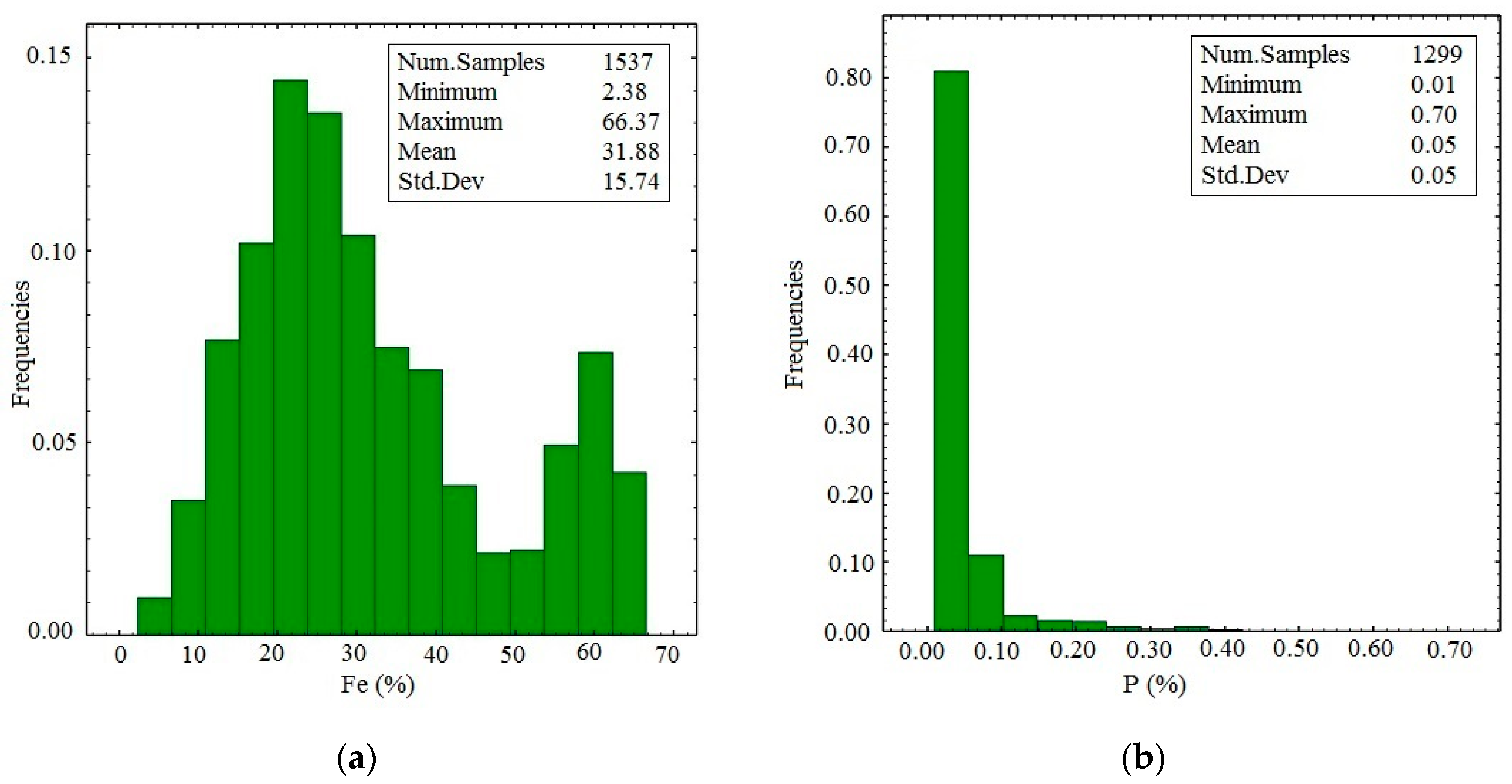
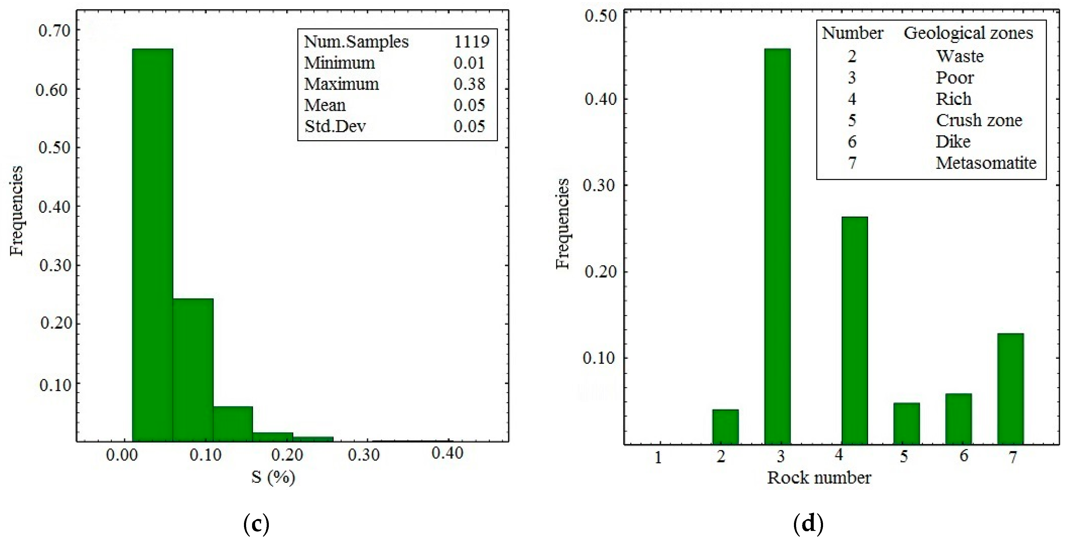
Minerals 09 00115 g002
Figure 3. Histograms of borehole samples obtained from Fe (%) (a), P (%) (b), S (%) (c) and the distribution of borehole samples in each geologic domain (d).
Minerals 09 00115 g003aMinerals 09 00115 g003b
Figure 4. The proportions of the grades data in different geologic domains. (a) shows the overlapping of poor, rich and other geological zones, (b) shows the overlapping for waste, metasomatite and other geological zones.
Minerals 09 00115 g004
Figure 5. Elevation Z = 1585 m of blastholes classified by cutoff grade and threshold (horizontal section).
Minerals 09 00115 g005
Figure 6. Vertical sample variogram (black points) and variogram model (red line) for regularized 2.0 m samples for the global model.
Minerals 09 00115 g006
Figure 7. Example of an estimated geologic vertical section using local models (a), and zoom of one specific area (b).
Minerals 09 00115 g007
Figure 8. Sample and modeled variograms of indicators and Fe (%) (direct and cross variograms): Regularized 2.0 m samples in vertical direction.
Minerals 09 00115 g008
Figure 9. Vertical section of the estimated ore body showing indicator co-kriging (ICK) results.
Minerals 09 00115 g009
Figure 10. Contact plot showing the mean Fe (%) in a rich domain (left), and poor domain (right) (a); contact plot showing the mean Fe (%) in a poor domain (left), and metasomatite domain (right) (b).
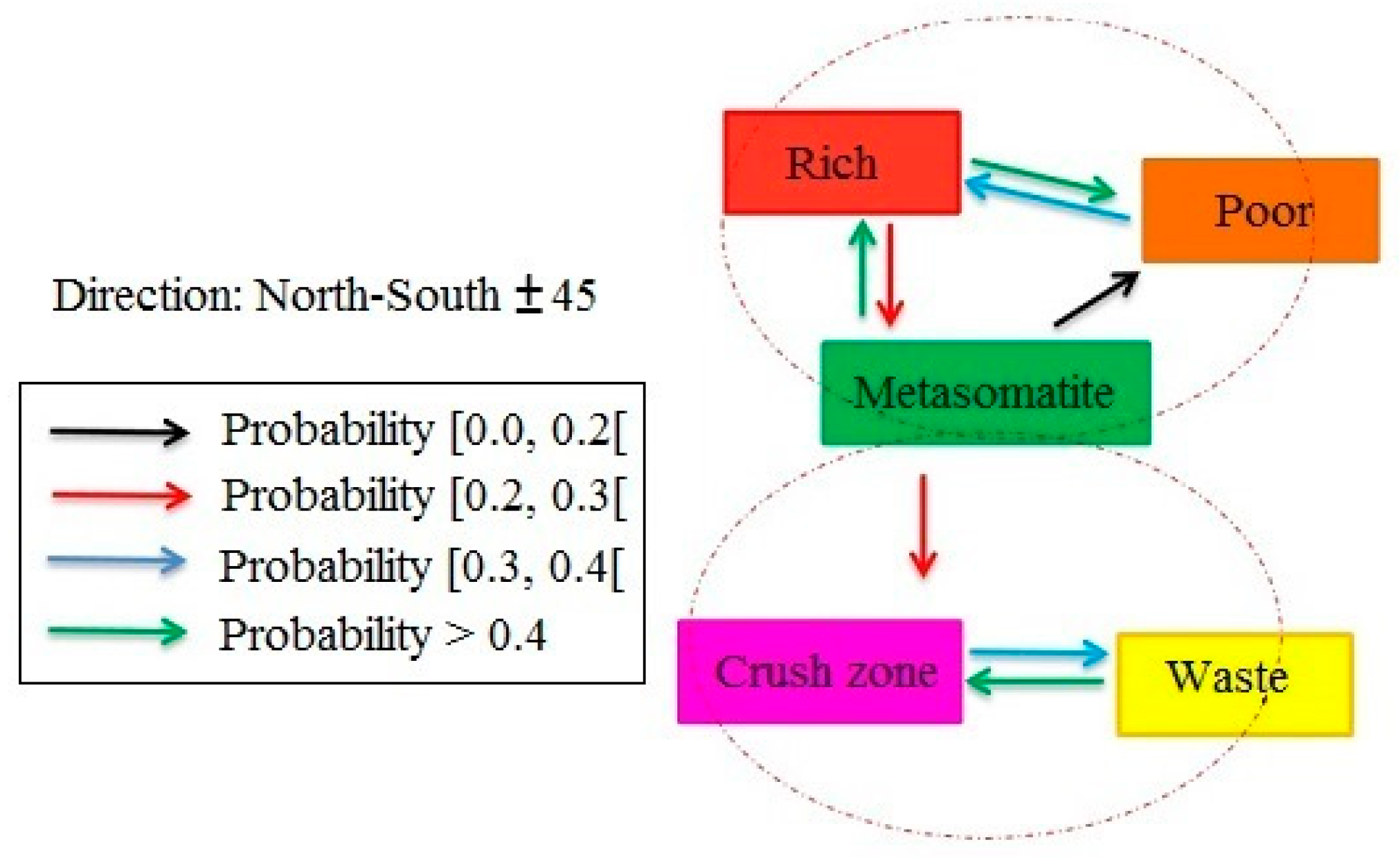
Minerals 09 00115 g010
Figure 11. Preferential relationship schemes in North-South direction (45˚ tolerance). The top section shows domains above cut-off (Fe > 20%), while the lower section indicates domains with Fe < 20%.
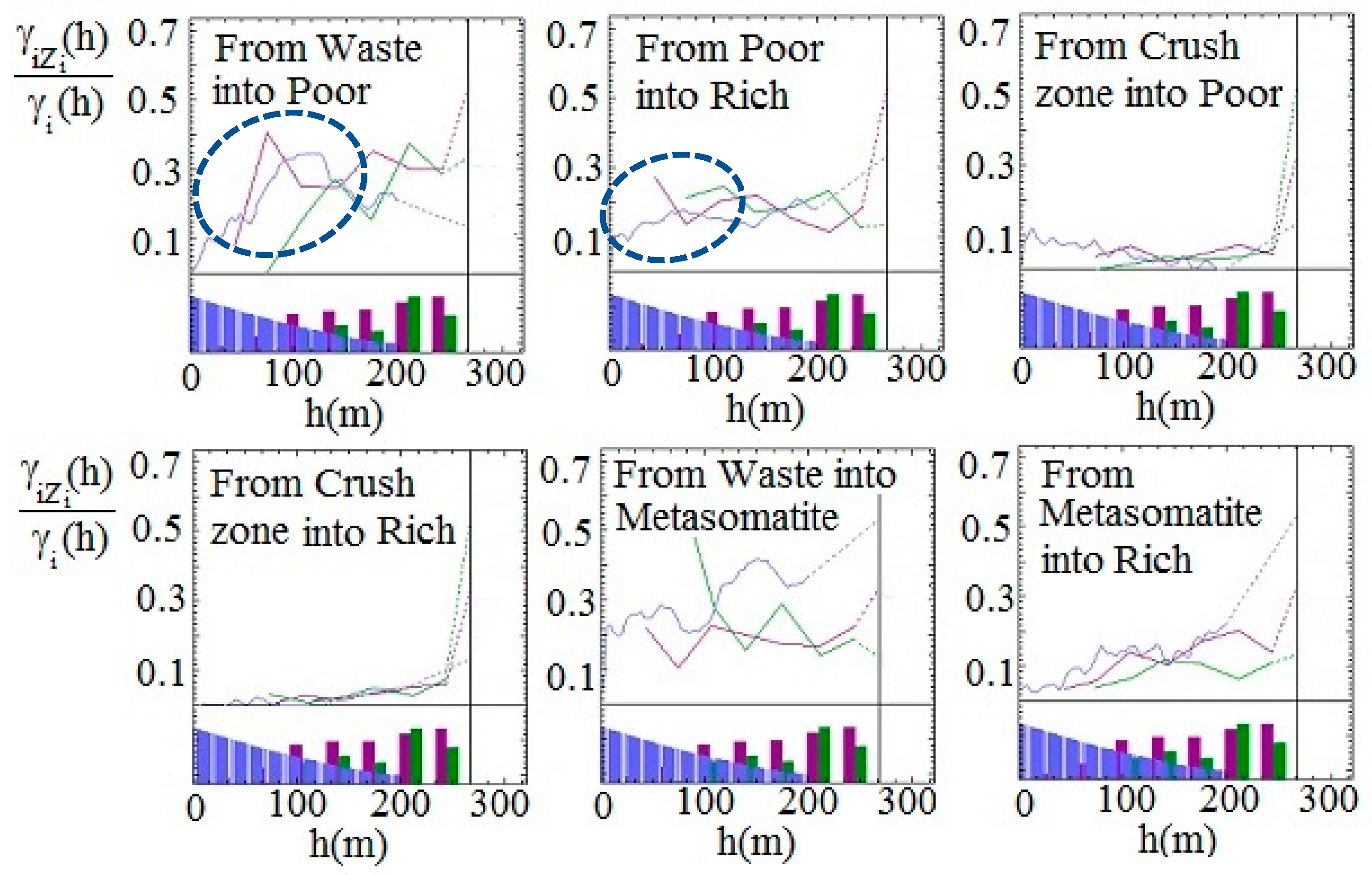
Minerals 09 00115 g011
Figure 12. Variogram ratio between indicator and partial grade divided by indicator variogram in three directions (vertical direction: blue, horizontal directions (0, 90): red and green).
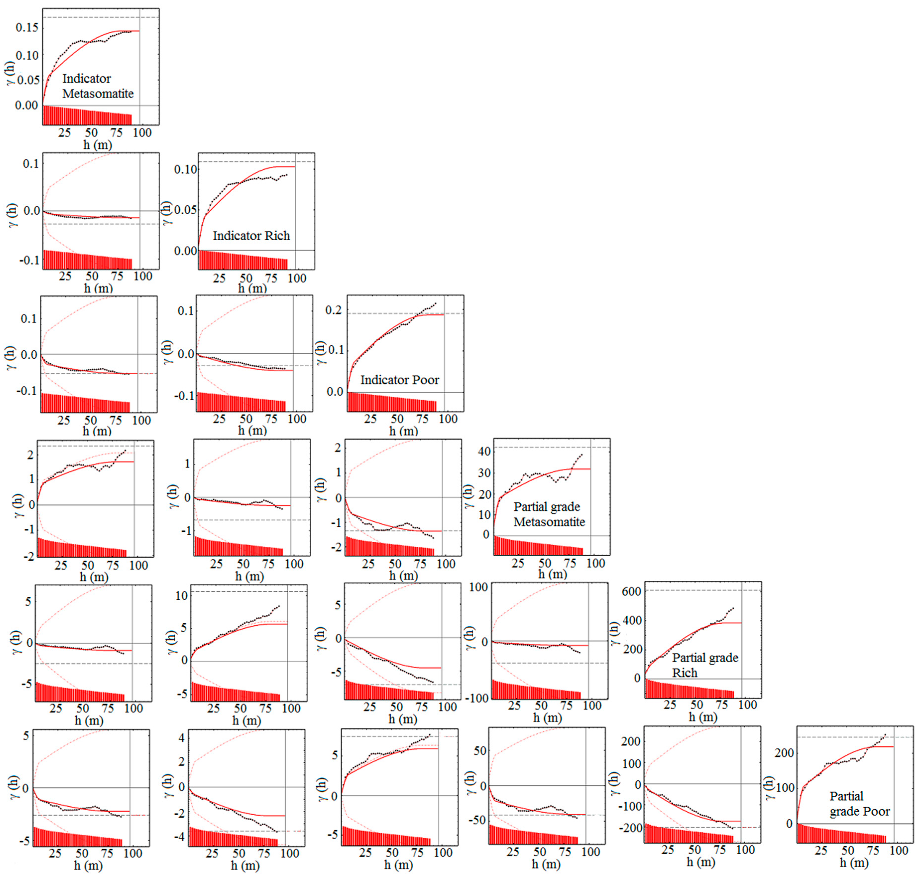
Minerals 09 00115 g012
Figure 13. Sample and modeled variograms of indicators and partial grades (direct and cross variograms): Regularized 2.0 m samples in vertical direction.
Minerals 09 00115 g013
Figure 14. Histogram of true block values obtained from the mean of blastholes (a) and histogram of number of blastholes used for averaging the block values (b).
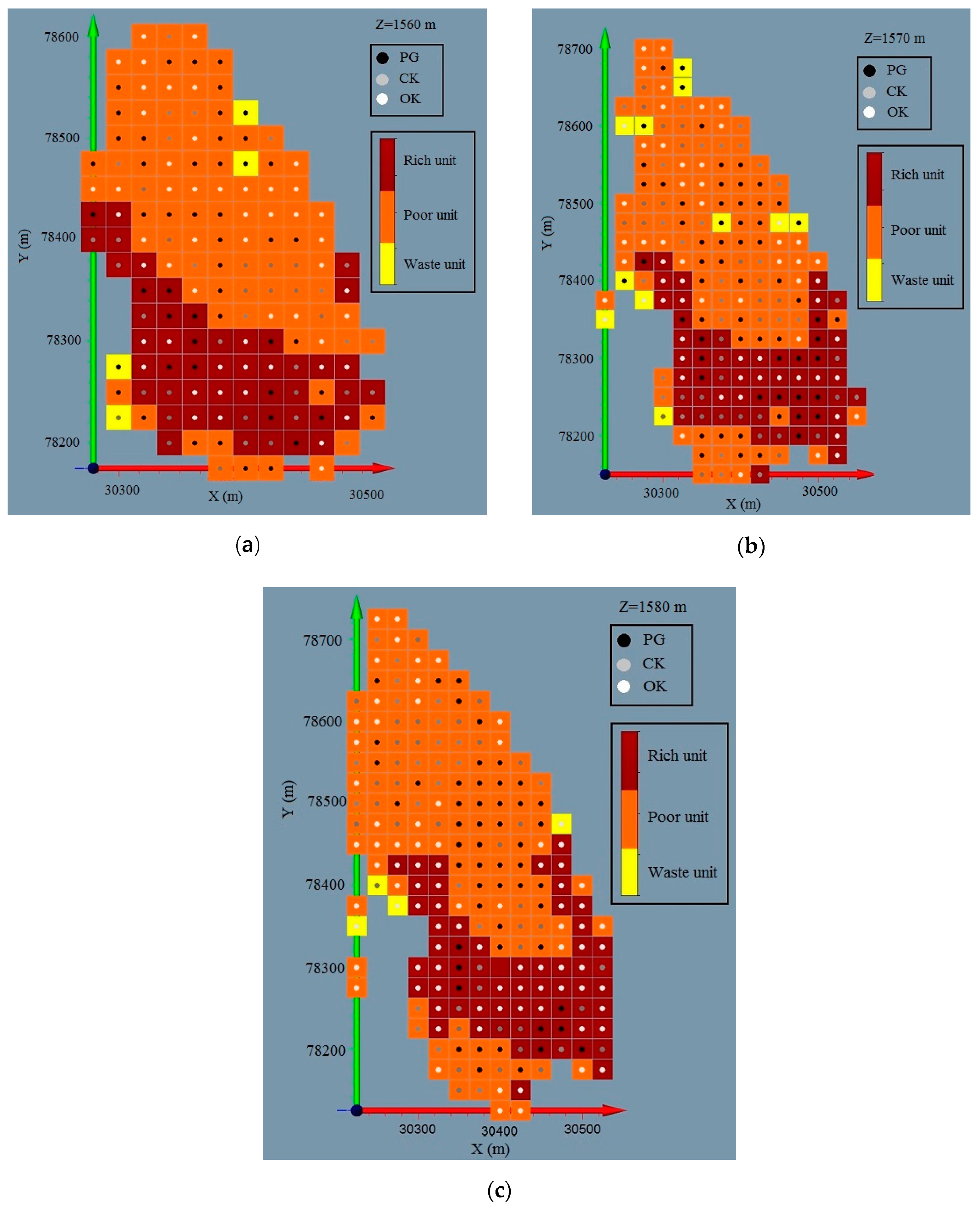
Minerals 09 00115 g014
Figure 15. Maps of real block values obtained from mean of blastholes with optimum estimation method (e.g., three exploited levels). (a) is the horizontal section z = 1560 m, (b) is the horizontal section z = 1570 and (c) is the horizontal section z = 1580 m.
Minerals 09 00115 g015
Table 1. Statistics of the grades.
Variable Number of SamplesMinimumMaximumMean (m)Standard Deviation (σ)Coefficient of Variation (σ/m)
Fe (%)15372.3866.3731.8815.740.49
P (%)12140.010.420.050.061.2
S (%)11140.010.270.050.040.8
Table 2. Statistical parameters of Fe samples in six geologic domains.
Geological Zones of the Iron Deposit Number of DataGrade Fe (%)
MeanMinimumMaximum
Waste4312.542.3826.10
Poor48230.5011.9053.23
Rich27857.2926.1667.79
Crush Zone5115.184.8430.98
Dike6215.623.0546.42
Metasomatite13615.064.1128.37
Table 3. Histogram, sample variogram (black points) and the variogram model (red line) for regularized 2.0 m samples for local models (waste, poor and rich domains).
Exploited DomainsHistogram Variogram
Poor zone Minerals 09 00115 i001 Minerals 09 00115 i002
Rich zone Minerals 09 00115 i003 Minerals 09 00115 i004
Waste zone Minerals 09 00115 i005 Minerals 09 00115 i006
Table 4. Cross-validation comparison using local and global models.
MethodOK-Global ModelOK-Local PoorOK-Local RichOK-Local Waste
Mean error (%)−0.140.471.55−2.25
Variance error (%)226.4541.6435.7224.85
Variance standardized error0.891.030.701.37
Table 5. Cross-validation comparison using global models and local model with adjacent domain data.
MethodOK-Global ModelOK-Local PoorOK-Local RichOK-Local Waste
Mean error (%)−0.140.14−0.15−0.13
Variance error (%)226.4527.8827.2027.68
Variance standardized error0.890.800.820.63
Table 6. Cross-validation using the co-kriging (CK), partial grade (PG) and ordinary kriging (OK)-global models.
MethodsMean-Error (%)Variance-Error (%)2Variance of Standardized Error (%)2
Partial Grade−0.1227.730.83
CK-with indicators at target points−0.0217.900.82
CK- without indicators at target points0.1226.080.99
OK global model−0.0928.221.04
Table 7. Quantification of the optimal use of the estimation method in the case study.
Levels (m)Total Number of BlocksNumber of Blocks for Zone and Geological Methods
Rich Zone Poor ZoneWaste Zone
OKCKPGOKCKPGOKCKPG
Z = 154031502587103
Z = 155010018147171720403
Z = 1560145191813342235013
Z = 1570183241717353841416
Z = 158020346810405045310
Z = 159020352124394352100
Z = 16002035892414048131
Z = 16101896460504022241
Total12572868455261258270161017
Total (%)125722.7%6.68%4.4%20.8%20.5%21.5%1.3%0.8%1.3%

