1. Introduction
A geological model consists of a three-dimensional representation of an ore deposit constructed by resource geologists on the basis of their knowledge of the deposit, geological field observations, geophysical surveys, and drill hole logs and assays. A geological model that represents the spatial locations and extents of rock types or ore types is an essential input for mineral resources evaluation and mine planning and, as such, affects all subsequent stages of the mining process [
1,
2,
3,
4,
5]. The typical workflow for assessing mineral resources consists of grouping the rock types or ore types into geological domains in which the quantitative variables of interest (geochemical, geometallurgical, and/or geomechanical variables) are assumed to be homogeneously distributed and then interpolating these variables within each domain using geostatistical techniques. This hierarchical workflow accounts for geological controls on the distributions of the quantitative variables but produces clear-cut discontinuities in the values of the quantitative variables when crossing the domain boundaries [
5,
6]. Several alternatives have been proposed to mitigate these discontinuities and to account for spatial correlation across the domain boundaries [
6,
7,
8,
9,
10]. Another approach to produce gradual transitions near the domain boundaries is to model the quantitative variables of interest with no previous geological domaining by considering the controlling rock types or ore types as cross-correlated covariates [
11,
12,
13,
14,
15,
16].
Geostatistical simulation approaches have been designed to construct several geological scenarios in order to quantify uncertainty in the actual locations and extents of rock types or ore types, accounting for their spatial continuity and proportions (which may vary in space), and contact relationships, including chronological associations, allowable and non-allowable contacts, edge effects (preferential contacts), and directional effects (asymmetrical spatial relationships) between rock types or ore types ([
17,
18,
19,
20] and references therein). However, these approaches are still in their infancy in practical orebody modelling where the geological model often corresponds to a single interpretation of the deposit, rather than multiple scenarios, which does not allow geological uncertainty to be measured. This motivates the need for quantitative methods to validate the model and to identify the areas of the deposit that have higher probabilities of being misinterpreted.
Most published research on geological modelling focuses on using all available data to generate a more accurate geological model, e.g., by using structural and geophysical data together in addition to drill hole data or by using data inversion methods to generate an interpreted model [
21,
22]. Studies of validating geological models often concentrate on statistical and graphical analyses by comparing the models with the available data to detect inconsistencies [
5].
In this work we propose a geostatistical approach to construct simulated geological scenarios and to validate an interpreted geological model by identifying the areas of a deposit that are likely to be misinterpreted. The approach relies on the analysis of quantitative variables that are measured at sampling locations and are cross-correlated with the geological categories obtained from geological core logging. It includes the geostatistical modelling and simulation of the quantitative variables, followed by their classification into geological categories. Comparing the prior (without sampling information) and posterior (accounting for sampling information) probabilities of categories for each target location provides a means of identifying the locations that are most likely to be incorrectly interpreted.
The paper is outlined as follows:
Section 2 comprises the case study and the methodology used to model, simulate, and classify the quantitative variables of interest.
Section 3 presents the results of comparing the prior and posterior probabilities of geological categories to identify potentially misinterpreted blocks. Conclusions and perspectives follow in
Section 4.
2. Materials and Methods
2.1. Case Study Presentation
The case study is a banded-iron formation (BIF)-hosted iron ore deposit for which there are 4177 diamond drill core samples. For reasons of confidentiality, the name and location of the deposit are not disclosed and a local coordinate system is used. Seven quantitative variables have been analysed for each sample: the grades of iron (Fe), silica (SiO
2), phosphorus (P), alumina (Al
2O
3), manganese (Mn), loss on ignition (LOI), and the granulometric fraction of fragments with size above 6.3 mm (G). In addition, for each sample, the dominant rock type is available from geological logging, which is coded into ten categories: friable hematite (code 1), compact hematite (code 2), alumina-rich hematite (code 3), alumina-rich itabirite (code 4), manganese-rich itabirite (code 5), compact itabirite (code 6), friable iron-poor itabirite (code 7), friable iron-rich itabirite (code 8), amphibolitic itabirite (code 9), and canga (code 10). There are dependent relationships between the quantitative variables and the rock codes [
23], as summarised in
Table 1. This implies that information about the former may help to detect inconsistencies in the interpretation of the latter, which is the basis of the proposed geostatistical methodology.
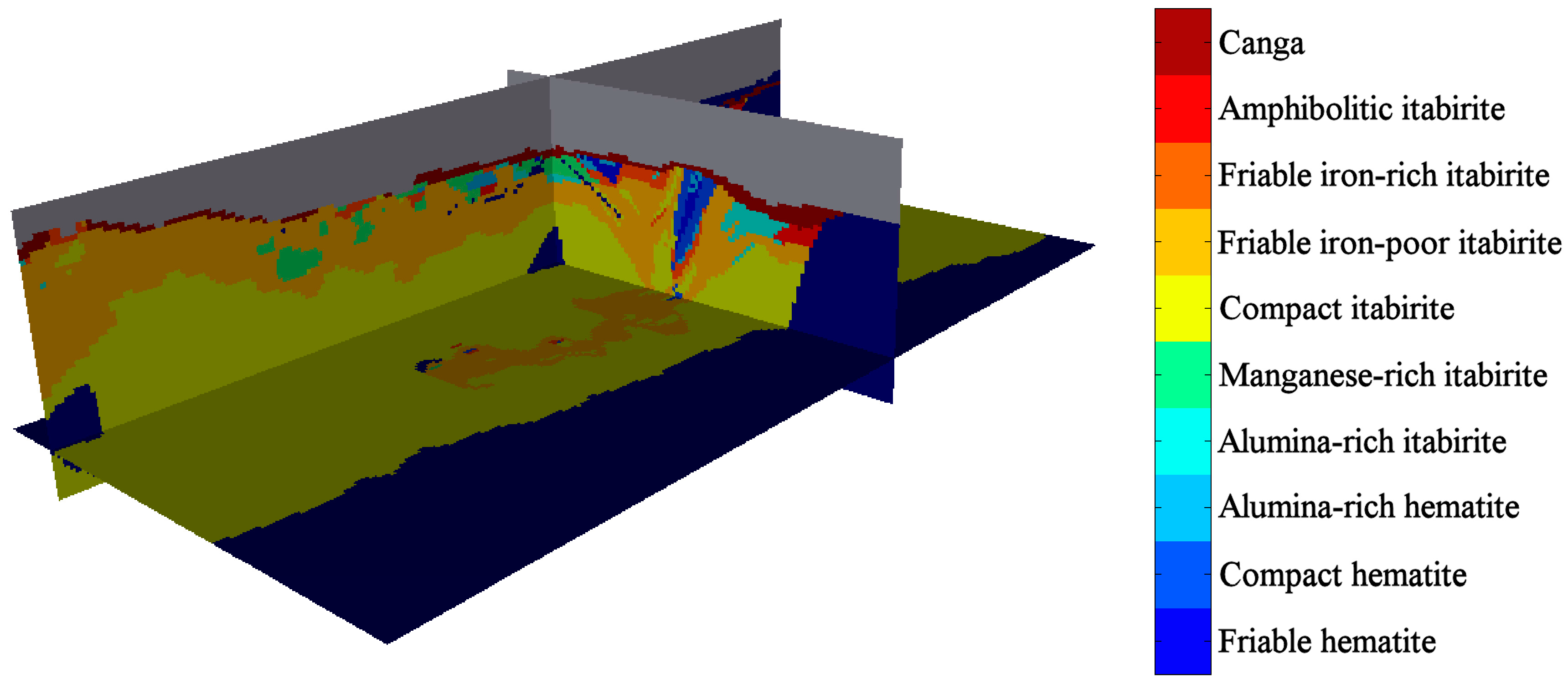
Based on the drill hole information and their knowledge of the deposit, the resource geologists constructed two-dimensional representations of the rock type distribution in specific plan views and cross-sections, then interpolated these representations with indicator kriging to construct a rock type model (the most probable rock type, obtained by post-processing the indicator kriging results) on a 3D grid with a regular spacing of 10 m × 10 m × 10 m (
Figure 1). This 3D model is the basis for mineral resource evaluation and for mine planning, but does not provide any quantification of the uncertainty in the actual rock type assigned to each block. It is therefore of interest to design a method for validating the interpreted rock type assigned to each grid block and for finding the blocks for which the interpretation is likely to be mistaken.
In the following, we will exclude the waste rocks in the outer parts of the deposit, as well as the canga in the superficial part, as their locations and extents depend more on geographical position than on the quantitative variables. Accordingly, the following stages of the study will be restricted to the underlying ferruginous rock (rock types 1–9).
2.2. Modelling and Simulation of Quantitative Variables
Adeli and Emery [
24] presented a hierarchical model for this deposit, in which the rock type controls the distribution of the quantitative variables (Fe, SiO
2, P, Al
2O
3, Mn, LOI, G) and the spatial correlation structure of these variables depends on the prevailing rock type domain. In the following, we will reverse this point of view and assume that the rock type is subordinate to the quantitative variables. In other words, the quantitative variables will be modelled and simulated throughout the deposit without any previous geological domaining. Because of the relationship between the grades, granulometry, and rock types (
Table 1), the rock type will then be allocated on the basis of the simulated values of these quantitative variables by means of a classification algorithm. Unlike the aforementioned hierarchical model, this approach does not produce discontinuities in the values of the quantitative variables near the rock type boundaries, which conforms with the concept of a disseminated ore deposit [
14,
15]. In this deposit, the quantitative variables are spatially correlated across the rock type boundaries, as shown in [
10,
24].
2.2.1. Change of Variables Based on Stoichiometric Closure
A joint simulation approach is required to reproduce the dependence relationships among the quantitative variables. In particular, the grade variables are linked through the following stoichiometric closure formula:
in which the coefficients 1.4297, 2.2913, and 1.2912 are used to rescale the masses of iron (Fe), phosphorus (P), and manganese (Mn) to the masses of hematite (Fe
2O
3), phosphorus pentoxide (P
2O
5), and manganese monoxide (MnO), respectively. A convenient way of reproducing the stoichiometric closure in the simulated grade values is to conduct a change of variables. Some alternatives for such a change of variables are the additive logratio (alr), centred logratio (clr), or isometric logratio (ilr) transformations that are often used in compositional data analysis [
25], but these transformations are not suitable for variables that can take zero values, as is the case in the present case study. We therefore opt for a ratio transformation that does not use logarithms, as proposed in [
10], where the quantitative variables are successively normalised by the residual of the closure:
In the above equation, the original variables have been ordered from the variable with the lowest mean value (P) to the variable with the highest mean value (SiO
2) in order to minimise the distortion induced by the ratio transformation (the correlation coefficients between Z
1 and P, Z
2 and Mn, Z
3 and Al
2O
3, Z
4 and LOI, and Z
5 and SiO
2 are all greater than 0.995 [
10]). The transformed variables have no stoichiometric constraint and take their values in the interval [0–1). Note that there are only five unconstrained transformed variables (Z
1–Z
5) instead of six constrained grade variables (Fe, SiO
2, P, Al
2O
3, Mn, LOI). The back-transformation is obtained from Equations (1) and (2):
2.2.2. Projection Pursuit Multivariate Transformation
The data for the five unconstrained variables (Z
1–Z
5) and granulometry (G) are transformed into multivariate Gaussian data, hereafter called “normal scores”. Because of the heteroscedastic dependence relationships between the variables prior to transformation (
Figure 2), the normal scores transformation of each variable separately [
26] does not provide truly multivariate Gaussian data. For instance, the scatter diagram between any two transformed variables does not have an elliptical shape, which indicates that these transformed variables do not correspond to jointly Gaussian random fields. To avoid this inconvenience, a joint normal scores transformation can be used, such as stepwise conditional transformation (SCT) [
27], flow transformation (FT) [
28], or projection pursuit multivariate transformation (PPMT) [
29,
30,
31]. All these methods require all the variables to be known at all the data locations (isotopic sampling), which is the case in the present case study; otherwise, the data set should be completed by multivariate imputation techniques [
32] before joint normal scores transformation. In practice, the first two approaches are still limited to few variables (SCT) or to small data sets (FT), and for this reason we chose the third approach (PPMT) here. The PPMT transformation is based on an iterative algorithm and allows the complex dependence relationships (such as nonlinearities and heteroscedasticities) between cross-correlated variables to be removed, providing a set of new variables that are normally distributed and uncorrelated at collocated locations [
29,
30,
31]. The transformation uses declustering weights to account for the uneven positions of the drill hole data in space. For each rock type, the weights are obtained by considering the ratio of the rock type proportion in the interpreted geological model and the rock type proportion in the drill hole data. It is assumed here that the interpreted model, which is constructed from the drill hole information and geological knowledge of the deposit, is globally accurate, i.e., it provides a reliable estimate of the true rock type proportions, although it may be locally inaccurate as some blocks may be misinterpreted.
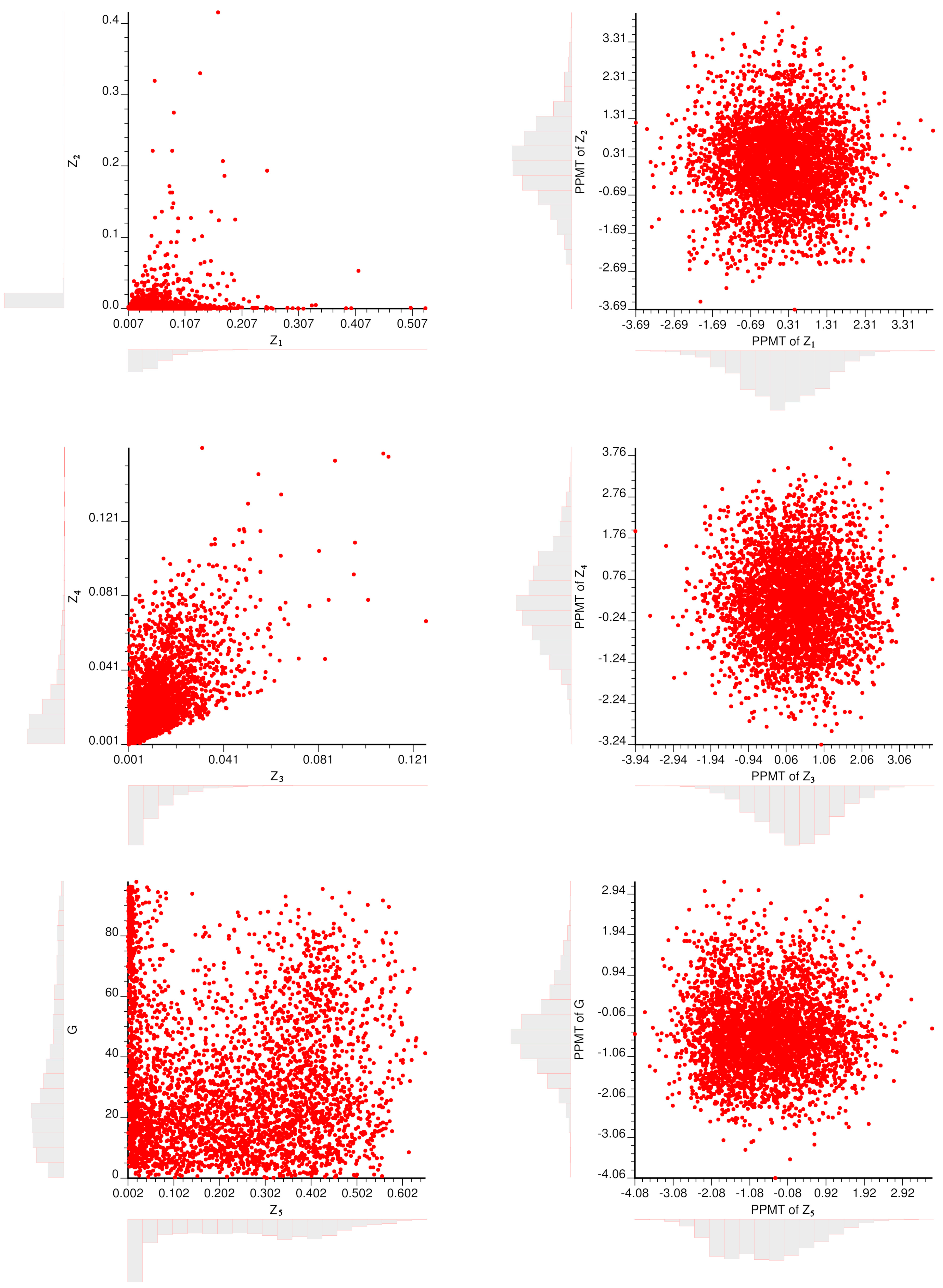
Figure 2 shows how PPMT transforms the joint distribution of the quantitative variables (Z
1, Z
2, Z
3, Z
4, Z
5, G) into a multi-Gaussian one. The marginal distributions (histograms) are bell-shaped, while the bivariate distributions (scatter plots) exhibit the typical circular shape of uncorrelated Gaussian variables.
2.2.3. Spatial Continuity Modelling
The PPMT transformed variables are represented by jointly stationary Gaussian random fields within the studied area. By construction, these random fields have a mean of zero, so that their finite-dimensional distributions are fully characterised by their direct and cross-covariance functions. Under an additional assumption that the cross-covariances are even functions, one can use the direct and cross-variograms as an alternative to the covariances; this additional assumption implies the absence of asymmetries, such as spatial shifts or delay effects, in the spatial cross-correlation between variables [
33].
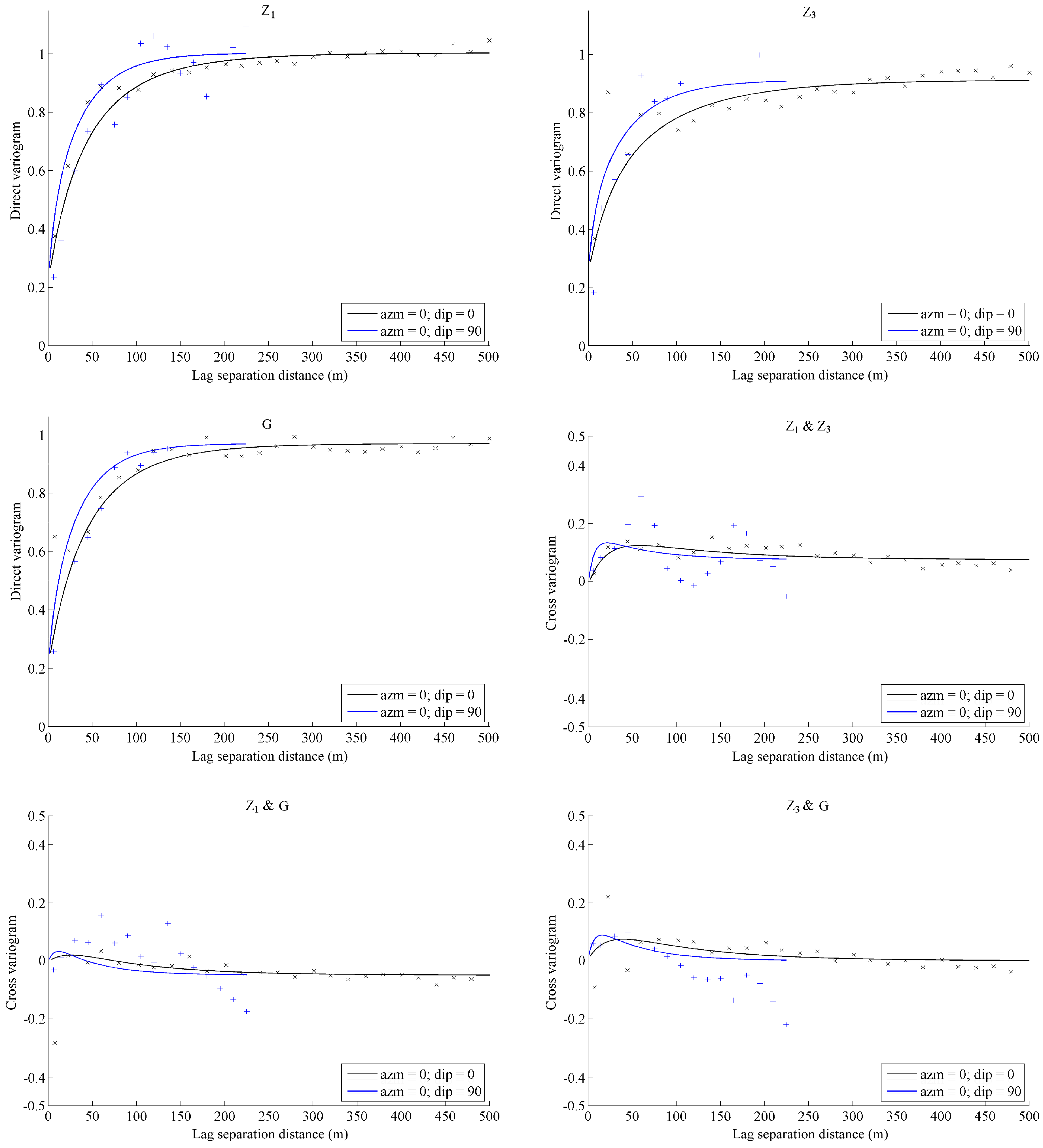
In the first step, the spatial correlation structure of the normal scores data is inferred by calculating their experimental direct and cross-variograms (six direct variograms and fifteen cross-variograms) along the horizontal and vertical directions, which were identified as the main anisotropy directions. The cross-variograms indicate a low correlation (not necessarily zero) between two different random fields taken at different locations (separation distances greater than zero). The direct variograms tend to a sill value close to one, which corroborates the validity of the stationarity assumption, at least at a local scale (quasi-stationarity) [
26]. Based on this observation, a linear model of coregionalisation [
32] consisting of nested exponential models is fitted to the direct and cross-variograms, by using a semi-automated algorithm to find the sill matrices associated with the nested structures that minimise the squared differences between experimental and theoretical variograms [
34,
35] (
Figure 3). A simplified model, in which the cross-variograms are exactly zero and the PPMT-transformed variables are spatially independent, could also be considered, which amounts to neglecting the cross-correlation between these variables. The full model (with non-zero cross-variograms) is used in the following, as it is not significantly more complex.
2.2.4. Conditional Simulation
The Gaussian random fields are jointly simulated using a spectral turning-bands algorithm [
36]. This algorithm is preferred to other alternatives, such as sequential, covariance matrix decomposition or circulant-embedding algorithms ([
26] and references therein) because of its accuracy, versatility, unequalled computational speeds, and low memory storage requirements, being able to simulate highly-multivariate random fields and to reproduce exactly the desired spatial correlation structure [
36].
Twenty realisations are constructed on the same grid as the interpreted rock type model. These realisations are then conditioned to the PPMT-transformed data known at the drill hole locations by using post-conditioning cokriging [
26] and finally back-transformed into grades and granulometry. To account for possible deviations from strict stationarity, the conditioning to data is performed by ordinary cokriging, which allows the mean values of the Gaussian random fields to vary locally (i.e., at the scale of the cokriging neighbourhood) and to reproduce the spatial trends exhibited by the conditioning data (an exception would be for extrapolation situations, but grid nodes located far away from the data are not the target of the proposed methodology) [
13,
37,
38]. As an illustration, two realisations are shown in
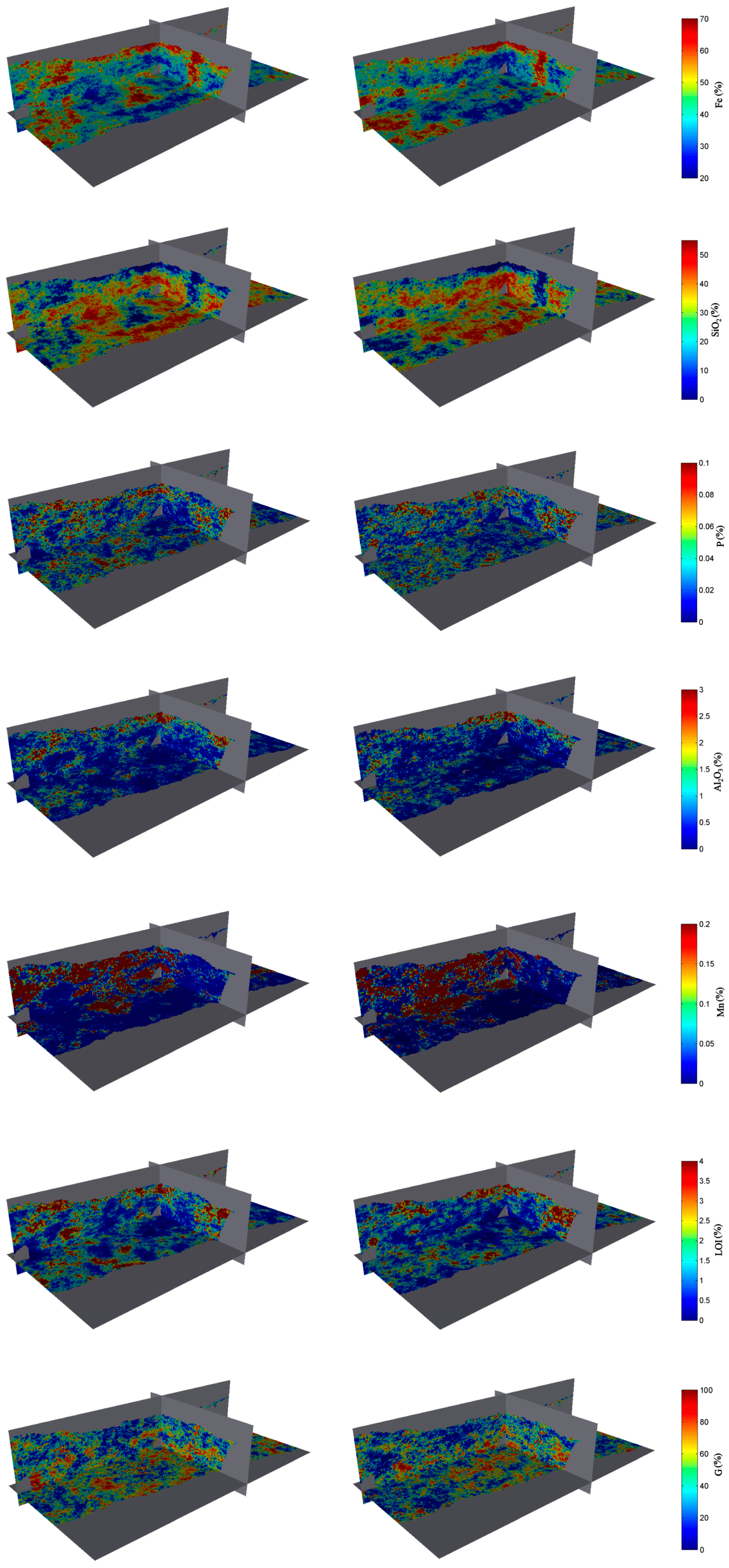
Figure 4. More than 20 realisations could have been constructed, but this would increase not only the computational time to run the simulation (a few hours on a common desktop) and the memory requirements to store the simulated values, but also the combination of the results to be treated (support of the multinomial distribution used to model the combinations of rock type occurrences among the realisations, see Equation (4) in
Section 2.5).
2.2.5. Checking the Realisations
The correlation coefficients of drill hole data and simulated grades and granulometry are shown in
Table 2, while
Figure 5 displays the scatter diagrams of three pairs of variables. Both tools show that the simulated values accurately reproduce the bivariate distributions of the data values [
39]. Furthermore, by construction, the realisations also reproduce the stoichiometric closure (imposed by the change of variables), the spatial continuity (imposed by the direct and cross-variograms), and the conditioning data (imposed by post-conditioning cokriging).
2.3. Construction of Simulated Geological Scenarios by Classification
A classification algorithm is now used to assign a rock type from 1 to 9 for each realisation and each target grid block depending on the values of the simulated quantitative variables. To choose the algorithm, several classifiers are trained on the drill hole data set and compared through a stratified 10-fold cross-validation. Specifically, the drill hole data set (containing information on both the rock type and the quantitative variables) is divided randomly into ten subsets; each subset is held out, the classifier is trained on the remaining nine subsets and tested on the holdout subset, and its error rate is calculated. This procedure is executed in its entirety 10 times on different training subsets; ultimately, the ten error rates are averaged to get an overall error estimate [
40]. A geographical selection could be used instead of a random selection to define the ten data subsets, so as to reduce the redundancies between the training and testing subsets. However, the direct variograms of the normal scores data (
Figure 3) exhibit a significant nugget effect (more than 25% of the total sill), so that the redundancies are low, even when using a random selection. Note that this training stage is the only instance in our proposed approach that uses the rock type data logged on the drill hole samples.
The classifier that obtained the best results was the Simple Cart algorithm, with an error rate less than 18% (
Table 3). This classifier is a decision tree algorithm; it is a logical choice given the associations between rock types and quantitative variables indicated in
Table 1. Note that an error rate of 0% is not desirable since the logged rock type is a qualitative property obtained from geological core logging and is not error-free (unlike the quantitative measurements, which are assumed to be accurate) [
24]. In addition, the incorrectly classified rock type data can be identified as the most likely to be mis-logged and be the priority candidate for checking (relogged) to ensure data consistency.
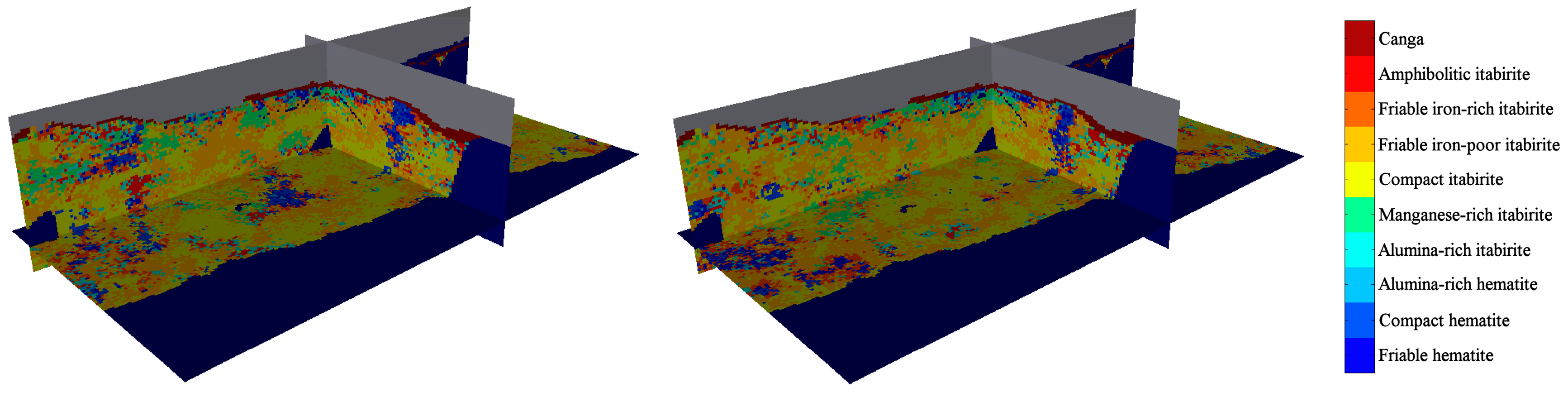
The classification applied to the 20 conditional realisations resulted in a number of occurrences of each rock type (from 0 to 20) for each target grid block.
Figure 6 shows the classified rock type for two realisations.
2.4. Determining the Prior Probability of Occurrence of Each Rock Type
It is of interest to determine whether the conditioning drill hole information influences the classification results for each target block. To do so requires the prior probabilities of all rock types to be determined by classifying the grades and the granulometry simulated in the absence of the conditioning drill hole data. In detail, the simulation process is then repeated, this time without any conditioning data, to produce 1000 realisations of the grades and granulometry. These non-conditional realisations provide the prior probabilities (
p1, …,
p9) of the different rock types by counting the numbers of occurrences of each rock type across the 1000 realisations (
Table 4). This only requires one block to be simulated because the prior probabilities are the same for all the blocks in the deposit.
2.5. Comparing the Prior and Posterior Probabilities of Rock Type Occurrences to Identify Potentially Misinterpreted Blocks
Knowing the prior probability of occurrence of each rock type, the prior distribution of the rock types that should be observed on a limited set of independent realisations can be modelled as a multinomial distribution [
41]:
In particular, this distribution gives the probability of any particular combination of the numbers of occurrences for the nine rock types among twenty (n = 20) realisations in the absence of effects of conditioning drill hole data.
If, for a given block, the numbers of rock type occurrences that are observed among the twenty conditional realisations constitute an unlikely combination of the prior multinomial distribution, then it can be concluded that the drill hole data has a significant effect on that block, i.e., there is statistical evidence that the drill hole data convey information about the rock type for this particular block. If, in addition, the rock type interpreted by the resource geologists has a low frequency of occurrence (posterior probability) among the twenty conditional realisations, then the block can be identified as potentially misinterpreted.
The statements in the previous paragraph require a quantitative definition of “unlikely” or “low”. To this end, the combinations of the prior multinomial distribution are ranked, from the least probable to the most probable, and the less probable combinations (up to a cumulative probability of 0.1) are classified as “unlikely” or “improbable”. One then looks for the blocks in which such improbable combinations arose in the twenty conditional realisations, i.e., the combination is very unlikely in the non-conditional case (absence of drill hole data) but has occurred in the conditional case, showing that there is a significant effect of the conditioning drill hole data on the blocks. Note that there is no particular reason to find 10% of the blocks in the geological model with the above-specified cumulative probability (0.1): more blocks may exhibit an “unlikely” combination if the conditioning data have a strong effect (long-range correlation structure), while fewer blocks (possibly none) may be identified if the conditioning data have low spatial correlation.
Finally, the following three criteria are used to identify potentially misinterpreted blocks among the blocks that are significantly affected by the drill hole data: (i) the prior probability of the rock type interpreted by the geologists is greater than its posterior probability; (ii) the posterior probability of the rock type interpreted by the geologists is less than 0.15 (unlikely); and (iii) another rock type has a posterior probability higher than the posterior probability of the rock type interpreted by the geologists and has been logged at a drill hole sample less than 60 m away from the block. This last criterion is adopted to avoid extrapolating the drill hole information too much, bearing in mind that the geostatistical model is likely to be valid only at a local scale (quasi-stationarity assumption) and considering a distance lower than the spatial correlation range, for which the direct variograms reach about 70–80% of their sills (
Figure 3). The particular values (0.15 probability and 60 m distance) chosen in criteria (ii) and (iii) can nevertheless be tuned by the user depending on his/her preferences, intuition, and expertise (or be modified in other case studies, depending on the observed correlation range of the quantitative data), which reflects more or less conservative detections of the misinterpreted rock types in the geological model.
3. Results and Discussion
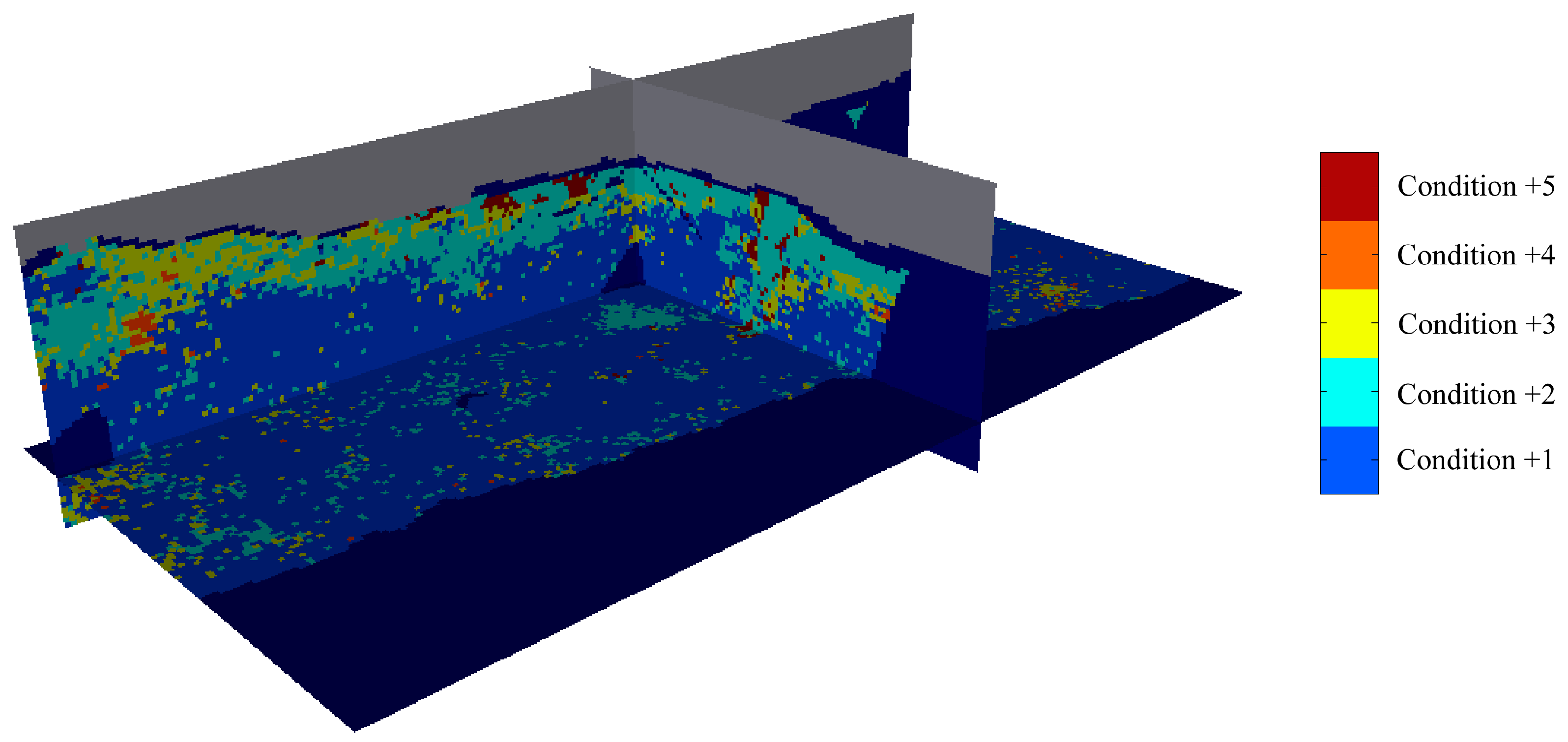
The application of the criteria in the previous section identifies 3.39% of all the blocks (20,999 blocks out of 619,919 blocks flagged with rock types 1–9 in the original geological model) to be potentially misinterpreted (condition +5), as shown in
Figure 7. Conditions +1 to +5 are described in
Table 5.
Except for a few blocks scattered across the deposit, the identified misinterpreted blocks (condition +5) are concentrated in the upper part of the ore deposit, in the margins of the manganese-rich itabirite, alumina-rich itabirite, and hematite bodies, showing the necessity to check these blocks in order more accurately to separate these bodies located in the transitional parts of the deposit from high to low manganese, alumina, and iron grades.
The numbers of correctly interpreted and potentially misinterpreted blocks for each interpreted and suggested rock type are shown in
Table 6. For example, 35 blocks are interpreted as rock type 1 (friable hematite) with the suggestion they be changed to rock type 2 (compact hematite).
In the following, three of the potentially misinterpreted blocks are selected and discussed in light of the simulated values of grades and granulometry. For the first selected block (referred to as “block n°1”), with easting coordinate 340 m, northing coordinate 380 m, and elevation −40 m in the local coordinate system, the mining geologist interpretation corresponds to rock type 6 (compact itabirite). However, the simulated values of granulometry (mostly less than 50%) suggest that this block should actually be interpreted as rock type 7 (friable iron-poor itabirite) in 17 out of the 20 realisations (
Table 7). This rock type code (7) is also the one logged in the three closest drill hole samples, all of which are less than 20 m from block 1. A similar situation occurs for block n°2 with easting coordinate −580 m, northing coordinate 330 m, and elevation 280 m, interpreted as rock type 7 (friable iron-poor itabirite), which is re-interpreted as rock type 1 (friable hematite) in 17 out of the 20 realisations, based on the high simulated iron grades (
Table 8); the four nearest drill hole samples, less than 35 m from the block, have been logged as rock type 1, which corroborates the suggestion for a re-interpretation of the block. For block n°3 with easting coordinate 1390 m, northing coordinate 410 m, and elevation 390 m, 17 of the 20 realisations suggest classification as rock type 3 (alumina-rich hematite), based on the high simulated iron and alumina grades (
Table 9), whereas the original geological interpretation corresponds to rock type 8 (friable iron-rich itabirite). This interpretation (rock type 8) coincides with the log of the closest sample, less than 30 m from the block, but examination of the grades of this sample suggests that it may actually be mis-logged: following the methodology proposed in [
24], the
p-values of rock types 3 and 8 are 0.94 and 0.51, respectively, indicating that the former code is more plausible than the latter.
On a final note, the proposed methodology used for validating the interpreted geological model, based on the calculation of prior and posterior probabilities, and on the definition of heuristic criteria (
Section 2.4 and
Section 2.5), can be applied not only to the geological scenarios obtained from the simulation and classification of quantitative covariates, as set out in
Section 2.2 and
Section 2.3, but also to scenarios obtained from any other geostatistical simulation method, e.g., multiple-point, truncated Gaussian or plurigaussian simulation [
17,
18,
19,
20].
4. Conclusions
The rock type or ore type model interpreted by mining geologists is the basis for mineral resource evaluation, mine planning, and subsequent stages of the mining process. This motivates the design of a method for validating the interpreted category assigned to each grid block and for finding the blocks for which the interpretation is likely to be incorrect. To this end, a geostatistical-based approach has been proposed for constructing a set of simulated geological scenarios and for identifying potentially misinterpreted blocks, assuming that there is a clear association between geological categories and measured quantitative covariates.
The applicability of the proposal was tested on an iron ore deposit in which there is a clear association between the interpreted rock types and seven quantitative covariates (grades of iron, silica, phosphorus, alumina, manganese, loss on ignition, and granulometry). The proposal combines a change of variables based on a stoichiometric closure formula, PPMT transformation, variogram analysis, turning-bands simulation, post-conditioning cokriging, and decision-tree classification. The potentially misinterpreted blocks are then identified by comparing the prior and posterior rock type probabilities, and by defining heuristic criteria that can be tuned by the user to achieve more or less conservative detections.
The proposed approach can be applied not only in the context of geological modelling, but also in the wider context of geometallurgical modelling, in which there are relatively large volumes of multivariate data of different natures and qualities (e.g., grades, grain sizes, mineralogy, alteration, grindability indices, and metal recoveries), and where the correct identification and interpretation of geometallurgical domains is critical to improving process performance.
Acknowledgments
The first two authors acknowledge funding from the Chilean Commission for Scientific and Technological Research through Project CONICYT/FONDECYT/REGULAR/N°1170101. The authors are grateful to two anonymous reviewers for their constructive comments on a previous version of this work.
Author Contributions
Amir Adeli, Xavier Emery, and Peter Dowd conceived and designed the experiments. Amir Adeli performed the experiments. Amir Adeli and Xavier Emery wrote the paper.
Conflicts of Interest
The authors declare no conflict of interest. The founding sponsors had no role in the design of the study; in the collection, analyses, or interpretation of data; in the writing of the manuscript; and in the decision to publish the results.
References
- Duke, J.H.; Hanna, P.J. Geological interpretation for resource modelling and estimation. In Mineral Resource and Ore Reserve Estimation—The AusIMM Guide to Good Practice; Edwards, A.C., Ed.; Australasian Institute of Mining and Metallurgy: Melbourne, Australia, 2001; pp. 147–156. [Google Scholar]
- Sinclair, A.J.; Blackwell, G.H. Applied Mineral Inventory Estimation; Cambridge University Press: New York, NY, USA, 2002; p. 381. [Google Scholar]
- Knödel, K.; Lange, G.; Voigt, H.J. Environmental Geology: Handbook of Field Methods and Case Studies; Springer: Berlin/Heidelberg, Germany, 2007; p. 1357. [Google Scholar]
- Marjoribanks, R. Geological Methods in Mineral Exploration and Mining; Springer: Berlin/Heidelberg, Germany, 2010; p. 238. [Google Scholar]
- Rossi, M.E.; Deutsch, C.V. Mineral Resource Estimation; Springer: London, UK, 2014; p. 332. [Google Scholar]
- Ortiz, J.M.; Emery, X. Geostatistical estimation of mineral resources with soft geological boundaries: A comparative study. J. S. Afr. Inst. Min. Metall. 2006, 106, 577–584. [Google Scholar]
- Larrondo, P.; Leuangthong, O.; Deutsch, C.V. Grade estimation in multiple rock types using a linear model of coregionalization for soft boundaries. In Proceedings of the 1st International Conference on Mining Innovation; Magri, E., Ortiz, J., Knights, P., Henríquez, F., Vera, M., Barahona, C., Eds.; Gecamin Ltd.: Santiago, Chile, 2004; pp. 187–196. [Google Scholar]
- Vargas-Guzmán, J.A. Transitive geostatistics for stepwise modeling across boundaries between rock regions. Math. Geosci. 2008, 40, 861–873. [Google Scholar] [CrossRef]
- Séguret, S.A. Analysis and estimation of multi-unit deposits: Application to a porphyry copper deposit. Math. Geosci. 2013, 45, 927–947. [Google Scholar] [CrossRef] [Green Version]
- Mery, N.; Emery, X.; Cáceres, A.; Ribeiro, D.; Cunha, E. Geostatistical modeling of the geological uncertainty in an iron ore deposit. Ore Geol. Rev. 2017, 88, 336–351. [Google Scholar] [CrossRef]
- Dowd, P.A. Geological controls in the geostatistical simulation of hydrocarbon reservoirs. Arab. J. Sci. Eng. 1994, 19, 237–247. [Google Scholar]
- Dowd, P.A. Structural controls in the geostatistical simulation of mineral deposits. In Geostatistics Wollongong’96; Baafi, E.Y., Schofield, N.A., Eds.; Kluwer Academic: Dordrecht, The Netherlands, 1997; pp. 647–657. [Google Scholar]
- Emery, X.; Robles, L.N. Simulation of mineral grades with hard and soft conditioning data: Application to a porphyry copper deposit. Comput. Geosci. 2009, 13, 79–89. [Google Scholar] [CrossRef]
- Emery, X.; Silva, D.A. Conditional co-simulation of continuous and categorical variables for geostatistical applications. Comput. Geosci. 2009, 35, 1234–1246. [Google Scholar] [CrossRef]
- Maleki, M.; Emery, X. Joint simulation of grade and rock type in a stratabound copper deposit. Math. Geosci. 2015, 47, 471–495. [Google Scholar] [CrossRef]
- Maleki, M.; Emery, X. Joint simulation of stationary grade and non-stationary rock type for quantifying geological uncertainty in a copper deposit. Comput. Geosci. 2017, 109, 258–267. [Google Scholar] [CrossRef]
- Armstrong, M.; Galli, A.; Beucher, H.; Le Loc’h, G.; Renard, D.; Doligez, B.; Eschard, R.; Geffroy, F. Plurigaussian Simulations in Geosciences; Springer: Berlin/Heidelberg, Germany, 2011; p. 176. [Google Scholar]
- Mariethoz, G.; Caers, J. Multiple-Point Geostatistics: Stochastic Modeling with Training Images; Wiley: New York, NY, USA, 2014; p. 376. [Google Scholar]
- Beucher, H.; Renard, D. Truncated Gaussian and derived methods. C. R. Geosci. 2016, 348, 510–519. [Google Scholar] [CrossRef]
- Xu, C.; Dowd, P.A.; Mardia, K.V.; Fowell, R.J. A flexible true plurigaussian code for spatial facies simulations. Comput. Geosci. 2006, 32, 1629–1645. [Google Scholar] [CrossRef]
- Guillen, A.; Calcagno, P.; Courrioux, G.; Joly, A.; Ledru, P. Geological modelling from field data and geological knowledge: Part II. Modelling validation using gravity and magnetic data inversion. Phys. Earth Planet. Inter. 2008, 171, 158–169. [Google Scholar] [CrossRef]
- Lelièvre, P.G. Integrating Geologic and Geophysical Data through Advanced Constrained Inversions. Ph.D. Thesis, University of British Columbia, Vancouver, BC, Canada, 2009. [Google Scholar]
- Maleki, M.; Emery, X.; Cáceres, A.; Ribeiro, D.; Cunha, E. Quantifying the uncertainty in the spatial layout of rock type domains in an iron ore deposit. Comput. Geosci. 2016, 20, 1013–1028. [Google Scholar] [CrossRef]
- Adeli, A.; Emery, X. A geostatistical approach to measure the consistency between geological logs and quantitative covariates. Ore Geol. Rev. 2017, 82, 160–169. [Google Scholar] [CrossRef]
- Pawlowsky-Glahn, V.; Buccianti, A. (Eds.) Compositional Data Analysis: Theory and Applications; Wiley: New York, NY, USA, 2011; p. 400. [Google Scholar]
- Chilès, J.P.; Delfiner, P. Geostatistics: Modeling Spatial Uncertainty; Wiley: New York, NY, USA, 2012; p. 699. [Google Scholar]
- Leuangthong, O.; Deutsch, C.V. Stepwise conditional transformation for simulation of multiple variables. Math. Geol. 2003, 35, 155–173. [Google Scholar] [CrossRef]
- Van den Boogaart, K.G.; Mueller, U.; Tolosana-Delgado, R. An affine equivariant multivariate normal score transform for compositional data. Math. Geosci. 2016, 49, 231–251. [Google Scholar] [CrossRef]
- Friedman, J.H.; Tukey, J.W. A projection pursuit algorithm for exploratory data analysis. IEEE Trans. Comput. 1974, C-23, 881–890. [Google Scholar] [CrossRef]
- Friedman, J.H. Exploratory projection pursuit. J. Am. Stat. Assoc. 1987, 82, 249–266. [Google Scholar] [CrossRef]
- Barnett, R.M.; Manchuk, J.G.; Deutsch, C.V. Projection pursuit multivariate transform. Math. Geosci. 2014, 46, 337–359. [Google Scholar] [CrossRef]
- Silva, D.S.F.; Deutsch, C.V. Multivariate data imputation using Gaussian mixture models. Spat. Stat. 2016. [Google Scholar] [CrossRef]
- Wackernagel, H. Multivariate Geostatistics: An Introduction with Applications; Springer: Berlin/Heidelberg, Germany, 2003; p. 387. [Google Scholar]
- Goulard, M.; Voltz, M. Linear coregionalization model: Tools for estimation and choice of cross-variogram matrix. Math. Geol. 1992, 24, 269–286. [Google Scholar] [CrossRef]
- Emery, X. Iterative algorithms for fitting a linear model of coregionalization. Comput. Geosci. 2010, 36, 1150–1160. [Google Scholar] [CrossRef]
- Emery, X.; Arroyo, D.; Porcu, E. An improved spectral turning-bands algorithm for simulating stationary vector Gaussian random fields. Stoch. Environ. Res. Risk Assess. 2016, 30, 1863–1873. [Google Scholar] [CrossRef]
- Journel, A.G.; Rossi, M.E. When do we need a trend model in kriging? Math. Geol. 1989, 21, 715–739. [Google Scholar] [CrossRef]
- Emery, X. Multi-Gaussian kriging and simulation in the presence of an uncertain mean value. Stoch. Environ. Res. Risk Assess. 2010, 24, 211–219. [Google Scholar] [CrossRef]
- Leuangthong, O.; McLennan, J.A.; Deutsch, C.V. Minimum acceptance criteria for geostatistical realizations. Nat. Resour. Res. 2004, 13, 131–141. [Google Scholar] [CrossRef]
- Witten, I.H.; Frank, E.; Hall, M.; Pal, C. Data Mining: Practical Machine Learning Tools and Techniques; Morgan Kaufmann, Elsevier: Burlington, MA, USA, 2016; p. 654. [Google Scholar]
- Papoulis, A. Probability, Random Variables, and Stochastic Processes; McGraw-Hill: New York, NY, USA, 1984. [Google Scholar]
Figure 1.
Isometric view of the interpreted rock type model, showing the plan view and vertical cross-sections passing through the origin (local coordinate system). Waste and air are shown in dark blue and grey, respectively.
Figure 1.
Isometric view of the interpreted rock type model, showing the plan view and vertical cross-sections passing through the origin (local coordinate system). Waste and air are shown in dark blue and grey, respectively.
Figure 2.
Histograms and scatterplots of Z1 vs. Z2, Z3 vs. Z4, and Z5 vs. G before (left) and after (right) PPMT transformation.
Figure 2.
Histograms and scatterplots of Z1 vs. Z2, Z3 vs. Z4, and Z5 vs. G before (left) and after (right) PPMT transformation.
Figure 3.
An example of experimental (crosses) and fitted (solid lines) direct and cross-variograms for the PPMT-transformed variables of Z1, Z3, and G, along the horizontal (black) and vertical (blue) directions.
Figure 3.
An example of experimental (crosses) and fitted (solid lines) direct and cross-variograms for the PPMT-transformed variables of Z1, Z3, and G, along the horizontal (black) and vertical (blue) directions.
Figure 4.
Isometric view of two realisations of the grades and granulometry (left: realisation 1 and right: realisation 2), showing the plan view and vertical cross-sections passing through the origin (local coordinate system). Waste and air are shown in grey. From top to bottom: iron grade, silica grade, phosphorus grade, alumina grade, manganese grade, loss on ignition, granulometry.
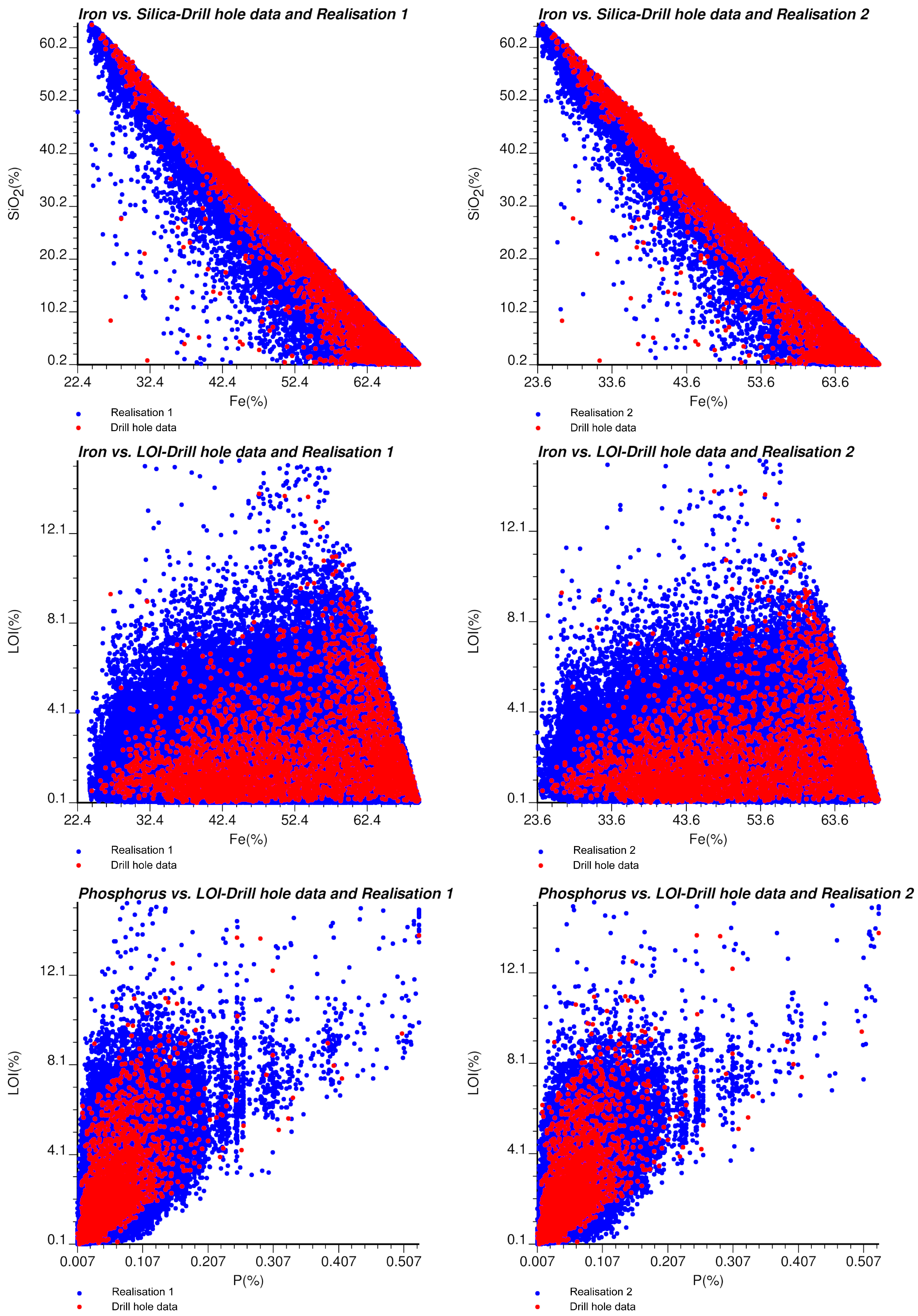
Figure 5.
Scatter diagrams of Fe vs. SiO2, Fe vs. LOI, and LOI vs. P for drill hole data (red) and simulated values (blue). Left: realisation 1, right: realisation 2.
Figure 5.
Scatter diagrams of Fe vs. SiO2, Fe vs. LOI, and LOI vs. P for drill hole data (red) and simulated values (blue). Left: realisation 1, right: realisation 2.
Figure 6.
Isometric view of two realisations of the classified rock type (left: realisation 1 and right: realisation 2), showing the plan view and vertical cross-sections passing through the origin (local coordinate system). Waste and air are shown in dark blue and grey, respectively.
Figure 6.
Isometric view of two realisations of the classified rock type (left: realisation 1 and right: realisation 2), showing the plan view and vertical cross-sections passing through the origin (local coordinate system). Waste and air are shown in dark blue and grey, respectively.
Figure 7.
Isometric view of block classification according to criteria in
Table 5, showing the plan view and vertical cross-sections passing through the origin (local coordinate system). Waste and air are shown in dark blue and grey, respectively.
Figure 7.
Isometric view of block classification according to criteria in
Table 5, showing the plan view and vertical cross-sections passing through the origin (local coordinate system). Waste and air are shown in dark blue and grey, respectively.
Table 1.
Associations between rock types and quantitative variables (for each variable, “poor” and “fine” refer to the rock types with the lowest values, and “rich” and “coarse” to the rock types with the highest values) [
23].
Table 1.
Associations between rock types and quantitative variables (for each variable, “poor” and “fine” refer to the rock types with the lowest values, and “rich” and “coarse” to the rock types with the highest values) [
23].
| G | Fe | SiO2 | Al2O3 | Mn | LOI | P | Rock Code |
|---|
| Coarse | Rich | Poor | | | | | 2 |
| Coarse | Poor | Rich | | | | | 6 |
| Fine | Rich | Poor | Rich | | | | 3 |
| Fine | Rich | Poor | Poor | | | | 1 |
| Fine | Intermediate | Intermediate | Rich | Rich | | | 5 |
| Fine | Intermediate | Intermediate | Rich | Poor | Rich | Rich | 9 |
| Fine | Intermediate | Intermediate | Rich | Poor | Poor | Poor | 4 |
| Fine | Intermediate | Intermediate | Poor | | | | 8 |
| Fine | Poor | Rich | | | | | 7 |
| Intermediate | Rich | Poor | Rich | Poor | Rich | | 10 |
Table 2.
Correlation coefficients of drill hole data and simulated outcomes of grades and granulometry (correlation observed on drill hole data: bold entries above main diagonal; average correlation over 20 outcomes: regular entries above main diagonal; minimum correlation over 20 outcomes: bold entries under main diagonal; maximum correlation over 20 outcomes: regular entries under main diagonal).
| Variable | Fe | Si | P | Al | Mn | LOI | G |
|---|
| Fe | 1 | −0.98/−0.99 | 0.21/0.18 | 0.27/0.30 | −0.04/−0.01 | 0.23/0.23 | −0.11/−0.07 |
| Si | −0.99/−0.98 | 1 | −0.30/−0.29 | −0.39/−0.42 | −0.08/−0.08 | −0.36/−0.37 | 0.14/0.11 |
| P | 0.14/0.22 | −0.32/−0.25 | 1 | 0.33/0.43 | 0.11/0.16 | 0.72/0.73 | −0.07/−0.10 |
| Al | 0.27/0.32 | −0.44/−0.39 | 0.41/0.45 | 1 | 0.19/0.17 | 0.59/0.62 | −0.38/−0.32 |
| Mn | −0.03/0.02 | −0.10/−0.06 | 0.13/0.20 | 0.14/0.21 | 1 | 0.19/0.15 | −0.06/−0.08 |
| LOI | 0.20/0.27 | −0.40/−0.35 | 0.71/0.75 | 0.60/0.64 | 0.12/0.19 | 1 | −0.18/−0.13 |
| G | −0.12/−0.04 | 0.07/0.16 | −0.14/−0.08 | −0.34/−0.30 | −0.10/−0.05 | −0.17/−0.10 | 1 |
Table 3.
Classifiers tested for the case study with their rates of correct classification on drill hole data.
Table 3.
Classifiers tested for the case study with their rates of correct classification on drill hole data.
| Classification Algorithm | Algorithm Type | Correct Classification Rate (Cross-Validation) |
|---|
| Simple Cart | Decision tree | 82.6 |
| BF Tree | Decision tree | 81.7 |
| Classification via Regression | Meta-learning algorithm | 81.7 |
| REP Tree | Decision tree | 81.6 |
| Random Forest | Decision tree | 81.1 |
| Multilayer Perceptron (Neural Network) | Function | 80.6 |
| Bayes Network | Bayesian | 77.5 |
| RBF Network | Function | 75.1 |
| Naive Bayes | Bayesian | 73.3 |
| Random Tree | Decision tree | 70.6 |
Table 4.
Prior probability of each rock type.
Table 4.
Prior probability of each rock type.
| Symbol | Rock Type Code | Prior Probability |
|---|
| p1 | 1 | 0.023 |
| p2 | 2 | 0.051 |
| p3 | 3 | 0.003 |
| p4 | 4 | 0.048 |
| p5 | 5 | 0.025 |
| p6 | 6 | 0.345 |
| p7 | 7 | 0.384 |
| p8 | 8 | 0.090 |
| p9 | 9 | 0.031 |
Table 5.
Defined conditions.
Table 5.
Defined conditions.
| Symbol | Condition |
|---|
| +1 | Block under consideration is not affected significantly by the drill hole data |
| +2 | Prior probability of the rock type interpreted by the geologists is lower than its posterior probability (the interpreted rock type “agrees” with the posterior distribution) |
| +3 | Block under consideration does not meet condition +2, but there is not any evidence for a misinterpretation (neither +4 nor +5) |
| +4 | Prior probability of the rock type interpreted by the geologists is greater than its posterior probability, posterior probability of the interpreted rock type is less than 0.15 (unlikely), and another rock type has a higher posterior probability |
| +5 | In addition to the criteria of condition +4, a rock type with higher posterior probability has been logged at some drill hole sample less than 60 m from the block |
Table 6.
Numbers of blocks with no evidence of misinterpretation (conditions +1 to +4) (diagonal line) and numbers of potentially misinterpreted blocks (condition +5) (off-diagonal) for each interpreted rock type (row) and each suggested rock type based on classification of 20 realisations (column).
| Rock Type | 1 | 2 | 3 | 4 | 5 | 6 | 7 | 8 | 9 |
|---|
| 1 | 12,058 | 35 | 51 | 22 | 35 | 21 | 76 | 61 | 29 |
| 2 | 198 | 7712 | 45 | 14 | 8 | 41 | 239 | 223 | 27 |
| 3 | 70 | 61 | 5289 | 26 | 22 | 5 | 41 | 55 | 14 |
| 4 | 93 | 39 | 99 | 15,917 | 22 | 6 | 99 | 78 | 70 |
| 5 | 96 | 15 | 38 | 55 | 5788 | 3 | 85 | 89 | 4 |
| 6 | 535 | 216 | 73 | 410 | 165 | 349,723 | 2607 | 415 | 619 |
| 7 | 2292 | 990 | 1169 | 1458 | 776 | 1161 | 172,299 | 1623 | 2072 |
| 8 | 369 | 172 | 336 | 149 | 110 | 72 | 403 | 18,259 | 233 |
| 9 | 50 | 48 | 32 | 36 | 15 | 8 | 46 | 29 | 11,875 |
Table 7.
Simulated grades and granulometry, and associated rock type, for 20 realisations of block n°1, interpreted as rock type 6 (compact itabirite) by mining geologists.
Table 7.
Simulated grades and granulometry, and associated rock type, for 20 realisations of block n°1, interpreted as rock type 6 (compact itabirite) by mining geologists.
| Realisation | Fe | SiO2 | P | Al2O3 | Mn | LOI | G | Classified Rock Type |
|---|
| 1 | 47.22 | 30.21 | 0.019 | 1.411 | 0.026 | 0.798 | 55.92 | 6 |
| 2 | 40.56 | 40.97 | 0.017 | 0.418 | 0.011 | 0.566 | 20.90 | 7 |
| 3 | 35.79 | 47.56 | 0.017 | 0.678 | 0.010 | 0.533 | 16.69 | 7 |
| 4 | 39.74 | 41.97 | 0.022 | 0.540 | 0.010 | 0.613 | 40.73 | 7 |
| 5 | 36.71 | 46.70 | 0.010 | 0.416 | 0.010 | 0.368 | 23.99 | 7 |
| 6 | 37.02 | 46.01 | 0.016 | 0.451 | 0.010 | 0.573 | 11.24 | 7 |
| 7 | 41.50 | 38.96 | 0.017 | 0.536 | 0.020 | 1.113 | 32.39 | 7 |
| 8 | 59.11 | 14.72 | 0.010 | 0.384 | 0.010 | 0.343 | 10.60 | 8 |
| 9 | 52.29 | 20.23 | 0.072 | 1.703 | 0.029 | 3.113 | 31.50 | 8 |
| 10 | 38.68 | 44.03 | 0.012 | 0.330 | 0.010 | 0.301 | 49.71 | 7 |
| 11 | 37.93 | 43.16 | 0.036 | 0.570 | 0.010 | 1.950 | 43.22 | 7 |
| 12 | 37.42 | 45.59 | 0.010 | 0.311 | 0.010 | 0.570 | 37.23 | 7 |
| 13 | 30.67 | 55.29 | 0.014 | 0.320 | 0.010 | 0.502 | 14.52 | 7 |
| 14 | 32.97 | 52.01 | 0.011 | 0.254 | 0.010 | 0.563 | 42.12 | 7 |
| 15 | 30.54 | 54.77 | 0.012 | 0.702 | 0.010 | 0.814 | 34.56 | 7 |
| 16 | 44.76 | 33.78 | 0.017 | 1.146 | 0.027 | 1.013 | 16.65 | 7 |
| 17 | 45.96 | 32.21 | 0.017 | 0.988 | 0.014 | 1.032 | 33.37 | 7 |
| 18 | 40.43 | 41.54 | 0.013 | 0.303 | 0.010 | 0.314 | 45.39 | 7 |
| 19 | 47.19 | 30.01 | 0.032 | 1.164 | 0.018 | 1.263 | 41.08 | 7 |
| 20 | 42.17 | 37.34 | 0.048 | 0.901 | 0.015 | 1.343 | 44.33 | 7 |
Table 8.
Simulated grades and granulometry, and associated rock type, for 20 realisations of block n°2, interpreted as rock type 7 (friable iron-poor itabirite) by mining geologists.
Table 8.
Simulated grades and granulometry, and associated rock type, for 20 realisations of block n°2, interpreted as rock type 7 (friable iron-poor itabirite) by mining geologists.
| Realisation | Fe | SiO2 | P | Al2O3 | Mn | LOI | G | Classified Rock Type |
|---|
| 1 | 67.59 | 1.07 | 0.013 | 1.193 | 0.010 | 1.054 | 26.67 | 1 |
| 2 | 66.88 | 2.50 | 0.016 | 1.240 | 0.010 | 0.584 | 46.37 | 1 |
| 3 | 66.17 | 3.46 | 0.015 | 1.275 | 0.010 | 0.613 | 48.08 | 1 |
| 4 | 64.99 | 5.14 | 0.014 | 1.317 | 0.010 | 0.576 | 3.89 | 1 |
| 5 | 67.46 | 1.68 | 0.018 | 1.020 | 0.010 | 0.805 | 19.45 | 1 |
| 6 | 68.66 | 1.24 | 0.010 | 0.346 | 0.010 | 0.216 | 57.84 | 2 |
| 7 | 62.30 | 7.40 | 0.015 | 2.319 | 0.010 | 1.161 | 10.35 | 1 |
| 8 | 66.55 | 2.07 | 0.020 | 1.663 | 0.010 | 1.061 | 25.53 | 1 |
| 9 | 67.89 | 2.27 | 0.010 | 0.361 | 0.010 | 0.272 | 2.92 | 1 |
| 10 | 68.74 | 0.83 | 0.015 | 0.388 | 0.010 | 0.448 | 31.09 | 1 |
| 11 | 62.57 | 9.15 | 0.012 | 0.851 | 0.010 | 0.503 | 10.12 | 1 |
| 12 | 61.69 | 9.59 | 0.024 | 0.970 | 0.010 | 1.168 | 18.37 | 8 |
| 13 | 65.41 | 3.59 | 0.016 | 1.816 | 0.010 | 1.021 | 35.01 | 1 |
| 14 | 67.70 | 2.10 | 0.012 | 0.679 | 0.010 | 0.389 | 10.40 | 1 |
| 15 | 67.63 | 0.65 | 0.028 | 1.240 | 0.011 | 1.339 | 37.19 | 1 |
| 16 | 67.66 | 1.84 | 0.021 | 0.704 | 0.010 | 0.659 | 14.63 | 1 |
| 17 | 59.19 | 14.67 | 0.010 | 0.397 | 0.010 | 0.272 | 1.93 | 8 |
| 18 | 62.59 | 8.48 | 0.012 | 1.255 | 0.010 | 0.743 | 22.11 | 1 |
| 19 | 66.79 | 1.55 | 0.032 | 1.533 | 0.016 | 1.338 | 31.18 | 1 |
| 20 | 68.48 | 0.71 | 0.016 | 0.581 | 0.010 | 0.748 | 32.40 | 1 |
Table 9.
Simulated grades and granulometry, and associated rock type, for 20 realisations of block n°3, interpreted as rock type 8 (friable iron-rich itabirite) by mining geologists.
Table 9.
Simulated grades and granulometry, and associated rock type, for 20 realisations of block n°3, interpreted as rock type 8 (friable iron-rich itabirite) by mining geologists.
| Realisation | Fe | SiO2 | P | Al2O3 | Mn | LOI | G | Classified Rock Type |
|---|
| 1 | 63.608 | 0.80 | 0.052 | 0.873 | 0.410 | 6.736 | 9.90 | 3 |
| 2 | 62.235 | 2.79 | 0.076 | 3.258 | 0.021 | 4.770 | 14.71 | 3 |
| 3 | 62.653 | 1.17 | 0.042 | 1.497 | 0.053 | 7.595 | 4.63 | 3 |
| 4 | 64.02 | 2.96 | 0.037 | 2.453 | 0.064 | 2.884 | 1.80 | 1 |
| 5 | 64.817 | 0.80 | 0.095 | 1.886 | 0.095 | 4.310 | 20.67 | 3 |
| 6 | 62.642 | 2.64 | 0.105 | 3.058 | 0.083 | 4.397 | 14.68 | 3 |
| 7 | 63.305 | 1.23 | 0.047 | 2.737 | 0.073 | 5.326 | 34.15 | 3 |
| 8 | 62.068 | 1.11 | 0.126 | 3.221 | 0.034 | 6.600 | 21.30 | 3 |
| 9 | 65.543 | 0.39 | 0.069 | 1.635 | 0.031 | 4.065 | 23.33 | 3 |
| 10 | 62.09 | 0.97 | 0.070 | 2.925 | 0.095 | 7.048 | 44.50 | 3 |
| 11 | 63.943 | 1.32 | 0.037 | 1.387 | 0.024 | 5.758 | 32.72 | 3 |
| 12 | 63.108 | 1.14 | 0.039 | 2.357 | 0.039 | 6.141 | 7.71 | 3 |
| 13 | 59.538 | 2.04 | 0.073 | 6.104 | 0.080 | 6.466 | 8.94 | 9 |
| 14 | 62.418 | 0.52 | 0.099 | 3.669 | 0.075 | 6.244 | 5.13 | 3 |
| 15 | 62.12 | 0.41 | 0.096 | 3.155 | 0.033 | 7.361 | 6.21 | 3 |
| 16 | 63.739 | 0.52 | 0.040 | 1.420 | 0.148 | 6.644 | 23.91 | 3 |
| 17 | 57.725 | 0.49 | 0.095 | 5.816 | 3.110 | 6.932 | 11.19 | 5 |
| 18 | 64.591 | 1.03 | 0.067 | 1.721 | 0.033 | 4.707 | 17.59 | 3 |
| 19 | 62.706 | 2.49 | 0.079 | 2.092 | 0.018 | 5.559 | 21.10 | 3 |
| 20 | 64.873 | 0.57 | 0.043 | 1.131 | 0.025 | 5.423 | 40.42 | 3 |
© 2017 by the authors. Licensee MDPI, Basel, Switzerland. This article is an open access article distributed under the terms and conditions of the Creative Commons Attribution (CC BY) license (http://creativecommons.org/licenses/by/4.0/).


