Article

Nano-Tomography of Porous Geological Materials Using Focused Ion Beam-Scanning Electron Microscopy

1
Debye Institute for Nanomaterials Science, Utrecht University, Princetonplein 1, 3584 CC Utrecht, The Netherlands
2
Department of Earth Sciences, Utrecht University, Budapestlaan 4, 3584 CD Utrecht, The Netherlands
*
Authors to whom correspondence should be addressed.
Minerals 2016, 6(4), 104; https://doi.org/10.3390/min6040104
Submission received: 18 July 2016 / Revised: 23 September 2016 / Accepted: 28 September 2016 / Published: 10 October 2016
(This article belongs to the Special Issue Advances in Mineral Analytical Techniques)

Abstract

:
Tomographic analysis using focused ion beam-scanning electron microscopy (FIB-SEM) provides three-dimensional information about solid materials with a resolution of a few nanometres and thus bridges the gap between X-ray and transmission electron microscopic tomography techniques. This contribution serves as an introduction and overview of FIB-SEM tomography applied to porous materials. Using two different porous Earth materials, a diatomite specimen, and an experimentally produced amorphous silica layer on olivine, we discuss the experimental setup of FIB-SEM tomography. We then focus on image processing procedures, including image alignment, correction, and segmentation to finally result in a three-dimensional, quantified pore network representation of the two example materials. To each image processing step we consider potential issues, such as imaging the back of pore walls, and the generation of image artefacts through the application of processing algorithms. We conclude that there is no single image processing recipe; processing steps need to be decided on a case-by-case study.

1. Introduction

The focused ion beam (FIB) instrument was first developed for machining devices at a micrometre or sub-micrometre scale and as a method for preparing samples of various shapes [1,2,3,4,5,6]. However, the instrumentation has gradually been adapted to produce electron-transparent thin sections (foils) of biological samples, usually between 50 and 250 nm thick, for transmission electron microscopy (TEM) observations in two dimensions (2D) and also in three dimensions (3D) through tomographic acquisition [7,8]. This tradition of sample preparation in FIB has been extended into materials sciences [9,10,11], not only for simple planar foils but also for more complex shapes such as conical or cylinder forms required for optimizing scanning (S)TEM tomography and atom probe tomography (APT) [12,13]. Over the last few decades, the FIB unit was further developed to include an ion beam gun coupled with a scanning electron microscope (SEM) column into a dual-beam or double-column system also known as FIB-SEM [14,15,16]. The great advantage of combining SEM and FIB is that SEM imaging allows for precise selection of an area of particular interest (such as an interface or grain boundary) that can then be analysed in 3D by means of FIB preparation [17,18,19,20,21,22,23]. This is nowadays routinely performed in the semiconductor industry to investigate the performance of devices [24]. In addition to traditional biological and materials sciences [25,26,27,28,29,30,31,32,33], FIB-SEM analysis of natural solid materials, e.g., geological materials, has recently become increasingly popular [34,35,36,37].
‘Tomography’ is the acquisition and visualization of slices or sections of a material to generate a 3D image of that material. This can be achieved using the dual-beam systems, where imaging and slicing are directly correlated creating a FIB-SEM cross section series [15,38]. Performing such 3D acquisitions on porous materials can resolve mesopores and macropores [39], and characterize the interactions between them. Understanding these features provides essential information about the formation mechanism and the transport properties of such materials [40,41]. Many examples are directly relevant to industrial use, where the study of transport properties is essential to facilitate the recovery of oil and gas contained in reservoir rocks [42,43,44]. FIB-tomography can provide such 3D data down to nanometre-scale resolution within a representative volume. Due to FIB-SEM capabilities, the technique can be applied to a large variety of materials [38]. The most challenging aspect of using FIB-SEM for such 3D tomography is the treatment of the data, i.e., slice image stack, to produce representative reconstructions. This is a particularly important challenge for porous materials, where the porosity and size distribution of the pores are unknown prior to analysis, which makes the accuracy of the segmentation procedure of the internal microstructures difficult to evaluate [45,46,47,48,49]. Until now, there has still been no benchmark of the precision of the segmentation procedure, which is influenced by artefacts introduced by negative interactions between the beams and the material into the slice images during 3D acquisition. Thus, the final result is dependent on the instrument operator. This information is fed directly into further analysis of pores, pore network verification (connectivity), and area and volume calculation; therefore, the effects of different segmentation procedures have a direct impact on the final results. In this paper we discuss the methodology of FIB-SEM tomography and give an account of its benefits and limitations, in particular from the point of view of the characterization of porous geological materials. Two different examples from geologically relevant samples are used to demonstrate the FIB-SEM serial sectioning procedure and analytical choices. Both example materials are siliceous in nature and therefore have similar properties in SEM images.
The first example material is a natural diatomite rock sample (Figure 1) from a Tripoli diatomite formation (Sicily, Italy). Diatomite, also referred to as diatomaceous earth, is a fragile rock that consists of loosely bound fossilized unicellular diatom algae [50]. As a consequence, this material has high porosity and thus high permeability, high surface area, and low density. These properties make this material particularly interesting as a heavy metal adsorbant for contaminant removal [51] and for catalysis e.g., for the generation of phenol [52], as a catalytic substrate [53]. All these process are dependent on the interconnectivity of the porosity and accessibility of the surface area, thus 3D visualization can provide a wealth of information about how gases and liquids can permeate these materials. Due to the small size of the pore space and complex internal structure, FIB-SEM tomography is an optimal method for examining this material. The second example material is amorphous silica, produced through the experimental reaction of olivine (Mg0.8Fe0.2SiO4) with an acidic solution (Figure 2). Olivine is an interesting input material for a lot of different industrial processes including the neutralization of highly acidic fluids and industrial CO2 sequestration [54,55,56]. The experimental procedure and chemical analysis of the material can be found in [56]. The formation and properties of newly precipitated material on olivine surfaces will control further reactivity as it will mediate the ability of reactive fluid species to access the reacting interface [57,58]. Reaction of olivine produced an amorphous silica pseudomorph around the original olivine grain that appeared to be layered from 2D electron microscopy imaging. The layering in reacted silica shows a discrete separation with high porosity. Despite both of these materials being silica-rich, the two materials show distinctly different porosity characteristics and require different treatments both during the tomographic procedure as well as post-acquisition data treatment.

2. Concept of FIB-SEM

2.1. Microscope

A typical FIB-SEM system (see examples in Figure 3a) consists of a field emission gun that discharges electrons into a vertical column to be focused onto the sample surface, a liquid metal ion source (LMIS) within an inclined ion beam column (typically 52° from the SEM column axis, however, this varies depending on the manufacturer), and a gas injection system (GIS). Different gases can be used depending on the requirements of the sample. For geological samples, platinum combined with an organic molecule to produce a gaseous phase is most often chosen due to its action as a welding material. More advanced systems are also equipped with standard SEM devices such as Energy-dispersive X-ray spectroscopy (EDX) detectors for chemical analysis and Electron backscatter diffraction (EBSD) cameras for crystallographic characterization. Nano-manipulators are also a common feature of these systems as they provide nanometre control of sample positioning, which is especially helpful for TEM foil preparation and other operations such as nano-machining and handling nano-sized objects (Figure 3c).
Imaging of samples is conducted using a variety of different detectors including ETDs (Everhart–Thornley detector), TLDs (through lens detector) producing SE (secondary electrons) and BSE (backscattered electrons) images, and CL (cathodoluminescence) detectors for imaging luminescent material, thanks to the large sample chamber capacity (Figure 3b). For geological samples CL can be particularly interesting as it provides information about chemical zoning related to growth and deformation, allowing alternative methods for area of interest identification. State-of-the-art detectors, such as those in the FEI (field electron and ion) Helios FIB-SEM system (Figure 3d), include MD (mirror detector), ICD (in-chamber detector), retractable CBS (concentric BSE detector) for BSE images recording, and a retractable STEM (scanning transmission electron microscopy) detector that can produce low-voltage imaging with transmitted electrons through, for instance, a prepared thin foil.

2.2. Tomography Setup

Sample preparation prior to insertion into the FIB-SEM is analogous to that used for typical SEM analysis. The sample must be prepared in such a manner that it can be attached to the sample stage. If the sample is in chip or powder form this typically consists of attaching the sample to a SEM stub using conductive carbon tape or silver glue. Typical geological thin sections can either be inserted directly using a specialized holder or mounted on a stub depending on the instrument manufacturer. As most geological materials have a low electrical conductivity, a thin conductive layer consisting of a few nanometres of Au, C, or Pt is deposited onto the entire sample surface. This coating procedure helps to remove electrons from the area viewed by the incident electron beam, reducing surface charging effects that interfere with the backscattered and secondary electrons emitted by the sample. In addition, the coating protects the material from being degraded during imaging using the more destructive ion beam. The carbon tape or silver glue should also be used at the sample sides to create a bridge between the surface of the material and the stub, further improving the charge conduction from the top surface.
After a sample is prepared and mounted into the chamber stage, the tomography procedure can be carried out as illustrated in Figure 4a.
Within the instrument itself, the sample is first analysed with the electron beam to find an area of interest. As in a conventional SEM, the electron beam of the FIB-SEM system arrives at the surface of the sample perpendicularly. However, the angular difference (i.e., 52°) between the FIB and vertical SEM columns means that the incident ion beam will not interact with the surface in a perpendicular manner in the original loading orientation; thus, the sample must be inclined to 52° prior to a typical tomography acquisition, as can be seen in Figure 4b.
After tilting, the sample stage is adjusted to the coincidence position at the eucentric height for both columns, meaning that both the ion and electron beams are focused on exactly the same point at the sample surface. To protect the selected region of interest (ROI) from damage during the long tomographic process of ion imaging and milling, a layer of Pt with a thickness around 1 µm is deposited on the surface using the GIS system with assistance from the FIB. The area surrounding the ROI protected by Pt is then milled using the ion beam to produce a ‘U’ form cavity. In this way, the area to be imaged is isolated from the surrounding sample material, lowering the chances that milled matter can redeposit on the sample face. The size of the cube, in the slicing direction, should be equal to the selected slice thickness multiplied by the number of images to be generated in the imaging plane of the cross section. Critically, the width in the X dimension of the imaging plane should be determined according to a compromise between the anticipated pixel size, as defined by the scanning step of the electron beam, and the resolution of the slice image expected to be recorded.
Once the preparation of the isolated cube is complete, the free face of the cube perpendicular to the sample surface is gently ‘polished’ using a low ion current [4,59,60]. Polishing produces a smooth, flat surface for imaging and, along with the presence of the protective Pt surface layer, reduces the curtaining effect, producing the most accurate electron image of the material [61,62]. The curtaining effect, as can be seen in Figure 5, relates to the formation of stripes parallel to the FIB milling direction on the cross section. This results in a roughness within the slice plane and thus slice milling with inconsistent thickness. This is particularly the case when the sample surface has a rough topography or the material contains phases with different densities [60,63]. This effect is greatly reduced by depositing a thick Pt layer on the top surface above the ROI by in situ FIB assisted deposition, followed by gentle ion milling (polishing using a relatively low ion beam). The polishing will also eliminate redeposited amorphous material on the cross section face, which occurs during the U-cavity milling. Redeposition is limited by creating a U cavity that is large enough for the milled matter to escape. This is also critical to reduce the amount of redeposition during the tomographic acquisition, which can block the field of view of the slicing plane.
Subsequent to polishing, the instrument is set up to run a serial sectioning sequence using experimental parameters that have been optimized for the sample analysed, such as scanning speed, imaging mode, etc. This includes the slice thickness, i.e., the amount of material to be milled away by the ion beam prior to imaging the surface. The slice thickness is determined based on the size of the target objects to be revealed in 3D, where the size of the smallest object should be larger than the slice thickness (and pixel size in the images). If they are smaller than the slice, some could be missed during slicing, thus not producing a representative 3D volume reconstruction. Another influencing factor is the interaction volume of the electron beam within the sample at different acceleration voltages, which will have consequences for electron imaging. For example, in the diatomite sample discussed here, Monte Carlo simulations indicate that BSEs (red trajectories in Figure 6) generated through interaction of the siliceous material with a 2 kV incident electron beam at a 38° angle are not produced deeper than 20 nm into the sample. Therefore, a step size of not more than 20 nm should be used in order to record all the information within the area of interest. Before performing a tomographic procedure, the optimal imaging conditions also need to be determined based on the electron beam acceleration voltage, imaging mode, dwell time, etc. Figure 5 shows two images of a polished cross section from the ROI chosen for the reacted olivine sample. As can be seen in Figure 5, at the same beam acceleration voltage the BSE image provides more contrast between the pores and the material and is less sensitive to charging effects. If multiple detectors are available these should be tested in the same imaging mode to verify which one provides the highest quality image.
The serial sectioning procedure itself occurs in three steps: (1) the ion beam mills away a thin layer at a current similar to the one used for polishing; (2) the focus of the electron beam is automatically adjusted based on the working distance (WD) variation that is related to the thickness of the slice erased during the milling; and (3) a SEM image is recorded from the newly uncovered material on the face of the cube. Once the imaging is finished, the instrument begins again, running the sequence repeatedly until the preset number of steps has been reached. Each slice image consists of a certain number of voxels (3D pixels), each representing a volume of the material. However, each voxel is in general not isotropic. In the XY plane, which should be described as XY´ because the recorded image is actually a projection of the inclined cross section, the voxel size is defined by the pixel size, which is linked to the magnification or numerical resolution of the SEM images. In contrast, in the Z direction the voxel size is defined by the expected constant thickness of the slices removed by FIB milling. Thus, typically, the voxel size in Z is larger than the XY pixel size. As discussed above during a tomographic procedure, the sample is inclined at 52° to the electron beam with the ion beam perpendicular to the sample surface. Thus the imaged section has an angle of 38° with the incident electron beam and the generated electron images of the section have an angular issue cos(38°) to the normal vertical projections. This only affects the Y dimension and the real length in the inclined section plane can be directly related to the length in the projection image by dividing the length by cos(38°). This correction can be performed in two ways: (1) automatic correction by the microscope control program; (2) numeric correction after acquisition using software such as ImageJ (https://imagej.nih.gov/ij/) and Fiji (a distribution of ImageJ, http://fiji.sc/) [64,65], and FEI Avizo (http://www.fei.com/software/avizo-3d-for-materials-science/). Due to this issue, the ‘Dynamic focus’ function of the SEM should be activated during serial sectioning, which adapts the focal point of the beam on the tilted plane to compensate for different WDs along the Y direction, producing a correctly focused image across the field of view.

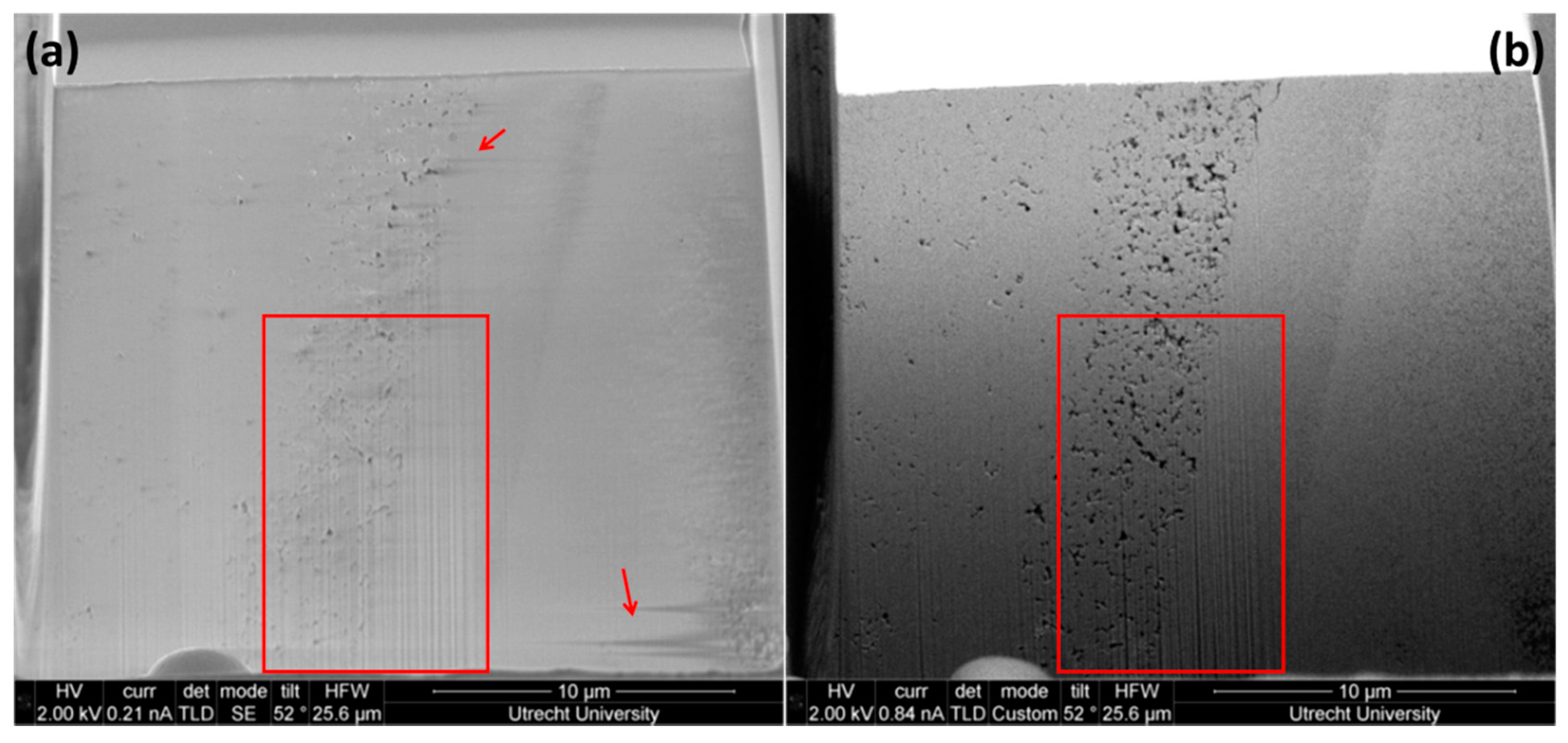
2.3. Instrument Setup to Limit Artefacts during Sample Analysis
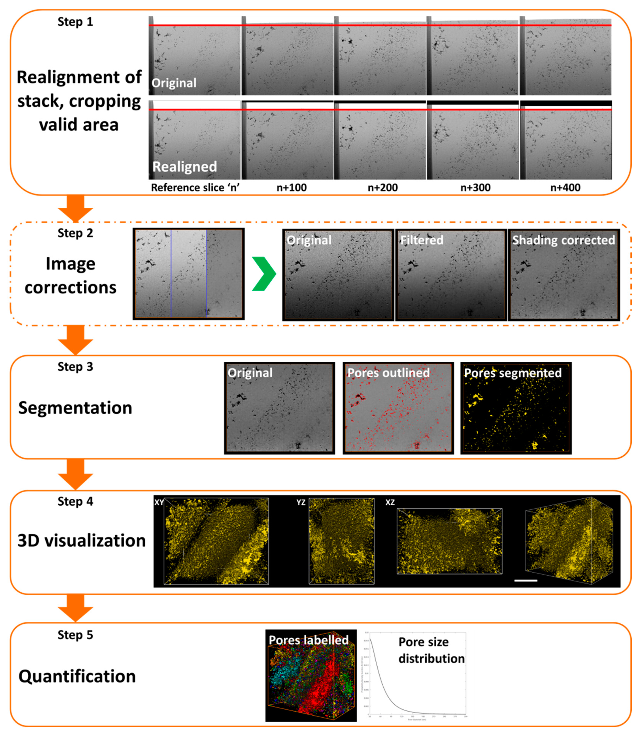
Creation of the U cavity around the ROI has the added benefit of reducing shadowing effects. This is illustrated in Figure 5b as a systematic reduction in brightness from the top to bottom of the cross section image in the Y direction. It is particularly pronounced when BSE imaging is used, thus for porous materials, where BSE gives a better contrast between pores and the surrounding material, efforts to limit this effect should be taken. Shadowing is caused by an increase in obstacles along the signal electron trajectories in the lower part of the section. The dominant cause of this is interactions with the walls of the U cavity that isolate the ROI. Thus creation of a large enough cavity around the area to be imaged will reduce the shadowing effect on the front cross section plane. The practical way to avoid this issue is by milling a large cavity around the ROI to provide the electrons with enough free space to escape the trench. However, erasing a very large volume takes time, especially in hard and poorly conductive materials or when a large cross section is needed. Thus a compromise between the pit size and later numerical treatment of the shadowing effect during data reduction is used. In the two samples studied in this article, pits of 40 × 30 and 50 × 25 µm2 were created in the diatomite and amorphous silica samples, respectively. In the diatomite sample (Figure 1b) the shadowing effect is less pronounced than in the amorphous silica sample in Figure 5b due to the different distances between the cross section plane and the opposite wall of the U cavity.
A common phenomenon in the analysis of geological materials is electron charging due to the inefficient transport of electrons away from the incident beam location. This creates high contrast areas within the electron images that are unrelated to internal structures and must be reduced prior to running a tomographic series acquisition to be able to accurately reconstruct the data during image analysis. Although this effect is mediated at the sample surface through the application of a conductive film as described above, the freshly milled surfaces created through the tomographic procedure are not coated. Therefore, charging of the milled face can be a problem, particularly for highly porous materials where edge charging effects are evident. To combat this, low beam currents are used to perform the electron imaging between each milling section, limiting the intensity of the incoming electrons at the sample surface. For example, for both the insulating materials described here an acceleration voltage of 2 kV and probe current of 0.84 nA were required to produce acceptable electron images. A summary of the conditions used in the two FIB-SEM tomography examples for the studied samples can be found in Table 1.
The use of a high-intensity ion beam to mill the material can also lead to implantation of the ions into the studied material, which in turn produces surface defects and topography changes. Similar effects can occur during FIB imaging and in situ deposition using the GIS. To minimize this, the top sample surface is protected by the previously sputtered metal coating during the location procedure for ROI, which in our case is a Pt coating up to 15 nm. This is sufficient to avoid electron beam charging and damage, even for non-conductive materials. The interaction volume between Ga and the material is much smaller than that of electrons; the ions accelerated by a 30 kV voltage can penetrate tens of nanometres into the surface compared to microns for electrons with the same acceleration voltage [67,68]. Thus, for ion beam imaging and slice milling, a Pt-layer of about 1 µm deposited in situ was made to protect the ROI. In addition, a low beam current should be applied to reduce the ion dose [69]. During serial sectioning the newly made cross section is not protected by any coating or deposition layers. However, as the cross section plane is parallel to the FIB incident direction, the ion contamination into the section plane is related directly to the sputtering of ions during former slice milling, and is limited due to the small contact angle.

3. Image Processing

After acquisition of the slice images, the data are reconstructed into a 3D volume using the steps described in Figure 7. This can be summarized into four tasks: (1) realigning the images; (2) correcting for instrument based artefacts; (3) segmentation; and (4) visualization. In general, the large number of files and sophisticated data analysis algorithms require the use of specialist software packages and computer systems. For the analysis of the samples described in this article the freeware program Fiji [36] was used in conjunction with the commercially available FEI Avizo program. The main difference between these programs lies in their data analysis capabilities, with Avizo providing professional quantification and visualization tools specifically designed for tomography applications.

3.1. Realignment of Image Stack

At the end of the FIB-SEM tomography experiment, we obtain a series of several hundred to thousands of images. This stack of slice images needs no real reconstruction procedure, as is required for TEM tomography projection series. Although a fiducial marker (Figure 4b) is used in the instrument ROI relocation and WD update, slice images may still drift due to charging effects within the cross section. Thus the stack must be realigned to account for the imaging field drifts. The programs described above provide an automatic alignment algorithm without landmarks that is based on a cross correlation approach. It uses an allocated slice image as a reference, for realignment of the subsequent image. The comparison between the two consecutive images is conducted via pattern recognition based on the grey level of every pixel within the entire frame. Each newly aligned image is used as the reference for the next image until the whole slice stack has been checked. As FIB-SEM tomography does not involve any continuous tilting of the sample as in TEM tomography, the shapes of internal microstructures are not affected by projection effects. Thus, it would be expected that cross correlation alignments of FIB-SEM images should produce a simpler and better alignment compared to TEM tomography. However, the complexity and evolution of the microstructures, e.g., the pores in this study, and their visualization in 2D, means that further refinement of the realignment is required including manual correction. When the realignment is fulfilled, the black borders generated, for example those seen in realigned images in Step 1 of Figure 7, due to the translations of image area within the frame should be cut away before further treatments. This is unavoidable cropping effect reduces the valid image area. Thus this issue should be considered when deciding the size of the cross section prior to ROI identification.

3.2. Image Corrections
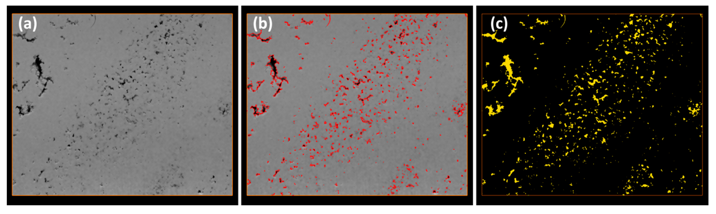
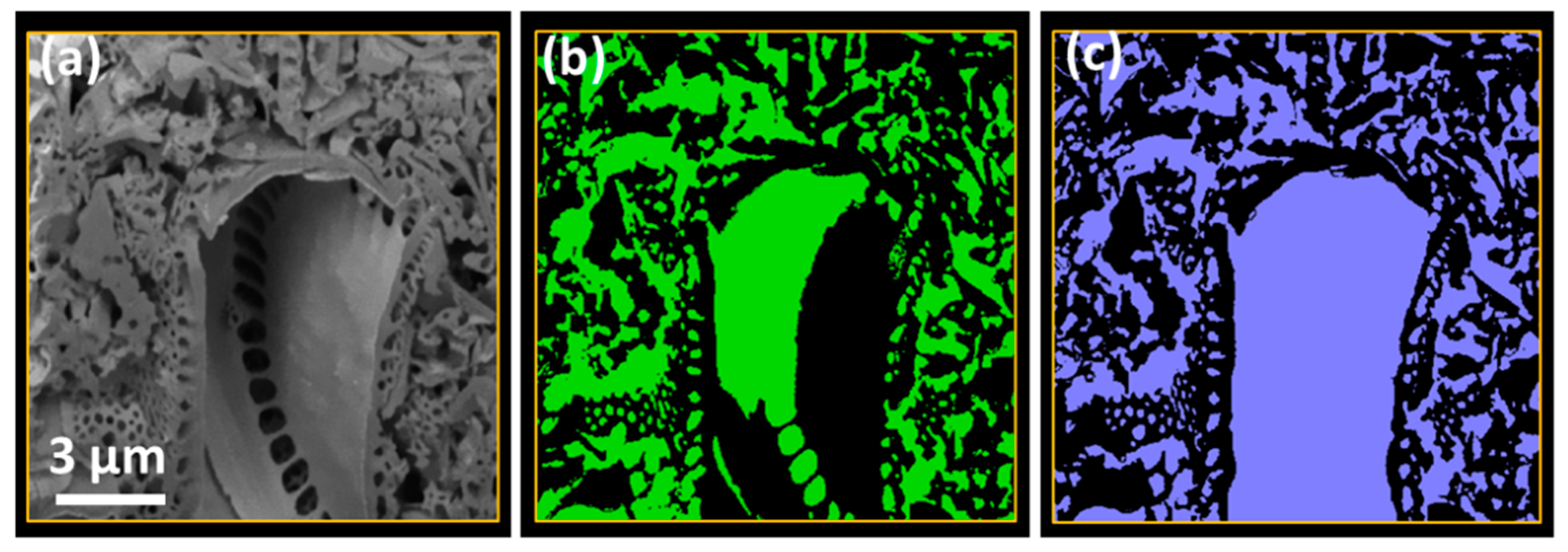
In certain cases, the slice images need post-treatment to enhance the quality and to remove artefacts caused by the FIB-SEM technique, e.g., the curtaining effect and the shadowing effect that have been discussed in Section 2.2 and Section 2.3. If those negative effects persist even with the experimental precautions, numerical corrections are used. The curtaining can be reduced by applying a fast Fourier transform (FFT) filter. However, if the stripes only appear partly within the cross section, as in the case shown in Figure 5, extra caution should be taken so as not to create new artefacts elsewhere through the use of such a filter. The shadowing can be treated numerically by normalizing contrast along the Y axis in the recorded images, shown as a result in Step 2 of Figure 7. Some images may have an excessive amount of noise caused by low voltage and probe current imaging. Smoothing of the images is conducted to remove this noise, also using filters. There are a number of different filters (Gaussian blur, mean and median, erosion, etc.) for this task and each should be tested and assessed manually to establish which one produces the best outcome for subsequent data processing. This treatment is not always necessary with current analytical capabilities, where the state-of-the-art detectors provided in high-end instruments can provide very high quality images. More importantly, each intervention of such numerical treatment alters the original images, which in turn could create other artefacts that can influence the result of further data analysis. This factor should also be considered and taken into account based on the purpose of each study.

3.3. Segmentation

The image segmentation involves separating different phases of the sample, distinguished by different contrast, in the slice images and then generating a 3D image of only the target phase. In the present study, the Avizo software was principally applied for the segmentation of the pore space (Step 3 of Figure 7). This program contains various segmentation algorithms and associated tools, so different strategies can be taken depending on the objectives of the study.
In the case of the olivine sample, image segmentation was carried out using a marker-based watershed transformation [70,71]. In this segmentation method, the grey values in a gradient image are considered to represent the height of a relief. Thus the edges between different phases within the image have a high gradient value, enclosing areas of low gradient values. Next, specific markers are defined by the operator through thresholding within different phases—in our case, the pore space on the background and the material in the imaging plane. Then the watershed transform is computed on the modified function with markers, working towards separating the pores from the material. The name watershed comes from its use of water flow simulation methodology to follow gradients within the image into areas with a local minima, in this case pore space, which are shown as the segmented phase in the resulting image. With the marker-based transformation, the over-segmentation is improved. The pores in the analysed volume have a narrow size distribution range, only this treatment is required to extract all the pores from the images. In Figure 8, a single slice from the image stack obtained from the olivine sample is shown. The pores mostly have a low grey level and thus appear as dark regions in the image. The red lines (Figure 8b) are generated by contouring the segmentation calculated for the slice, and outline the pores determined by the computer for this 2D image. Comparison of the watershed segmentation (Figure 8c) with the original image (Figure 8a) demonstrates the ability of this segmentation technique to adequately reproduce the porosity.
However, the watershed segmentation cannot recreate the pores in the diatomite sample of a single slice (Figure 1b) as the porosity varies in size between tens of nanometres and several micrometres, which is a much larger distribution than that found in the olivine sample. Segmentation is hindered in the watershed method because the back wall of larger pores below the imaging plane can produce the same contrast greyscale value in the 2D images as the surrounding solid material. Thus, during segmentation, the algorithm cannot distinguish between the pores and the surrounding material and produces an unrepresentative result. An example of such a big pore produced by an intact fossilised diatom with large internal cavity is shown as a cropped area from a single slice image in Figure 9a. During imaging the electron beam is also able to penetrate into the pore space within the diatom skeleton and interact with back pore wall due to the inclined angle of the electron beam with respect to the sliced surface. In small pores backscattered electrons have less chance of escaping from the sample as they interact with obstacles such as the surrounding material, similar to the shadowing effect described in Section 2.3. However, for large pores the BSEs generated from the back pore wall have a higher chance of escaping and adding to the backscatter contrast of the electron beam image. The effect becomes more pronounced as the back wall of the pore is approached through milling and leads to a distorted pore shape during the 3D reconstructions. Thus alternative methods must be applied to successfully segment image stacks where pore sizes are large. For the diatomite sample a grey level thresholding was first applied to the entire image stack, followed by a manual adjustment to include the large pores. The result is shown in Figure 9c and comparison with the initial image in Figure 9a indicates that this method replicates the pore space within each slice effectively without significantly increasing noise levels. Use of the different procedures makes a marked difference on the overall estimations of pore volume for interconnected pores along the slicing direction as segmentation using the watershed method over the entire slice and view area estimates these pores to occupy 25% ± 5% of the overall volume (Figure 9d), whereas the same pores are predicted to occupy 35% ± 6% with the multistage procedure (Figure 9e).

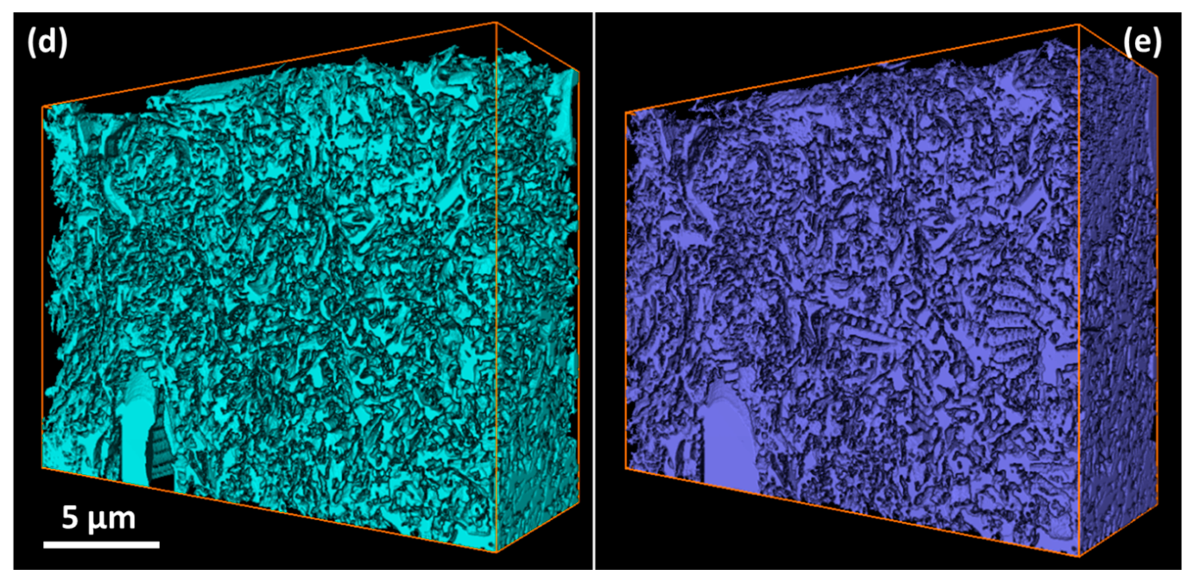
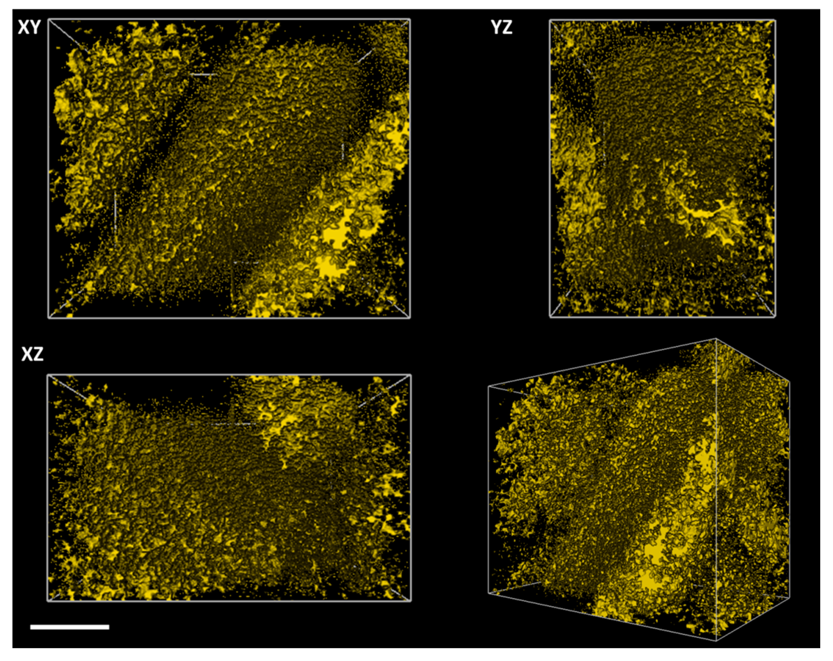
3.4. Visualization and Animation
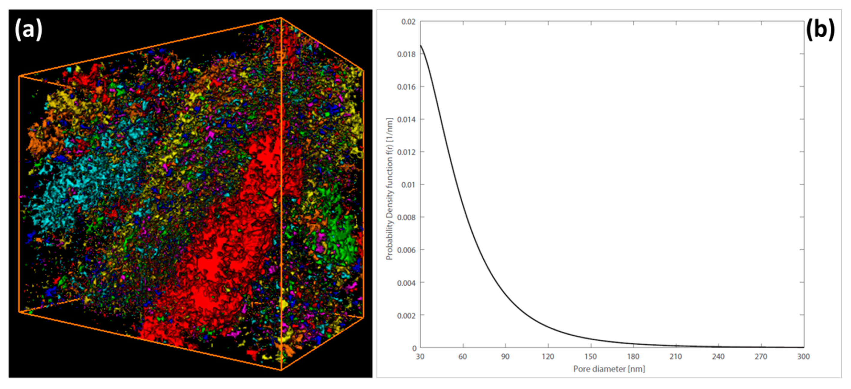
Once an accurate segmentation of the target object has been achieved, the result is visualized in 2D and 3D using the orthoslice (Figure 8) and volume rendering (Figure 10) modes in various tools of visualization, such as ImageJ/Fiji, Avizo, Imod (http://bio3d.colorado.edu/imod/), and Inspect 3D (http://www.fei.com/software/inspect-3d/), which can help us to freely check the details of the reconstructed objects including pore connectivity, shape, and size. The easiest way to visualize the tomographic result is through animations, for example the animation that can be found in the supplementary materials (Video S1) of the amorphous silica reaction product after olivine. Using these animations, the relationship between the original section images and final estimates of pore space can be demonstrated.

3.5. Quantification

One of the most powerful outcomes of tomography as an analytical tool is the ability to gain 3D, spatially connected information about volume, surface area, pore diameter, aspect ratio, etc. In 2D, estimates of these properties are difficult due to many unknown factors such as the true shape of a pore and its relationship to the cross section orientation. However, in 3D after segmentation these issues are limited and further information about pore connectivity can be traced throughout the volume examined. This in turns facilitates estimates of material permeability. This information can then be used as input parameters for numerical models to understand flow through such a pore network [72,73,74,75,76,77]. Figure 11a shows the same volume as in Figure 10, but with all the segmented pores indexed with different colours. Each pore body is painted in a colour that is different from its neighbours, with which it has no connection. A large pore body is a number of smaller pores connected together, such as the one in red in Figure 11a. The volume depicted in Figure 11 with various pore sizes was found to have no 3D interconnected pore network, meaning that no connection exists between the layered pore clusters and pores in the same cluster are also not fully connected. The continuous pore size distribution (CPSD) is indicated in Figure 11b, which illustrates that the majority of the pores are smaller than 100 nm in diameter calculated by equivalent spherical pores volumes [21]. The smallest calculated pore size is 16.5 nm of diameter, which is equivalent to the volume of one voxel and therefore likely noise. As the voxel size applied in this sample is large, the smallest calculated pores are not distinguishable from noise. This part should thus be eliminated from the final distribution.

3.6. Further Discussion

Realignment of the diatomite images was mainly carried out in the open source software Fiji. Subsequently, a volume of 1677 × 1260 × 376 voxels was retrieved. Treatments to improve the quality of the images and hence the segmentation of the pore space were performed in Avizo 9. As described, the technical difficulties associated with the overlap in the greyscale value for the large pores produce a slight underestimation of the pore space. As there is no preliminary information about the porosity, the segmentation result cannot be verified. Therefore, comparison with other techniques of porosity measurements such as mercury injection porosimetry may be an alternative in several cases to provide such information and assist in the interpretation of FIB tomography results [21,78]. Discrepancies between bulk estimations of porosity and FIB tomography can result from the random selection of the ROI in a material where the pore distribution varies in different regions, or from the invalidity of the assumptions used in the bulk estimation methods. Pore filling techniques may be a promising way to conquer the segmentation issue where inclusion of a heavy metal, which has a high contrast in BSE imaging, would greatly improve the image processing and hence the segmentation without requiring complex algorithms [79,80].
For the amorphous silica sample, a subsection of 1863 × 1539 was cropped out of the realigned stack after realignment. Thus the final volume analysed was ∼6500 µm3. Overall the pores were estimated to fill 5.29% of the total studied volume of the material. However, the 3D visualization demonstrates that the gaps clearly visible in BSE images of the entire reacted grain (Figure 10) are related to layers of porosity within the reaction rim. Within the sampled volume these layers lie parallel to one another and are separated by a layer of amorphous silica characterized by a low porosity. Within the low porosity layers there is also limited pore connectivity, indicating that there will be limited interaction of the bulk solution in the experiment and the solution at reacting interface during this interface-coupled dissolution–reprecipitation reaction. The layered structure is hypothesized to be due to areas of different silica density within the sample rim that become separated during maturation of the gel-like material originally formed or washing and drying during sample preparation. Both of these mechanisms should not significantly decrease the final porosity; rather, the formation of nanoparticles, as described in [56], would be expected to increase the porosity. The limited porosity observed with the FIB-SEM thus indicates that such silica rims should eventually retard olivine reaction with acidic solutions as they will limit the replenishment of acidity to the reacting interface.

4. Conclusions

Nano-tomography applied through the use of FIB-SEM microscopes is a powerful analytical tool that is being increasingly applied to biological [81], material [82,83], and geological problems [37,84,85,86,87]. Specifically, the integration of FIB capabilities into a typical SEM allows for the removal of material with a high spatial control and precision to generate images of the freshly exposed material in situ within minutes. However, the true power of FIB-SEM is the sequential removal and imaging of material that can be reconstructed to produce 3D visualizations of complex microstructures and pore networks. The analysed volumes can be large, typically up to tens of thousands of cubic micrometres, as the main limiting factor for this analysis is instrument time [88].
Reconstruction of geological and other materials using FIB-SEM bridges the gap between other tomography techniques such as those produced using X-rays and TEM. The exact achievable resolution is sample dependent as it is related to the interaction volume of the electron beam in the Z direction and the image magnification and size of the images in the X and Y directions. The correlation between the resolution of FIB-SEM and typical pore sizes found in geological materials has resulted in FIB-SEM tomography becoming a routine technique for the analysis of these materials with a wide variety of applications. However, there are clear technical difficulties that need to be considered to produce representative and reproducible data. These include minimizing instrument-related artefacts through careful choice of experimental conditions as well as conscientious data handling. Many artefacts can be eliminated during data reduction but the overall effect on the quality of the data after multiple numerical treatments should not be ignored.
Segmentation is the most difficult aspect of data reduction and methods vary depending on the level of detail required in the study and the material itself. Currently there is no general method for segmenting pores with background features, a feature common to geological materials, and thus the user must validate the results by comparing the final estimates of porosity with that expected from different section images. Segmentation methods are being adapted to combat these issues, for example the morphological segmentation method and automatic phase segmentation method presented in [89,45,46,47,48]. 3D information on pore interconnectivities has provided modellers with first-hand information about complex materials that allows them to simulate transport properties [43,74,76,90,91], thereby gaining further knowledge of how the pore shape and interactions influence fluid flow, particularly permeability and fluid velocity. Future studies need to evaluate the impact of different segmentation strategies on numerical transport modelling and test the modelling results against experimental investigations.

Supplementary Materials

The following are available online at www.mdpi.com/2075-163X/6/4/104/s1, Video S1: Olivine (am. silica).

Acknowledgments

The authors wish to thank Utrecht University for the financing of the Sustainability project between the faculties of Geosciences and Science. We thank Matthijs de Winter and Chris Schneijdenberg for help with the instrument. Oliver Plümper is supported through a NWO Veni grant (No. 863.13.006).

Author Contributions

Yang Liu designed the experiments and analysed the data. Helen E. King and Oliver Plümper provided sample material and contributed to the interpretation. Yang Liu took the lead in writing the main manuscript and all authors contributed to the final manuscript version.

Conflicts of Interest

The authors declare no conflict of interest.

References

  1. Ishitani, T.; Yaguchi, T. Cross-sectional sample preparation by focused ion beam: A review of ion-sample interaction. Microsc. Res. Tech. 1996, 35, 320–333. [Google Scholar] [CrossRef]
  2. Talbot, C.G. A new application-specific FIB system architecture. Microelectron. Eng. 1996, 30, 597–602. [Google Scholar] [CrossRef]
  3. Giannuzzi, L.A.; Stevie, F.A. A review of focused ion beam milling techniques for TEM specimen preparation. Micron 1999, 30, 197–204. [Google Scholar] [CrossRef]
  4. Rubanov, S.; Munroe, P. The application of FIB milling for specimen preparation from crystalline germanium. Micron 2004, 35, 549–556. [Google Scholar] [CrossRef] [PubMed]
  5. Gamo, K. Nanofabrication by FIB. Microelectron. Eng. 1996, 32, 159–171. [Google Scholar] [CrossRef]
  6. Menard, L.D.; Ramsey, J.M. Fabrication of Sub-5 nm Nanochannels in Insulating Substrates Using Focused Ion Beam Milling. Nano Lett. 2011, 11, 512–517. [Google Scholar] [CrossRef] [PubMed]
  7. Reiner, J.C.; Gasser, P.; Sennhauser, U. Novel FIB-based sample preparation technique for TEM analysis of ultra-thin gate oxide breakdown. Microelectron. Reliab. 2002, 42, 1753–1757. [Google Scholar] [CrossRef]
  8. Lindner, J.K.N.; Kubsky, S.; Schertel, A. Local composition analysis of SiC microstructures formed by ion projection in silicon using energy filtered TEM in combination with FIB specimen preparation. Mater. Sci. Eng. B 2003, 102, 70–74. [Google Scholar] [CrossRef]
  9. Giannuzzi, L.A.; Kempshall, B.W.; Schwarz, S.M.; Lomness, J.K.; Prenitzer, B.I.; Stevie, F.A. FIB Lift-Out Specimen Preparation Techniques. In Introduction to Focused Ion Beams; Giannuzzi, L.A., Stevie, F.A., Eds.; Springer: New York, NY, USA, 2005; pp. 201–228. [Google Scholar]
  10. Li, J.; Malis, T.; Dionne, S. Recent advances in FIB–TEM specimen preparation techniques. Mater. Charact. 2006, 57, 64–70. [Google Scholar] [CrossRef]
  11. Ke, X.; Bals, S.; Romo Negreira, A.; Hantschel, T.; Bender, H.; van Tendeloo, G. TEM sample preparation by FIB for carbon nanotube interconnects. Ultramicroscopy 2009, 109, 1353–1359. [Google Scholar] [CrossRef] [PubMed]
  12. De Veirman, A.E.M. “3-Dimensional” TEM silicon-device analysis by combining plan-view and FIB sample preparation. Mater. Sci. Eng. B 2003, 102, 63–69. [Google Scholar] [CrossRef]
  13. Lozano-Perez, S. A guide on FIB preparation of samples containing stress corrosion crack tips for TEM and atom-probe analysis. Micron 2008, 39, 320–328. [Google Scholar] [CrossRef] [PubMed]
  14. Krueger, R. Dual-column (FIB–SEM) wafer applications. Micron 1999, 30, 221–226. [Google Scholar] [CrossRef]
  15. Holzer, L.; Indutnyi, F.; Gasser, P.H.; Münch, B.; Wegmann, M. Three-dimensional analysis of porous BaTiO3 ceramics using FIB nanotomography. J. Microsc. 2004, 216, 84–95. [Google Scholar] [CrossRef] [PubMed]
  16. Bansal, R.K.; Kubis, A.; Hull, R.; Fitz-Gerald, J.M. High-resolution three-dimensional reconstruction: A combined scanning electron microscope and focused ion-beam approach. J. Vac. Sci. Technol. B Microelectron. Nanometer Struct. 2006, 24, 554–561. [Google Scholar] [CrossRef]
  17. Holzer, L.; Muench, B.; Wegmann, M.; Gasser, P.; Flatt, R.J. FIB-Nanotomography of Particulate Systems—Part I: Particle Shape and Topology of Interfaces. J. Am. Ceram. Soc. 2006, 89, 2577–2585. [Google Scholar] [CrossRef]
  18. Groeber, M.A.; Haley, B.K.; Uchic, M.D.; Dimiduk, D.M.; Ghosh, S. 3D reconstruction and characterization of polycrystalline microstructures using a FIB–SEM system. Mater. Charact. 2006, 57, 259–273. [Google Scholar] [CrossRef]
  19. Lasagni, F.; Lasagni, A.; Holzapfel, C.; Mücklich, F.; Degischer, H.P. Three Dimensional Characterization of Unmodified and Sr-Modified Al-Si Eutectics by FIB and FIB EDX Tomography. Adv. Eng. Mater. 2006, 8, 719–723. [Google Scholar] [CrossRef]
  20. Uchic, M.D.; Holzer, L.; Inkson, B.J.; Principe, E.L.; Munroe, P. Three-dimensional microstructural characterization using focused ion beam tomography. MRS Bull. 2007, 32, 408–416. [Google Scholar] [CrossRef]
  21. Münch, B.; Holzer, L. Contradicting Geometrical Concepts in Pore Size Analysis Attained with Electron Microscopy and Mercury Intrusion. J. Am. Ceram. Soc. 2008, 91, 4059–4067. [Google Scholar] [CrossRef]
  22. Lasagni, F.; Lasagni, A.; Engstler, M.; Degischer, H.P.; Mücklich, F. Nano-Characterization of Cast Structures by FIB-Tomography. Adv. Eng. Mater. 2008, 10, 62–66. [Google Scholar] [CrossRef]
  23. Shearing, P.R.; Golbert, J.; Chater, R.J.; Brandon, N.P. 3D reconstruction of SOFC anodes using a focused ion beam lift-out technique. Chem. Eng. Sci. 2009, 64, 3928–3933. [Google Scholar] [CrossRef]
  24. Nakahara, S. Recent development in a TEM specimen preparation technique using FIB for semiconductor devices. Surf. Coat. Technol. 2003, 169, 721–727. [Google Scholar] [CrossRef]
  25. Heymann, J.A.W.; Hayles, M.; Gestmann, I.; Giannuzzi, L.A.; Lich, B.; Subramaniam, S. Site-specific 3D imaging of cells and tissues with a dual beam microscope. J. Struct. Biol. 2006, 155, 63–73. [Google Scholar] [CrossRef] [PubMed]
  26. Drobne, D.; Milani, M.; Zrimec, A.; Lešer, V.; Berden Zrimec, M. Electron and ion imaging of gland cells using the FIB/SEM system. J. Microsc. 2005, 219, 29–35. [Google Scholar] [CrossRef] [PubMed]
  27. Drobne, D.; Milani, M.; Lešer, V.; Tatti, F.; Zrimec, A.; Žnidaršič, N.; Kostanjšek, R.; Štrus, J. Imaging of intracellular spherical lamellar structures and tissue gross morphology by a focused ion beam/scanning electron microscope (FIB/SEM). Ultramicroscopy 2008, 108, 663–670. [Google Scholar] [CrossRef] [PubMed]
  28. Shikazono, N.; Kanno, D.; Matsuzaki, K.; Teshima, H.; Sumino, S.; Kasagi, N. Numerical Assessment of SOFC Anode Polarization Based on Three-Dimensional Model Microstructure Reconstructed from FIB-SEM Images. J. Electrochem. Soc. 2010, 157, B665–B672. [Google Scholar] [CrossRef]
  29. Iwai, H.; Shikazono, N.; Matsui, T.; Teshima, H.; Kishimoto, M.; Kishida, R.; Hayashi, D.; Matsuzaki, K.; Kanno, D.; Saito, M.; et al. Quantification of SOFC anode microstructure based on dual beam FIB-SEM technique. J. Power Sources 2010, 195, 955–961. [Google Scholar] [CrossRef]
  30. Kanno, D.; Shikazono, N.; Takagi, N.; Matsuzaki, K.; Kasagi, N. Evaluation of SOFC anode polarization simulation using three-dimensional microstructures reconstructed by FIB tomography. Electrochim. Acta 2011, 56, 4015–4021. [Google Scholar] [CrossRef]
  31. Matsuzaki, K.; Shikazono, N.; Kasagi, N. Three-dimensional numerical analysis of mixed ionic and electronic conducting cathode reconstructed by focused ion beam scanning electron microscope. J. Power Sources 2011, 196, 3073–3082. [Google Scholar] [CrossRef]
  32. Kizilyaprak, C.; Daraspe, J.; Humbel, B.M. Focused ion beam scanning electron microscopy in biology. J. Microsc. 2014, 254, 109–114. [Google Scholar] [CrossRef] [PubMed]
  33. Bordes, A.; de Vito, E.; Haon, C.; Boulineau, A.; Montani, A.; Marcus, P. Multiscale Investigation of Silicon Anode Li Insertion Mechanisms by Time-of-Flight Secondary Ion Mass Spectrometer Imaging Performed on an In Situ Focused Ion Beam Cross Section. Chem. Mater. 2016, 28, 1566–1573. [Google Scholar] [CrossRef]
  34. Wirth, R. Focused Ion Beam (FIB) combined with SEM and TEM: Advanced analytical tools for studies of chemical composition, microstructure and crystal structure in geomaterials on a nanometre scale. Chem. Geol. 2009, 261, 217–229. [Google Scholar] [CrossRef]
  35. Winter, D.A.; Schneijdenberg, C.T.; Lebbink, M.N.; Lich, B.; Verkleij, A.J.; Drury, M.R.; Humbel, B.M. Tomography of insulating biological and geological materials using focused ion beam (FIB) sectioning and low-kV BSE imaging. J. Microsc. 2009, 233, 372–383. [Google Scholar] [CrossRef] [PubMed]
  36. Shabro, V.; Kelly, S.; Torres-Verdín, C.; Sepehrnoori, K.; Revil, A. Pore-scale modeling of electrical resistivity and permeability in FIB-SEM images of organic mudrock. Geophysics 2014, 79, D289–D299. [Google Scholar] [CrossRef]
  37. Kelly, S.; El-Sobky, H.; Torres-Verdín, C.; Balhoff, M.T. Assessing the utility of FIB-SEM images for shale digital rock physics. Adv. Water Resour. 2015. [Google Scholar] [CrossRef]
  38. Holzer, L.; Cantoni, M. Review of FIB-tomography. In Nanofabrication Using Focus. Ion Electron Beams Principles and Applications; Oxford University Press: New York, NY, USA, 2012. [Google Scholar]
  39. McNaught, A.D.; Wilkinson, A. Compendium of Chemical Terminology; International Union of Pure and Applied Chemistry (IUPAC) Recommendations: Durham, NC, USA, 1997. [Google Scholar]
  40. King, H.E.; Mattner, D.C.; Plümper, O.; Geisler, T.; Putnis, A. Forming Cohesive Calcium Oxalate Layers on Marble Surfaces for Stone Conservation. Cryst. Growth Des. 2014, 14, 3910–3917. [Google Scholar] [CrossRef]
  41. De Winter, D.A.M.; Meirer, F.; Weckhuysen, B.M. FIB-SEM Tomography Probes the Mesoscale Pore Space of an Individual Catalytic Cracking Particle. ACS Catal. 2016, 6, 3158–3167. [Google Scholar] [CrossRef] [PubMed]
  42. Iglauer, S.; Paluszny, A.; Blunt, M.J. Simultaneous oil recovery and residual gas storage: A pore-level analysis using in situ X-ray micro-tomography. Fuel 2013, 103, 905–914. [Google Scholar] [CrossRef]
  43. Chen, C.; Hu, D.; Westacott, D.; Loveless, D. Nanometer-scale characterization of microscopic pores in shale kerogen by image analysis and pore-scale modeling. Geochem. Geophys. Geosyst. 2013, 14, 4066–4075. [Google Scholar] [CrossRef]
  44. Pecho, O.M.; Stenzel, O.; Iwanschitz, B.; Gasser, P.; Neumann, M.; Schmidt, V.; Prestat, M.; Hocker, T.; Flatt, R.J.; Holzer, L. 3D Microstructure Effects in Ni-YSZ Anodes: Prediction of Effective Transport Properties and Optimization of Redox Stability. Materials 2015, 8, 5554–5585. [Google Scholar] [CrossRef]
  45. Salzer, M.; Spettl, A.; Stenzel, O.; Smått, J.H.; Lindén, M.; Manke, I.; Schmidt, V. A two-stage approach to the segmentation of FIB-SEM images of highly porous materials. Mater. Charact. 2012, 69, 115–126. [Google Scholar] [CrossRef]
  46. Salzer, M.; Thiele, S.; Zengerle, R.; Schmidt, V. On the importance of FIB-SEM specific segmentation algorithms for porous media. Mater. Charact. 2014, 95, 36–43. [Google Scholar] [CrossRef]
  47. Salzer, M.; Prill, T.; Spettl, A.; Jeulin, D.; Schladitz, K.; Schmidt, V. Quantitative comparison of segmentation algorithms for FIB-SEM images of porous media. J. Microsc. 2015, 257, 23–30. [Google Scholar] [CrossRef] [PubMed]
  48. Prill, T.; Schladitz, K.; Jeulin, D.; Faessel, M.; Wieser, C. Morphological segmentation of FIB-SEM data of highly porous media. J. Microsc. 2013, 250, 77–87. [Google Scholar] [CrossRef] [PubMed]
  49. Prill, T.; Schladitz, K. Simulation of FIB-SEM images for analysis of porous microstructures. Scanning 2013, 35, 189–195. [Google Scholar] [CrossRef] [PubMed]
  50. Antonides, L.E. Diatomite. In Minerals Yearbook; United States Geological Survey: Reston, VA, USA, 1997. [Google Scholar]
  51. Khraisheh, M.A.M.; Al-degs, Y.S.; Mcminn, W.A.M. Remediation of wastewater containing heavy metals using raw and modified diatomite. Chem. Eng. J. 2004, 99, 177–184. [Google Scholar] [CrossRef]
  52. Liu, H.; Lu, G.; Guo, Y.; Guo, Y.; Wang, J. Deactivation and regeneration of TS-1/diatomite catalyst for hydroxylation of phenol in fixed-bed reactor. Chem. Eng. J. 2005, 108, 187–192. [Google Scholar] [CrossRef]
  53. Bahramian, B.; Ardejani, F.D.; Mirkhani, V.; Badii, K. Diatomite-supported manganese Schiff base: An efficient catalyst for oxidation of hydrocarbons. Appl. Catal. Gen. 2008, 345, 97–103. [Google Scholar] [CrossRef]
  54. Kelemen, P.B.; Matter, J. In situ carbonation of peridotite for CO2 storage. Proc. Natl. Acad. Sci. USA 2008, 105, 17295–17300. [Google Scholar] [CrossRef]
  55. Beinlich, A.; Plümper, O.; Hövelmann, J.; Austrheim, H.; Jamtveit, B. Massive serpentinite carbonation at Linnajavri, Norway. Terra Nova 2012, 24, 446–455. [Google Scholar] [CrossRef]
  56. King, H.E.; Plümper, O.; Geisler, T.; Putnis, A. Experimental investigations into the silicification of olivine: Implications for the reaction mechanism and acid neutralization. Am. Mineral. 2011, 96, 1503–1511. [Google Scholar] [CrossRef]
  57. Putnis, A. Mineral replacement reactions: From macroscopic observations to microscopic mechanisms. Mineral. Mag. 2002, 66, 689–708. [Google Scholar] [CrossRef]
  58. Plümper, O.; Røyne, A.; Magrasó, A.; Jamtveit, B. The interface-scale mechanism of reaction-induced fracturing during serpentinization. Geology 2012, 40, 1103–1106. [Google Scholar] [CrossRef]
  59. Cairney, J.M.; Munroe, P.R. Redeposition effects in transmission electron microscope specimens of FeAl–WC composites prepared using a focused ion beam. Micron 2003, 34, 97–107. [Google Scholar] [CrossRef]
  60. Ishitani, T.; Umemura, K.; Ohnishi, T.; Yaguchi, T.; Kamino, T. Improvements in performance of focused ion beam cross-sectioning: Aspects of ion-sample interaction. J. Electron. Microsc. 2004, 53, 443–449. [Google Scholar] [CrossRef]
  61. Adams, D.P.; Mayer, T.M.; Vasile, M.J.; Archuleta, K. Effects of evolving surface morphology on yield during focused ion beam milling of carbon. Appl. Surf. Sci. 2006, 252, 2432–2444. [Google Scholar] [CrossRef]
  62. Rubanov, S.; Munroe, P.R. The effect of the gold sputter-coated films in minimising damage in FIB-produced TEM specimens. Mater. Lett. 2003, 57, 2238–2241. [Google Scholar] [CrossRef]
  63. Langford, R.M. Focused ion beams techniques for nanomaterials characterization. Microsc. Res. Tech. 2006, 69, 538–549. [Google Scholar] [CrossRef] [PubMed]
  64. Schneider, C.A.; Rasband, W.S.; Eliceiri, K.W. NIH Image to ImageJ: 25 years of image analysis. Nat. Methods 2012, 9, 671–675. [Google Scholar] [CrossRef] [PubMed]
  65. Schindelin, J.; Arganda-Carreras, I.; Frise, E.; Kaynig, V.; Longair, M.; Pietzsch, T.; Preibisch, S.; Rueden, C.; Saalfeld, S.; Schmid, B.; et al. Fiji: An open-source platform for biological-image analysis. Nat. Methods 2012, 9, 676–682. [Google Scholar] [CrossRef] [PubMed]
  66. Drouin, D.; Couture, A.R.; Joly, D.; Tastet, X.; Aimez, V.; Gauvin, R. CASINO V2.42—A Fast and Easy-to-use Modeling Tool for Scanning Electron Microscopy and Microanalysis Users. Scanning 2007, 29, 92–101. [Google Scholar] [CrossRef] [PubMed]
  67. Rubanov, S.; Munroe, P.R. Investigation of the structure of damage layers in TEM samples prepared using a focused ion beam. J. Mater. Sci. Lett. 2001, 20, 1181–1183. [Google Scholar] [CrossRef]
  68. De Winter, D.A.; Lebbink, M.N.; de Vries, D.F.; Post, J.A.; Drury, M.R. FIB-SEM cathodoluminescence tomography: Practical and theoretical considerations. J. Microsc. 2011, 243, 315–326. [Google Scholar] [CrossRef] [PubMed]
  69. Koblischka-Veneva, A.; Koblischka, M.R. Ion damage during preparation of nanostructures in magnetite by means of focused ion-beam (FIB) milling. Superlattices Microstruct. 2008, 44, 468–475. [Google Scholar] [CrossRef]
  70. Beucher, S.; Meyer, F. The morphological approach to segmentation: The watershed transformation. Opt. Eng. 1992, 34, 433–481. [Google Scholar]
  71. Soille, P. Morphological Image Analysis; Springer: Berlin, Germany, 2004. [Google Scholar]
  72. Lai, P.; Moulton, K.; Krevor, S. Pore-scale heterogeneity in the mineral distribution and reactive surface area of porous rocks. Chem. Geol. 2015, 411, 260–273. [Google Scholar] [CrossRef]
  73. Leu, L.; Berg, S.; Enzmann, F.; Armstrong, R.T.; Kersten, M. Fast X-Ray Micro-Tomography of Multiphase Flow in Berea Sandstone: A Sensitivity Study on Image Processing. Transp. Porous Media 2014, 105, 451–469. [Google Scholar] [CrossRef]
  74. Guibert, R.; Nazarova, M.; Horgue, P.; Hamon, G.; Creux, P.; Debenest, G. Computational Permeability Determination from Pore-Scale Imaging: Sample Size, Mesh and Method Sensitivities. Transp. Porous Media 2015, 107, 641–656. [Google Scholar] [CrossRef]
  75. Wildenschild, D.; Sheppard, A.P. X-ray imaging and analysis techniques for quantifying pore-scale structure and processes in subsurface porous medium systems. Adv. Water Resour. 2013, 51, 217–246. [Google Scholar] [CrossRef]
  76. Ma, J.; Zhang, X.; Jiang, Z.; Ostadi, H.; Jiang, K.; Chen, R. Flow properties of an intact MPL from nano-tomography and pore network modelling. Fuel 2014, 136, 307–315. [Google Scholar] [CrossRef] [Green Version]
  77. Zielke, L.; Hutzenlaub, T.; Wheeler, D.R.; Chao, C.W.; Manke, I.; Hilger, A.; Paust, N.; Zengerle, R.; Thiele, S. Three-Phase Multiscale Modeling of a LiCoO2 Cathode: Combining the Advantages of FIB–SEM Imaging and X-Ray Tomography. Adv. Energy Mater. 2015, 5. [Google Scholar] [CrossRef]
  78. Hemes, S.; Desbois, G.; Urai, J.L.; de Craen, M.; Honty, M. Variations in the morphology of porosity in the Boom Clay Formation: Insights from 2D high resolution BIB-SEM imaging and Mercury injection Porosimetry. Netherlands J. Geosci. 2013, 92, 275–300. [Google Scholar] [CrossRef]
  79. Vierrath, S.; Güder, F.; Menzel, A.; Hagner, M.; Zengerle, R.; Zacharias, M.; Thiele, S. Enhancing the quality of the tomography of nanoporous materials for better understanding of polymer electrolyte fuel cell materials. J. Power Sources 2015, 285, 413–417. [Google Scholar] [CrossRef]
  80. Eswara-Moorthy, S.K.; Balasubramanian, P.; van Mierlo, W.; Bernhard, J.; Marinaro, M.; Wohlfahrt-Mehrens, M.; Jörissen, L.; Kaiser, U. An In Situ SEM-FIB-Based Method for Contrast Enhancement and Tomographic Reconstruction for Structural Quantification of Porous Carbon Electrodes. Microsc. Microanal. 2014, 20, 1576–1580. [Google Scholar] [CrossRef] [PubMed]
  81. Schmidt, F.; Kühbacher, M.; Gross, U.; Kyriakopoulos, A.; Schubert, H.; Zehbe, R. From 2D slices to 3D volumes: Image based reconstruction and morphological characterization of hippocampal cells on charged and uncharged surfaces using FIB/SEM serial sectioning. Ultramicroscopy 2011, 111, 259–266. [Google Scholar] [CrossRef] [PubMed]
  82. Burnett, T.L.; Kelley, R.; Winiarski, B.; Contreras, L.; Daly, M.; Gholinia, A.; Burke, M.G.; Withers, P.J. Large volume serial section tomography by Xe Plasma FIB dual beam microscopy. Ultramicroscopy 2016, 161, 119–129. [Google Scholar] [CrossRef] [PubMed]
  83. Sheidaei, A.; Baniassadi, M.; Banu, M.; Askeland, P.; Pahlavanpour, M.; Kuuttila, N.; Pourboghrat, F.; Drzal, L.T.; Garmestani, H. 3-D microstructure reconstruction of polymer nano-composite using FIB–SEM and statistical correlation function. Compos. Sci. Technol. 2013, 80, 47–54. [Google Scholar] [CrossRef]
  84. Plümper, O.; Beinlich, A.; Bach, W.; Janots, E.; Austrheim, H. Garnets within geode-like serpentinite veins: Implications for element transport, hydrogen production and life-supporting environment formation. Geochim. Cosmochim. Acta 2014, 141, 454–471. [Google Scholar] [CrossRef]
  85. Yoon, H.; Dewers, T.A. Nanopore structures, statistically representative elementary volumes, and transport properties of chalk. Geophys. Res. Lett. 2013, 40, 4294–4298. [Google Scholar] [CrossRef]
  86. Warr, L.N.; Wojatschke, J.; Carpenter, B.M.; Marone, C.; Schleicher, A.M.; van der Pluijm, B.A. A “slice-and-view” (FIB–SEM) study of clay gouge from the SAFOD creeping section of the San Andreas Fault at ∼2.7 km depth. J. Struct. Geol. 2014, 69, 234–244. [Google Scholar] [CrossRef]
  87. Gaboreau, S.; Robinet, J.C.; Prêt, D. Optimization of pore-network characterization of a compacted clay material by TEM and FIB/SEM imaging. Microporous Mesoporous Mater. 2016, 224, 116–128. [Google Scholar] [CrossRef]
  88. Cantoni, M.; Holzer, L. Advances in 3D focused ion beam tomography. MRS Bull. 2014, 39, 354–360. [Google Scholar] [CrossRef]
  89. Jørgensen, P.S.; Hansen, K.V.; Larsen, R.; Bowen, J.R. A framework for automatic segmentation in three dimensions of microstructural tomography data. Ultramicroscopy 2010, 110, 216–228. [Google Scholar] [CrossRef] [PubMed]
  90. Gaiselmann, G.; Neumann, M.; Holzer, L.; Hocker, T.; Prestat, M.R.; Schmidt, V. Stochastic 3D modeling of La0.6Sr0.4CoO3−δ cathodes based on structural segmentation of FIB–SEM images. Comput. Mater. Sci. 2013, 67, 48–62. [Google Scholar] [CrossRef]
  91. Rmili, W.; Vivet, N.; Chupin, S.; Bihan, T.L.; Quilliec, G.L.; Richard, C. Quantitative Analysis of Porosity and Transport Properties by FIB-SEM 3D Imaging of a Solder Based Sintered Silver for a New Microelectronic Component. J. Electron. Mater. 2016, 45, 2242–2251. [Google Scholar] [CrossRef]
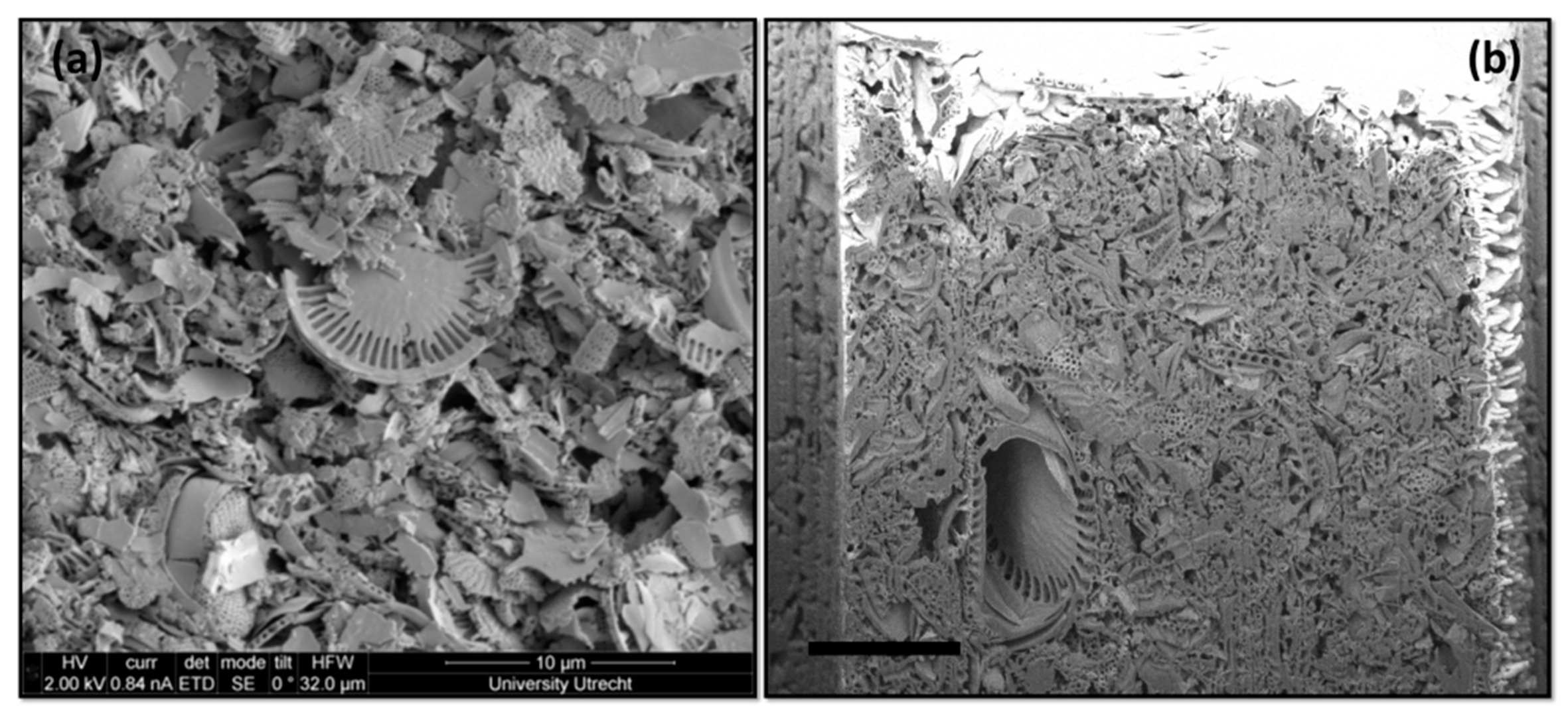
Figure 1. (a) SEM image revealing the surface of the diatomite sample; (b) BSE (backscattered electrons) image of cross section from serial sectioning process, scale bar is 5 µm. The saturated contrast concerns the in situ Pt deposition in BSE imaging.
Minerals 06 00104 g001
Figure 2. SEM images of (a) reacted dunite (olivine-dominated rock) showing the produced amorphous (am) silica rim and (b) the interfacial region between olivine and amorphous silica.
Minerals 06 00104 g002
Figure 3. (a) FIB-SEM of FEI Nova NanoLab 600 (FEI Company, Hillsboro, OR, USA) at Utrecht University; (b) its sample stage (marked by red rectangle) and (c) its inner chamber; (d) the FEI Helios NanoLab G3 UC (FEI Company) at Utrecht University.
Minerals 06 00104 g003
Figure 4. (a) A flow chart showing the serial sectioning procedure of FIB nano-tomography; (b) a schematic indication of one prepared region of interest for tomography technique in a FIB-SEM.
Minerals 06 00104 g004
Figure 5. (a) SE imaging and (b) BSE imaging at 2 kV of the same section in the reacted olivine sample. In the rectangle is a region with curtaining effects; arrows indicate charging effect.
Minerals 06 00104 g005
Figure 6. Trajectories of electrons into a silica-based material, diatomite, simulated by the Monte Carlo method in the Casino software (http://www.gel.usherbrooke.ca/casino/index.html) [66]. Acceleration voltage of the electron beam is 2 kV, incident angle is 38°, and dose is 105. Blue tracks represent incident electrons, whereas red tracks represent backscattered electrons.
Minerals 06 00104 g006
Figure 7. General steps of image processing on tomographic data from serial sectioning procedure.
Minerals 06 00104 g007
Figure 8. (a) Single slice image extracted from the corrected stack generated from the olivine sample; (b) pores are delimited at red outline; (c) result from segmentation of the single slice. The surface area of this slice is about 437 µm2.
Minerals 06 00104 g008
Figure 9. (a) A small region cropped from one slice image showing a big diatom with large pore space that extends in depth (along the Z direction); (b) the watershed segmentation result of this small slice image; (c) a thresholding plus manual correction result of the same region. Two different strategies for segmenting the pore space in the diatomite sample using Avizo: (d) watershed segmentation; (e) thresholding plus manual correction.
Minerals 06 00104 g009aMinerals 06 00104 g009b
Figure 10. 3D rendering of the pores in the explored volume of 23 × 19 × 15 µm3 from the reacted olivine sample, shown in four different orientations. The scale bar is 5 µm.
Minerals 06 00104 g010
Figure 11. Pore size distribution in the obtained volume from the olivine sample. (a) Labelled pores painted in different colours; (b) probability density function of labelled pores size distribution.
Minerals 06 00104 g011
Table 1. Imaging conditions for the serial sectioning performed on porous diatomite and silica materials demonstrated in the present work.
Instrument ConditionsDiatomiteSilica
Electron imaging--
Acceleration voltage (kV)22
Beam current (nA)0.840.84
Imaging typeBSEBSE
DetectorTLDTLD
Resolution image XY (pixels)2048 × 17682048 × 1768
Resolution pixel XY (nm) 12.512.5
Ion milling--
Acceleration voltage (kV)3030
Beam current (nA)0.30.5
Slice thickness (nm)2015
Total number of slices376971

