Numerical Simulations of Two-Phase Flow in a Dorr-Oliver Flotation Cell Model

Abstract

Two-phase (water and air) flow in the forced-air mechanically-stirred Dorr-Oliver machine has been investigated using computational fluid dynamics (CFD). A 6 m³ model is considered. The flow is modeled by the Euler-Euler approach, and transport equations are solved using software ANSYS-CFX5. Unsteady simulations are conducted in a 180-degree sector with periodic boundary conditions. Air is injected into the rotor at the rate of 2.63 m³/min, and a uniform bubble diameter is specified. The effects of bubble diameter on velocity field and air volume fraction are determined by conducting simulations for three diameters of 0.5, 1.0, and 2.0 mm. Air volume fraction contours, velocity profiles, and turbulent kinetic energy profiles in different parts of the machine are presented and discussed. Results have been compared to experimental data, and good agreement is obtained for the mean velocity and turbulent kinetic energy profiles in the rotor-stator gap and in the jet region outside stator blades.

1. Introduction

The hydrodynamics of froth flotation machines controls the grade and rate of recovery achievable in such machines. The complexity of three phase turbulent flow prevalent in those machines defies intuition, and a more scientific approach is needed to understand and control the multiplicity of physicochemical processes responsible for froth flotation. Computational fluid dynamics (CFD) is a powerful methodology that can provide detailed flow field properties such as mean velocity, turbulence intensity, dissipation rate, spatial distribution of air volume fraction (void fraction), bubble size distribution, and bubble-particle collision rate. All of these properties are needed to build simulation models that can be used to predict the grade and rate of recovery. They also help the designer to understand the flow patterns and their impact on flotation processes and to recommend design changes for performance optimization. Furthermore, CFD can provide unsteady forces and moments for structural components (rotor blades, driving shaft, and stator/disperser) needed for assessing structural integrity (stress analysis and vibration), longevity of the machine, and power consumption. Ultimately, CFD is a viable tool to assess the performance of existing flotation cells and to help design the new generation of machines. In the past three years, the authors have used CFD and simulated single and two-phase flows in four well known flotation cells of scales varying from laboratory models to full scale machines [1,2,3,4]. Two of the machines are forced-air machines, namely Dorr-Oliver and Xcell. The third machine is WEMCO cell, which is a self-aerated machine.

Numerical simulation of single phase flow has been conducted to study flow field in “Metso Mineral” and “Outokumpu” 0.8 m³ cell [5]. A 3D grid of sizes 1.56 × 10⁶ for “Metso Mineral” and 1.46 × 10⁶ for “Outokumpu” were used to run the simulations. It illustrates an expensive computational cost especially when the flow inside these flotation cells is unsteady. Single phase simulations may be useful in the initial design stages by providing overall flow characteristics, but in reality, the two phase flow is more relevant to be simulated to determine regions of high void fractions and turbulent dissipation rate. For two-phase simulation, another computational cost is now added to the simulations of the single phase, where another set of transport equations for the gas phase needs to be solved. Some approaches have been used to reduce computational cost [6], where sector-based simulations were used to reduce the number of grid nodes. These simulations provide spatial distribution of turbulent parameters such as turbulent kinetic energy and its rate of dissipation, which are important to identify regions where particles-bubbles attachment and detachment occur [7,8,9,10]. One of the most important parameters in these simulations is the bubble size, which affects directly local void fraction and overall gas hold up in the cell. In real situations, there is no single bubble size but there is a size distribution, which is affected by the local shear and turbulence parameters. In CFD simulation another set of equations that describe particle size distribution “population balance model” can be implemented to predict the bubble size distribution [11]. Of course, it will increase the computational cost because each size group will have its own set of equations. Another approach can be applied to avoid that much computational cost, where a parametric study can be conducted for different bubble size to investigate the effect of the bubble size on the flotation rate.

One of the main functions of mechanical flotation machines is to disperse air bubbles throughout the pulp volume. In order to assess the performance of flotation machines, it is important to know the spatial distribution of dispersed bubbles within the tank volume, which directly affects gas holdup. The current CFD simulations is a parametric study of two-phase flow to provide the hydrodynamic data and air volume fraction spatial distribution for a pre-determined bubble size in the pulp phase in a Dorr-Oliver 6 m³ flotation cell. The results are presented first for a bubble size of 0.5 mm simulation then another two bubble sizes 1.0 and 2.0 mm are used to investigate the effects of the bubble size on the mean flow, turbulent kinetic energy and air volume fraction. Comparisons with experimental data for single and two phase flow are also presented to show that the unsteady Reynolds-Averaged Navier Stokes (RANS) model used in these simulations gives reliable results.

1.1. Euler-Euler Two-Fluid Model

Computational approaches for two phase flow may be classified largely into direct numerical simulation (DNS), Euler-Lagrange, and Euler-Euler models. In the DNS approach [12,13], Navier-Stokes equations are solved for the local velocity and pressure for each phase. This approach is not practical for flotation machines simulations because of the large number of bubbles and high turbulent Reynolds number of the continuous phase. The Euler-Lagrange approach aims at modeling the carrier liquid phase by solving the Reynolds averaged Navier-Stokes equations and tracking bubbles by solving the equations of motion of each bubble as a point mass. Again, this approach is not practical essentially because of the large number of bubbles. The more practical approach is the Euler-Euler approach in which both phases are modeled by volume averaged equations [12]. The motion of the two continuous phases is described by its own RANS equations as the following:

Continuity equation:

(1)

Momentum equation:

(2)

where (i = 1) denotes water phase and (i = 2) denotes gas phase, ∇P is the modified pressure to include the gravity effects, S_i describes any external momentum source (S_i = 0) and M_i is the interfacial force on phase (i) due to the presence of other phases. Momentum exchange between the two phases due to drag and buoyancy on bubbles are the only mechanisms that couple the motion of the two phases. Bubbles are deformable fluid particles when moving in high shear rate regions such as in minerals flotation machines. Schiller-Naumann drag model [14] is used to predict the bubble drag coefficient. Schiller-Naumann drag model [14] neglects the effects of bubble deformation on drag coefficient. Turbulence transport is modeled by the shear stress transport (SST) turbulence model. A universal turbulence model for two-phase flow, particularly at high volume fraction, does not exist [13]. Perhaps the Reynolds stress model is the most adequate model for swirling flows, but it is computationally too demanding, and to the best of our knowledge, has never been applied to two-phase flow in flotation machines.

2. Computational Mesh and Boundary Conditions

The Dorr-Oliver machine is a mechanically agitated flotation cell. Two-phase (water and air) simulations are conducted for a 6 m³ model of the machine. The overall dimensions of the model are shown in Figure 1. The machine is equipped with a 6-blade rotor surrounded by a 16-blade stator. Air is injected continuously into the rotor through six slots on the hub of the six passages of the rotor. Simulations are conducted for rotor speed of 250 rpm (N = 4.167 rev/s), maximum rotor diameter of 0.49 m, Reynolds number (ND²/ν) of 1.0 × 10⁶, and air volume rate (Q) 2.633 m³/min. These conditions give rotor tip speed (U) of 6.414 m/s and average inlet air speed of 7.0 m/s. To investigate the effects of bubble diameter on gas hold up and other flow properties, separate simulations are performed for bubble diameters (D_b) of 0.5, 1.0, and 2.0 mm. The flow in a 180-degree sector is simulated by applying periodic boundary conditions. This choice of computational domain is dictated by the number of rotor blades of which there are six, and the number of stator blades of which there are 16. Therefore, the smallest circumferential sector that allows periodic boundary conditions must include three rotor blades and eight stator blades; that is half the machine.

A block-structured mesh is generated on half the machine using 1.2 million nodes. The mesh in a vertical plane through the central axis is shown in Figure 2a, and a close-up of the surface mesh on the rotor and stator blades is shown in Figure 2b. Geometric details of the rotor and stator are very precisely represented by the geometric model. Fine grids are used near solid walls, particularly the leading edges of rotor blades in order to resolve tip vortices and high suction regions. The rotor is embedded in a rotating volume whose surface is a body of revolution. The impeller rotation is modeled by the Rotating Frame of Reference (RFR) approach because it correctly represents the unsteady interaction between the rotor and stator blades. The commonly used Multiple Frames of Reference (MFR) approach is inaccurate because the stator-rotor interaction is treated by the Frozen Rotor frame change model. All equations are advanced in time by using first-order implicit Euler method. The unsteady calculations have been performed on 8 parallel processors. The time step (∆t) is equal to 0.002 s, and at 250 rpm, the impeller volume rotates (∆θ) equal to 3.0 degrees per time step. Five sub-iterations are used per time step, and the residual RMS of each equation was less than 5 × 10⁻⁴ at the end of each time step.

Figure 1. Overall dimensions of a 6 m³ model of Dorr-Oliver flotation cell.

Figure 1. Overall dimensions of a 6 m³ model of Dorr-Oliver flotation cell.

Figure 2. (a) Block structured mesh and (b) surface grids on rotor and stator blades.

Figure 2. (a) Block structured mesh and (b) surface grids on rotor and stator blades.

No-slip boundary condition is imposed on all solid walls. The flow in a small duct leading to the air injection opening is modeled, and inlet boundary condition with specified air normal-velocity is specified on the inlet to the duct. The top surface of the actual tank is extended into an overflow tank (not shown in figures). Outflow boundary condition with prescribed air velocity that satisfies global conservation of air volume flow rate through the machine is imposed at the top of the overflow tank. This treatment of the tank top boundary condition is more suitable for unsteady flow than the degassing boundary condition. This is because air holdup and pulp interface are not known a priori. The actual tank is initialized with 100% water, and the overflow tank is initialized with 100% air. The overflow tank is used to permit the water level to rise due to the accumulation of air in the pulp, and at the same time, it does not allow water to exit the computational domain. No boundary conditions are needed at the interface between the actual tank and the overflow tank. The governing equations of the two-phase flow are solved in both tanks allowing air and water to flow between the tanks as required by the transport equations.

3. Results and Discussion

3.1. Flow Details for D_b = 0.5 mm

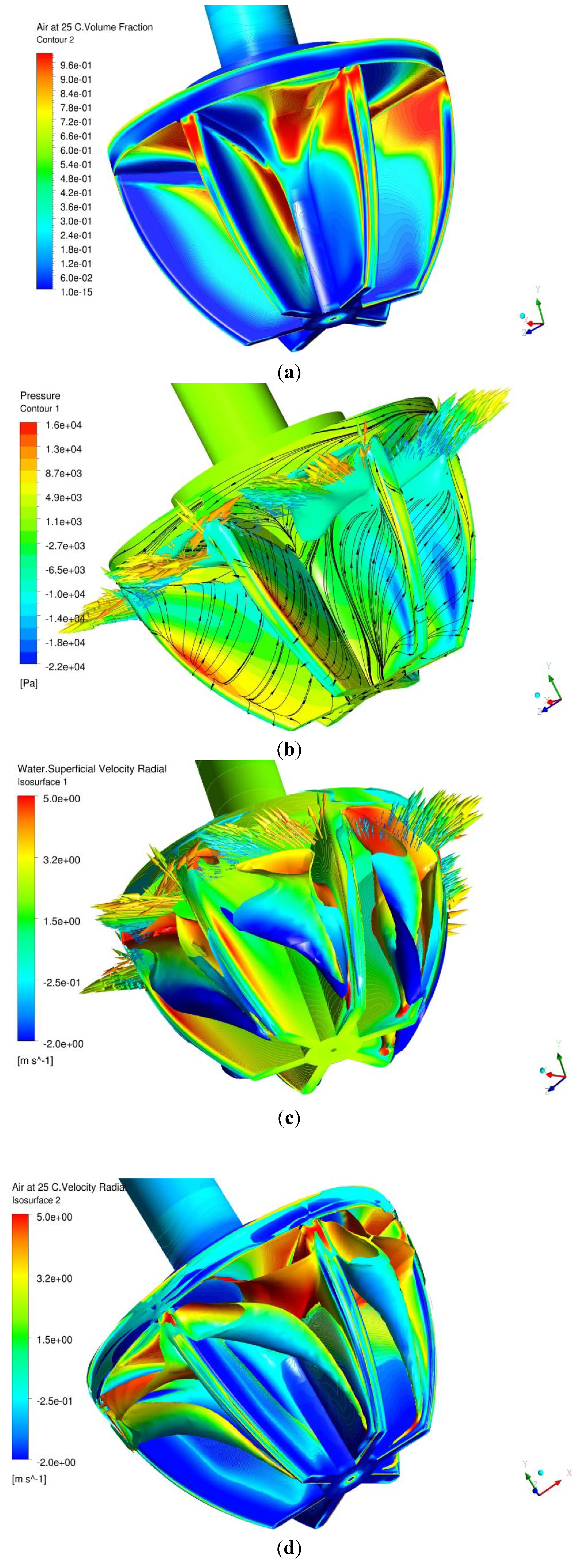
The results for the case of bubble diameter of 0.5 mm will be presented in more details here. The effects of bubble diameter will be briefly discussed. Contours of air volume fraction (α) on the rotor surface are depicted in Figure 3a. Upon exiting the injection slots, air adheres to the rotor top plate and drifts towards the suction sides (these are the receding faces) of the rotor blades. Air exits the rotor mainly from corners at the intersections of the suction sides of the blade with the ceiling of rotor. The major part of pressure sides (advancing surfaces) is wetted with water. Shown in Figure 3b are pressure (P) contours (flooded contours) and friction lines (black lines) that give the direction of water velocity (relative to the rotor) very close to the rotor surface. Friction lines show attachment line in the region of high pressure near the leading edges of the blades.

Water flows inward on the pressure sides and outward on the suction sides, which implies the presence of passage vortices. Relative superficial air velocity vectors at the rotor exit are concentrated near the rotor top and mainly near the suction sides. These vectors are colored by the local air volume fraction. Also shown in the figure is an iso-surface of air volume fraction equal to (α = 0.6). Iso-surface of water relative velocity magnitude (V_wr) of 5.0 m/s is shown in Figure 3c. The iso-surface is colored by the water radial velocity component. The negative radial velocity (blue color) indicates that water enters rotor passages through the lower two thirds of rotor and exits through the upper one third with maximum outward radial velocity near the end plate. Also shown in the figure are air relative velocity vectors, which are colored by the air volume fraction. An air jet exits the rotor passage near the upper corner, above and somewhat segregated from the water jet. An iso-surface of air volume fraction of (α = 0.1) is used to show the passage vortices, which are shown in Figure 3d. The iso-surface is colored by air radial velocity. The blue color on bottom (negative radial velocity) and the red color on top (positive radial velocity) clearly indicate the presence of a vortex.

The vortex is floated on the suction side of the blade and exits the rotor near the upper corner of the pressure side. The vortex is made visible by air bubbles trapped in the vortex core. In addition, as air is injected into the rotor it is squeezed by the water flow towards the rotor end wall.

Figure 3. (a) Air volume fraction (α) on rotor surface; (b) pressure (P) contours on rotor surface; (c) iso-surface of water superficial relative velocity (V_wr = 5.0 m/s); and (d) iso-surface of air volume fraction (α = 0.1) showing rotor passage vortices.

Figure 3. (a) Air volume fraction (α) on rotor surface; (b) pressure (P) contours on rotor surface; (c) iso-surface of water superficial relative velocity (V_wr = 5.0 m/s); and (d) iso-surface of air volume fraction (α = 0.1) showing rotor passage vortices.

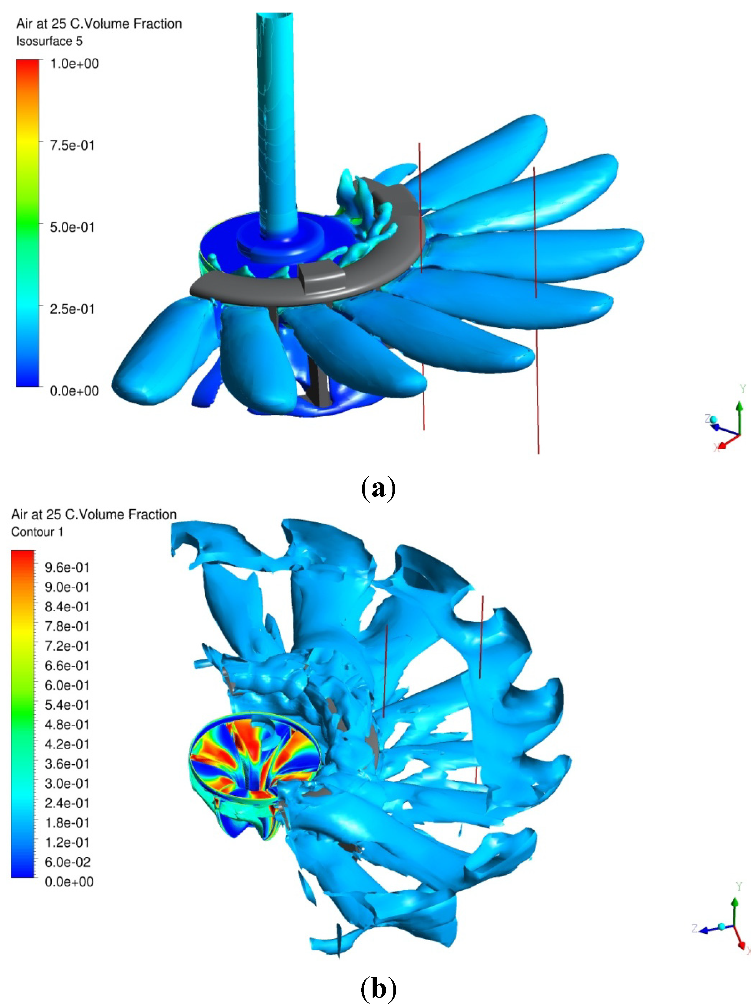
Next, we discuss the flow characteristics downstream of the stator blades. The flow exits the upper third of the rotor as six pulsating jets with strong radial and circumferential velocity components. The six jets impinge on the sixteen-blade stator and emerge from the stator as sixteen radial jets. The jet locations relative to stator are shown in Figure 4a by water superficial velocity (V_w) iso-surface of 0.92 m/s, which is colored by air volume fraction. As the flow exits the rotor and impinges on stator blades leading edges, a small fraction of it splashes over the ring carrying some of the high air volume fraction above the ring as indicated by the color of the small eight tongs between rotor and stator. The major part of flow, however, goes below the stator ring.

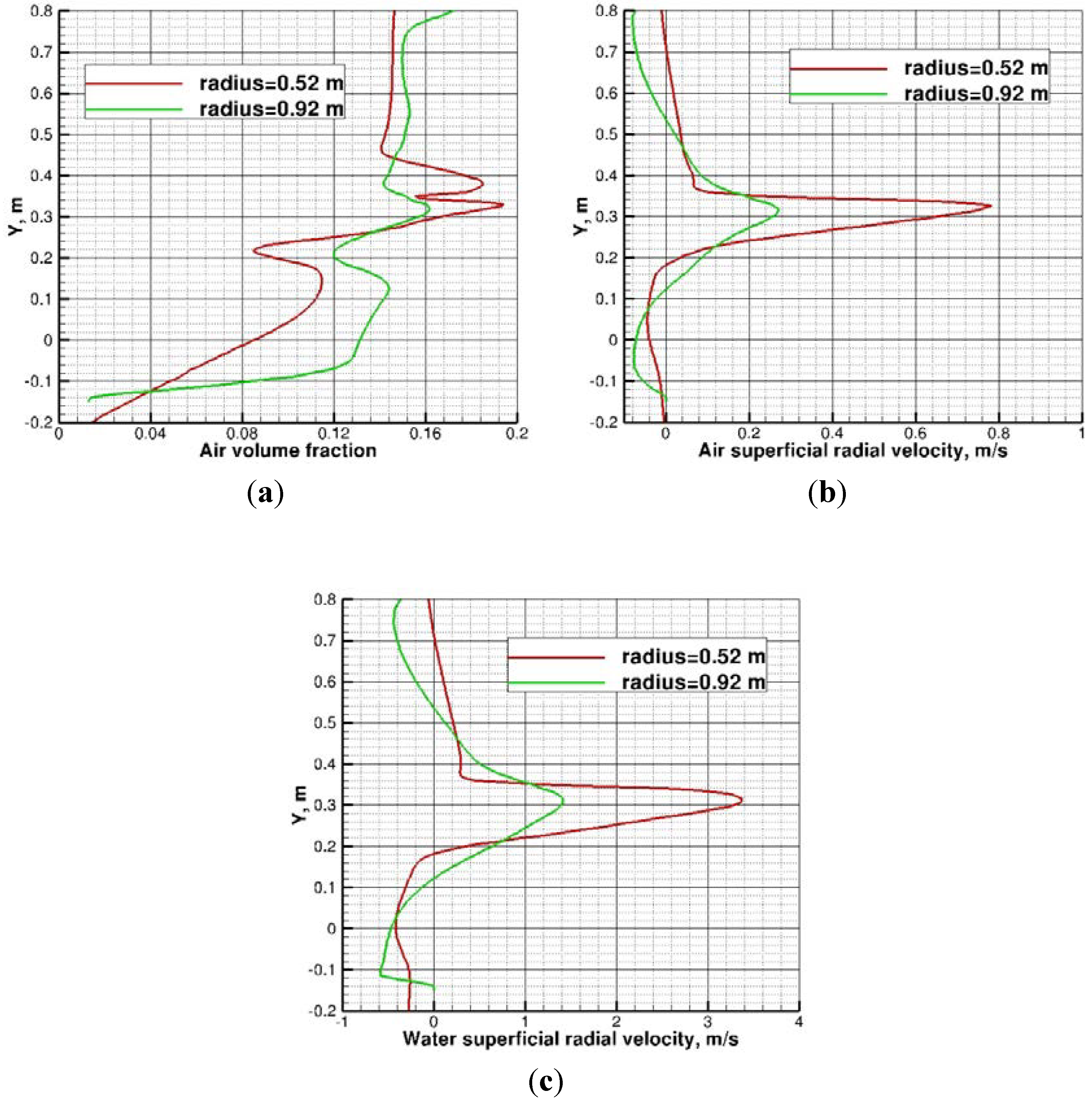
Figure 4b shows an iso-surface of air volume fraction of (α = 0.15) and the contours of air volume fraction on the rotor surface. Air bubbles are mainly convected by the jets towards the tank walls. Some of the air-rich flow splashes on the stator blades and escapes through the gap between rotor and stator. Air volume fraction, air superficial radial velocity, and water superficial radial velocity profiles on two vertical lines at radial distances (r = 0.52 and 0.92 m) are shown Figure 5a–c, respectively. Air volume fraction profiles very close to the stator at r = 0.52 m shows a double peak, but only the lower peak is convected as can be deduced from the air superficial radial velocity profile shown in Figure 5b. The air volume fraction profile at r = 0.92 m shows a maximum in the jet region but also an increase in air concentration above and below the jets. As the jets impinge nearly normally on the tank walls, they recirculate part of the air into the lower and upper portions of the tank. The velocity profiles diffuse due to turbulent momentum transport and also because of the increase of flow area in the radial direction. Negative radial velocity indicates the return flow into the rotor region. The jets are directed slightly upward, and the two profiles for air and water are somewhat similar in the jet regions.

Figure 4. (a) Iso-surface of water superficial velocity (V_w = 0.92 m/s) showing jets downstream of stator and (b) iso-surface of air volume fraction of (α = 0.15), lines at radii r = 0.52 and 0.92 m.

Figure 4. (a) Iso-surface of water superficial velocity (V_w = 0.92 m/s) showing jets downstream of stator and (b) iso-surface of air volume fraction of (α = 0.15), lines at radii r = 0.52 and 0.92 m.

Figure 5. (a) Air volume fraction (α) at r = 0.52 (red) and 0.92 m (green); (b) Air superficial radial velocity (V_a,radial) at r = 0.52 (red) and 0.92 m (green); and (c) Water superficial radial velocity (V_w,radial) at r = 0.52 (red) and 0.92 m (green).

Figure 5. (a) Air volume fraction (α) at r = 0.52 (red) and 0.92 m (green); (b) Air superficial radial velocity (V_a,radial) at r = 0.52 (red) and 0.92 m (green); and (c) Water superficial radial velocity (V_w,radial) at r = 0.52 (red) and 0.92 m (green).

3.2. Effects of Bubble Diameter on Void Fraction

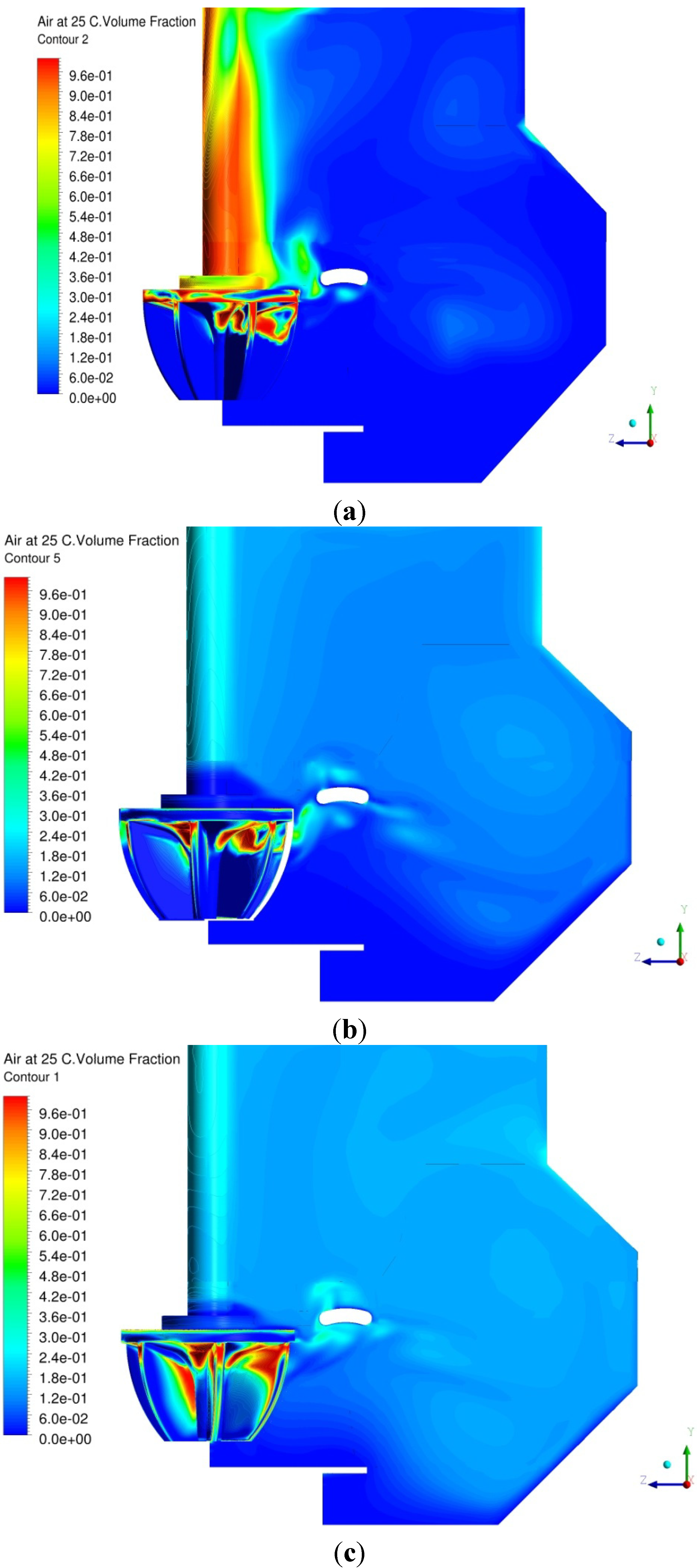
In the present two-phase flow simulations, a uniform bubble diameter is used. To study the effects of bubble diameter on the flow characteristics, three separate simulations for bubble diameters of 2.0, 1.0, and 0.5 mm are conducted. Air volume fraction contours in a vertical plane passing through jet region are shown in Figure 6a–c for the three mentioned bubble diameters, respectively.

As shown in Figure 6a for a large bubble diameter of 2 mm, higher buoyancy force relative to drag causes air bubbles to escape through the gap between rotor and stator. The portion of air that escapes through the gap drifts towards the shaft (low pressure region due to centrifugal forces) and rises upward to the water surface. The portion of air bubbles that passes through stator is convected with water jets and rises upward near tank walls towards water free surface. Most of the air for this bubble diameter escapes through the gap between rotor and stator. Negligible amount of air bubbles are convected downward with water stream to re-enter the rotor.

Similarly, it is concluded from Figure 6b that for bubble diameter of 1 mm, buoyancy force on air bubbles is still high enough to cause some air to escape through the gap between rotor and stator. The portion of air bubbles that passes through stator is convected with water jets and drifts upward near tank walls towards water surface. Some of the air is convected downward into lower portion of the tank. The air is well dispersed throughout the tank.

Unlike the previous two cases, as shown in Figure 6c for a small bubble diameter of 0.5 mm, higher drag relative to buoyancy causes air bubbles to travel longer with water jets. Most of the air bubbles pass through stator and are convected with water stream. Air bubbles are dispersed throughout the tank volume, and some air re-enters the rotor.

Figure 6. (a) Air volume fraction (α) contours for bubble diameter = 2 mm; (b) Air volume fraction (α) contours for bubble diameter = 1 mm; and (c) Air volume fraction (α) contours for bubble diameter = 0.5 mm.

Figure 6. (a) Air volume fraction (α) contours for bubble diameter = 2 mm; (b) Air volume fraction (α) contours for bubble diameter = 1 mm; and (c) Air volume fraction (α) contours for bubble diameter = 0.5 mm.

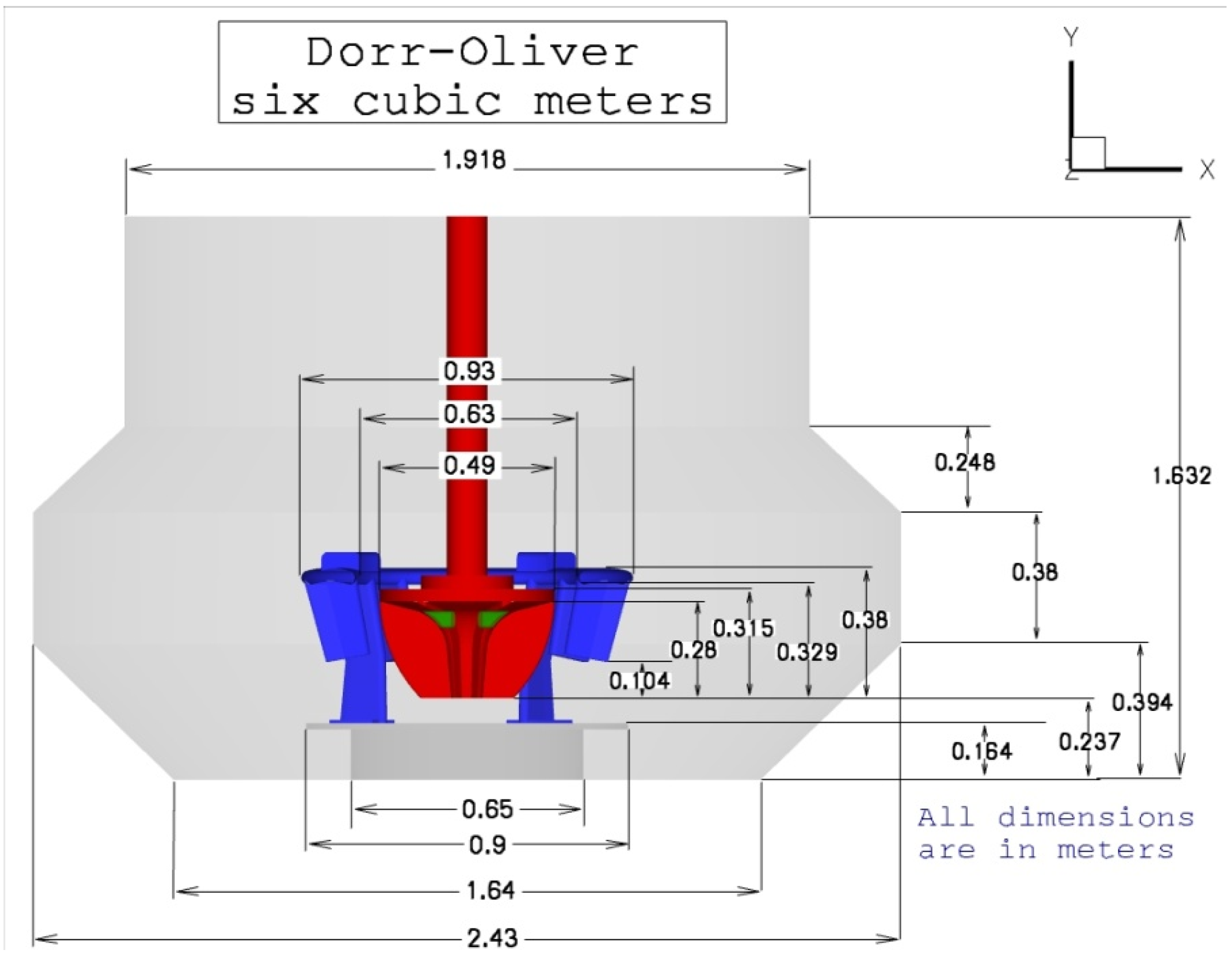
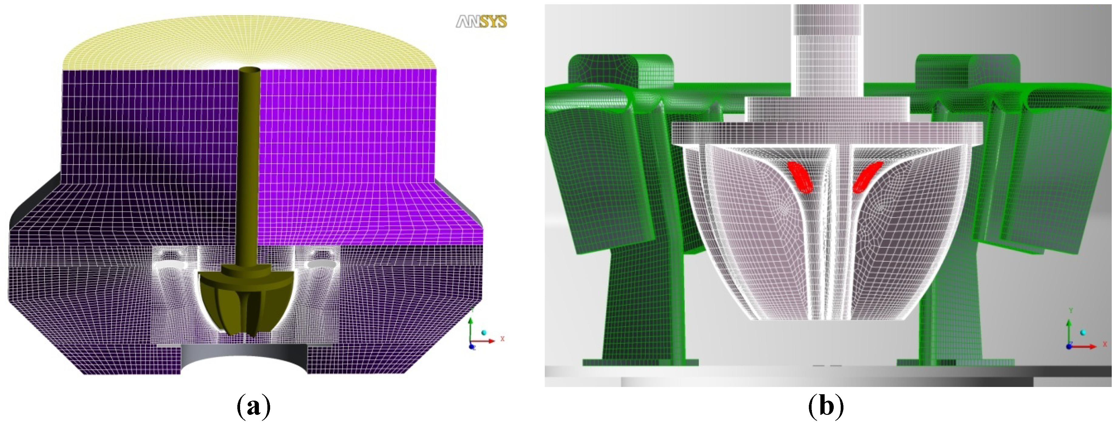
3.3. Comparison of CFD Results with Experiments

Validation of the computational model is very important to build confidence in CFD as a viable tool for the analysis of such a complex two-phase flows. The flow in a flotation cell poses many challenges to both CFD modeling and experimental measuring techniques. Such challenges including three-dimensional unsteady shear flow, turbulence production and dissipation, rotating components, and multiphase phenomena. Mean velocity and turbulence statistics have been measured in a 6 m³ Dorr-Oliver pilot cell for both single and two phase flow [15,16].

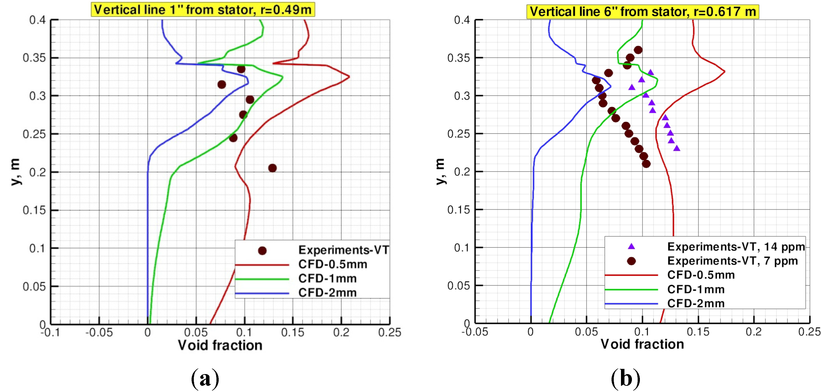
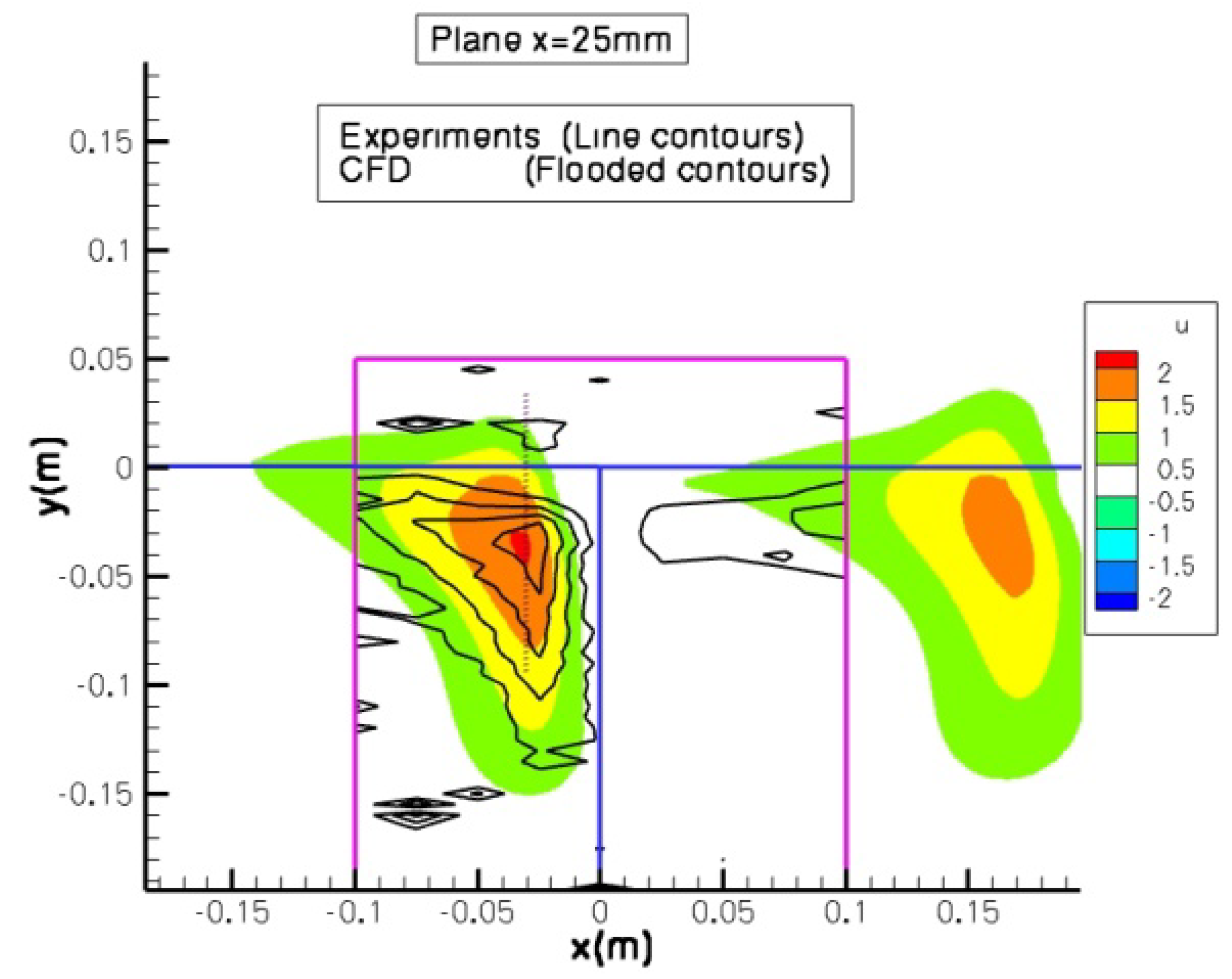
Comparisons between CFD and experimental data [15,16] for void fraction on two vertical lines outside stator are shown in Figure 7a,b. An iso-kinetic probe had been developed and used to measure air void fraction [16]. The comparison in Figure 7a,b shows that the CFD agrees with the experimental data in the jet region for bubble diameter (D_b) of 1.0 mm. Away from the stator, the overall level air volume fraction of CFD is comparable to the level of the experimental data however the trend below the jet is different. This may be attributed to the production of smaller bubbles (smaller than the diameter specified in the simulations) in the jet shear layers thereby increasing the local void fraction as supported by the increase of the void fraction below the jets as the bubble size decreases from 2.0 to 0.5 mm. In the simulation, gas holdup is 13%, 8% and 3% for bubble diameters of 0.5, 1.0 and 2.0 mm, respectively. Experimental gas holdup reports 6.8% where a bubble size distribution exists in the physical experiment.

Figure 7. (a) Air volume fraction (α) profile at 25.4 mm downstream of stator and (b) air volume fraction (α) profile at 152.4 mm downstream of stator.

Figure 7. (a) Air volume fraction (α) profile at 25.4 mm downstream of stator and (b) air volume fraction (α) profile at 152.4 mm downstream of stator.

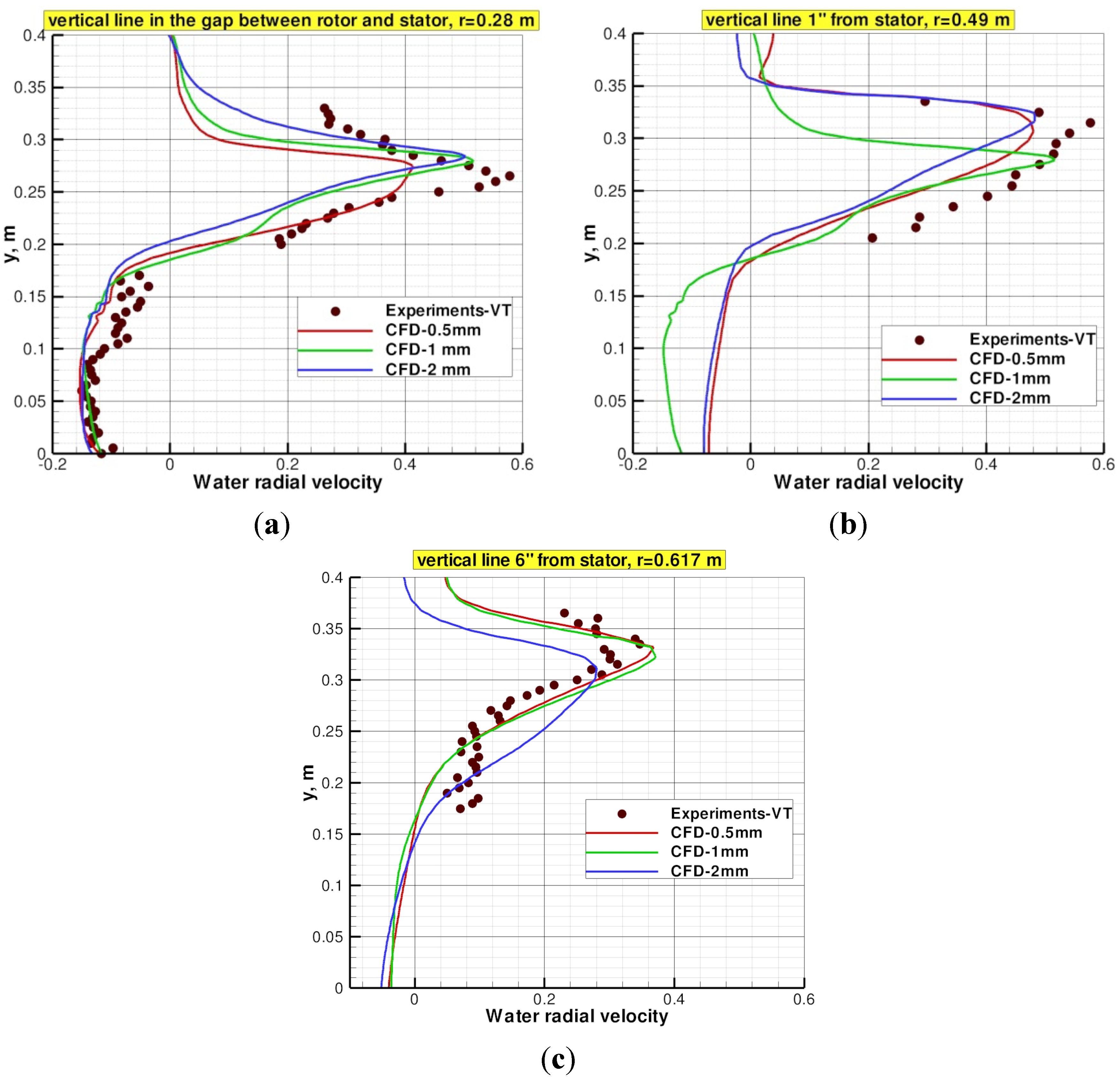
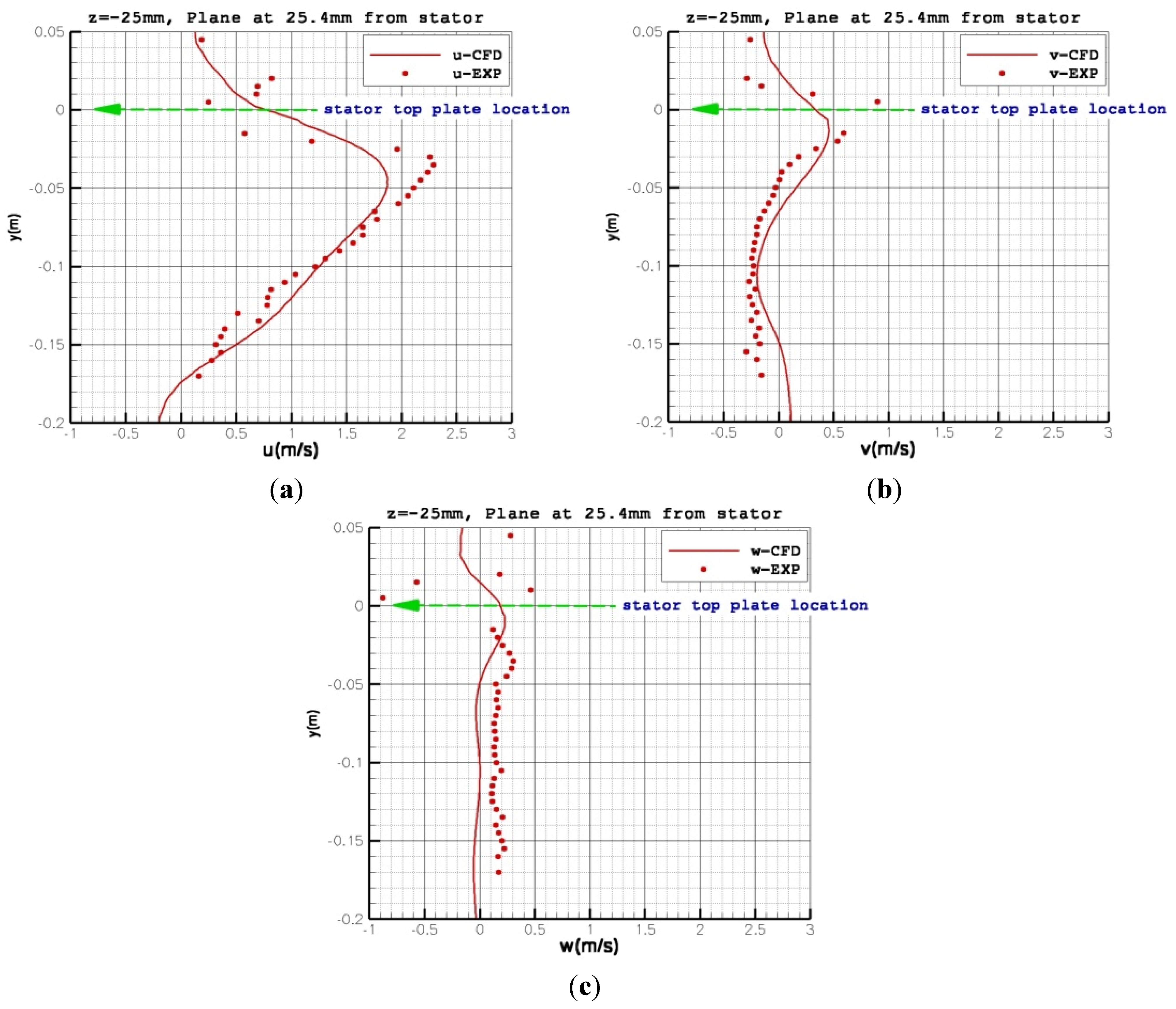
Water superficial velocity profiles on vertical lines in the gap between rotor and stator and outside that region are shown in Figure 8 and Figure 9. All velocities are normalized by the rotor tip speed (U = 6.414 m/s.). Each profile is an average over 16 vertical lines that have the same circumferential location relative to the stator; which has 16 blades; however, they are not averaged over time.

It is evident from Figure 8 that the bubble diameter has some effects on the water superficial radial velocity within and outside the rotor-stator regions. CFD profiles for 1.0 mm bubble diameter show good agreement with the experimental data. Of course, in the experiments, a bubble size distribution exists, and the present simulations suggest that the most probable bubble diameter is 1.0 mm.

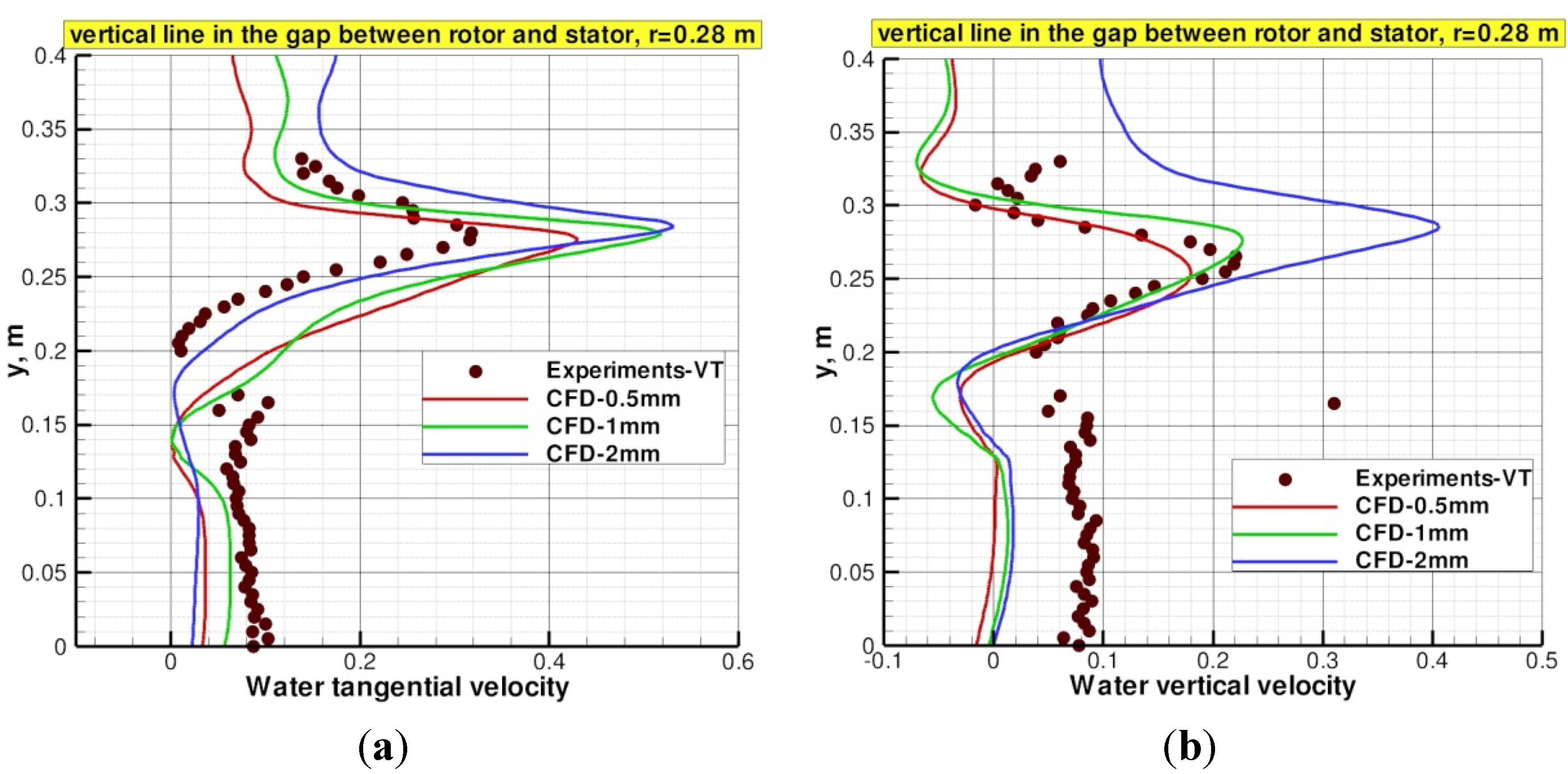
Comparison between CFD profiles and experimental data for tangential and vertical velocity components in the gap between rotor and stator are depicted in Figure 9a,b, respectively. Very good agreement is obtained in that region for bubble diameters of 1 and 0.5 mm. The strong buoyancy effects on the larger bubble diameter of 2 mm gives significantly higher vertical water velocity in the gap. Outside the stator, the tangential component is small in comparison to the radial component; not presented here.

The comparison shows some deviations between experimental and CFD results due to the existence of multi-size bubbles in the experimental work, while in CFD work a mono-size of the bubbles has been applied. Other sources of uncertainty in the CFD model is the model used to evaluate drag on bubbles which is valid only at low volume fraction, whereas in this machines regions of volume fraction as high as 100% exist. Notwithstanding the deviations between CFD and experimental data, and considering the complexity of such a flow, the agreement between CFD results and experimental data is deemed good; which lends strong support for the validity of the CFD model.

Figure 8. (a) Normalized water superficial radial velocity on a vertical line r = 0.28 m in the gap between the rotor and stator; (b) normalized water superficial radial velocity on a vertical line at radial distance 25.4 mm from the stator ring; and (c) normalized water superficial radial velocity on a vertical line at radial distance 152.4 mm from the stator ring.

Figure 8. (a) Normalized water superficial radial velocity on a vertical line r = 0.28 m in the gap between the rotor and stator; (b) normalized water superficial radial velocity on a vertical line at radial distance 25.4 mm from the stator ring; and (c) normalized water superficial radial velocity on a vertical line at radial distance 152.4 mm from the stator ring.

Figure 9. (a) Normalized water superficial tangential velocity on a vertical line r = 0.28 m in the gap between the rotor and the stator and (b) normalized water superficial vertical velocity on a vertical line r = 0.28 m in the gap between the rotor and the stator.

Figure 9. (a) Normalized water superficial tangential velocity on a vertical line r = 0.28 m in the gap between the rotor and the stator and (b) normalized water superficial vertical velocity on a vertical line r = 0.28 m in the gap between the rotor and the stator.

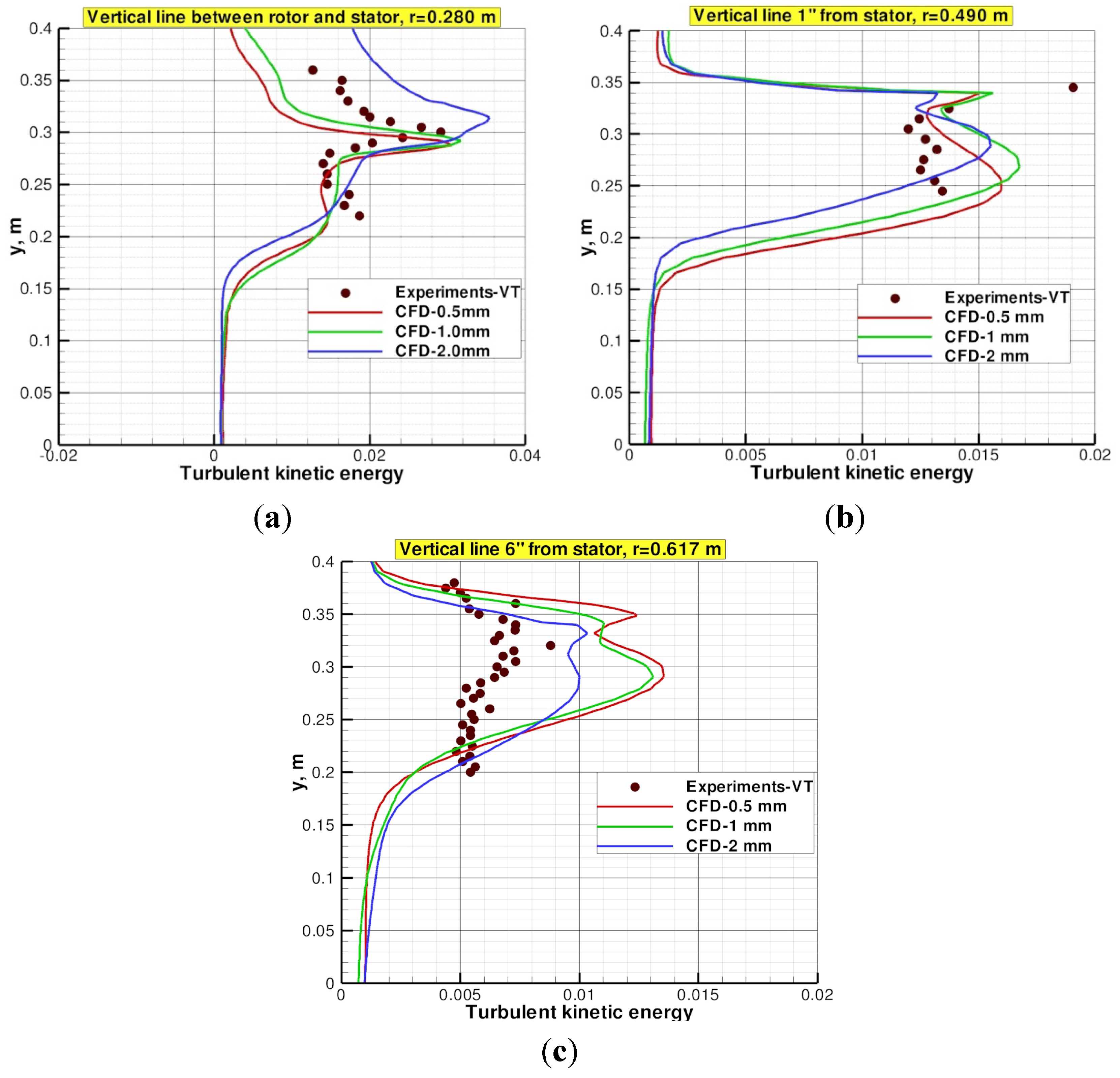
Figure 10 shows a comparison between CFD and experiments [15,16] for turbulent kinetic energy (TKE) normalized by the square of the rotor tip speed (U²) in different regions in Dorr-Oliver 6 m³ pilot cell. High levels of turbulent kinetic energy are predicted in the gap between rotor and stator. The high levels are localized in the high speed jets out of the rotor. As the jets impinge on stator blades, they break up into smaller jets downstream of the stator resulting in a more uniform distribution of turbulent kinetic energy but over a larger volume. Very good agreement is obtained for bubble diameter (D_b) of 1.0 mm in the gap between rotor and stator. In addition, good agreement is obtained immediately downstream of the stator, but there is significant differences in the region far from the stator. As mentioned earlier the bubble size distribution in the experiments could cause these deviations, and also the turbulence model utilized with the RANS equations in the CFD model does not account for bubble induced turbulence, its importance is noted by Van den Akker [13]. Generally, turbulence in the continuous phase may be generated by shear due to large-scale velocity gradient as well as by the presence and relative motion of the dispersed phase. In addition, the dispersed phase may exhibit a turbulent flow behavior in response to the turbulent motions of the continuous phase. Another source of uncertainties in the CFD results is the fact that in unsteady RANS simulations there is no clear-cut distinction between time scales, some scales are treated by the turbulence models, and others are resolved by the averaged equations. There are also uncertainties in the experimental data. The CFD results are encouraging; however, further improvements in turbulence modeling for multiphase flow are needed. Further validation for single phase flow is presented in the appendix.

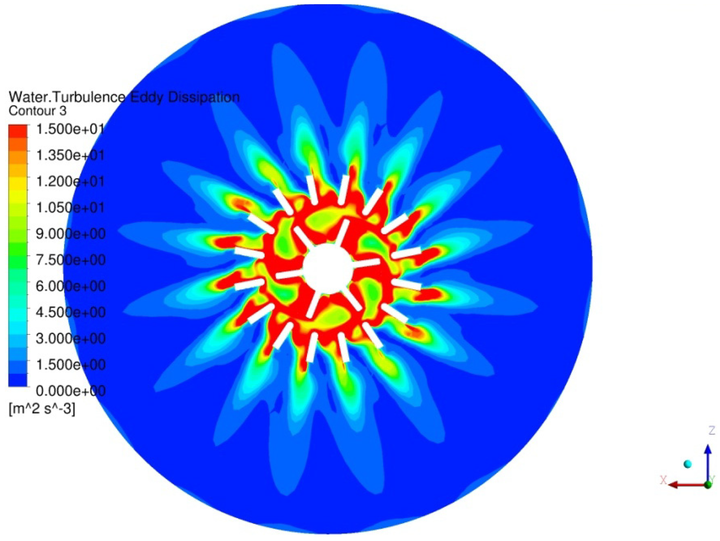
Figure 11 shows contours of the turbulent kinetic energy dissipation rate (ε) in a horizontal plane passing through the rotor, stator and the tank at the jets maximum velocity. TKE dissipation rate are maximum in the regions between rotor and stator and between stator blades. Ragab and Fayed [3] showed that high dissipation rate has favorable effects on collisions frequency of particles and bubbles in the regions between rotor and stator blades. Nevertheless, high dissipation rate has also adverse effects on the attachment probability in these regions.

Figure 10. (a) Normalized TKE on a vertical line r = 0.28 m in the gap between the rotor and the stator; (b) normalized TKE along vertical line at 25.5 mm from the stator ring in the radial direction; and (c) normalized TKE on a vertical line 152.4 mm from the stator ring in the radial direction.

Figure 10. (a) Normalized TKE on a vertical line r = 0.28 m in the gap between the rotor and the stator; (b) normalized TKE along vertical line at 25.5 mm from the stator ring in the radial direction; and (c) normalized TKE on a vertical line 152.4 mm from the stator ring in the radial direction.

Figure 11. Turbulent kinetic energy dissipation rate in a horizontal plane passing through the jets.

Figure 11. Turbulent kinetic energy dissipation rate in a horizontal plane passing through the jets.

4. Conclusions

In this paper, two-phase (water and air) flow in a 6 m³ model of Dorr-Oliver flotation cell, which is an air-forced mechanically-stirred machine, is simulated. Euler-Euler two-fluid approach is used, and the transport equations are solved in time (unsteady simulation). A block structured grid is used to model a 180-degree sector (half the machine) and rotationally periodic boundary conditions are enforced. Air flow rate is specified, and uniform bubble diameter is assumed. A novel treatment of the free surface boundary condition is introduced. The results indicate:

(a)

Air injected into the rotor is squeezed between the rotor solid surface and the water pumped by the rotor. The air-water flow exits the upper one-third of the rotor passage with air-rich above water-rich flow. The air-rich flow drifts towards the suction (or receding) sides of the rotor blades, while the water-rich flow drifts towards the pressure (or advancing) sides of the rotor blades. Thus, air is not fully dispersed at the rotor exit, but is somewhat segregated from water.

(b)

For large bubble diameter (D_b = 2 mm), higher buoyancy relative to drag causes most of the injected air to escape through the gap between rotor and stator.

(c)

For small bubble diameter (D_b = 0.5 mm), higher drag relative to buoyancy causes air bubbles to travel longer distances with water jets. Most of the air bubbles pass through stator and is convected with the water stream. Some air re-circulates in the bottom tank, re-enters the rotor and accumulates in the core of rotor passage vortices, which are low pressure regions.

(d)

Bubble diameter has significant effects on the gas hold up. Higher gas hold up ratio is observed for smaller bubble diameters.

(e)

High levels of turbulent kinetic energy are predicted in six (number of rotor blades) regions between rotor and stator. These regions, however, are localized in the high speed jets out of the rotor. As these jets impinge on stator blades, they breakup into 16 (number of stator blades) smaller jets downstream of stator resulting in a more uniform distribution of turbulent kinetic energy over a larger volume.

(f)

Flow exits stator as spinning radial jets (16 jets) that impinge on tank wall forming strong recirculation region in the lower part of the tank, and a weaker circulation in the upper part.

CFD results have been validated by comparison with experimental data [15,16]. The comparisons show:

• Good to fair agreement between CFD and experimental data for the mean velocity profiles at different radial locations. The results indicate that the most probable bubble diameter is around 1.0 mm.
• CFD predicts correct trend and profiles of TKE.
• In addition, for single phase (water) simulations, good agreement for pressure distribution on stator windward sides is obtained. CFD predicts the right trend for pressure distribution on leeward side of stator blades but fair agreement for pressure magnitude.

This work demonstrates the viability and validity of CFD as a technique that can provide detailed description of the two-phase flow in a flotation cell. Further developments of the computational model, however, are still needed. In view of the important effects of bubble diameter on two-phase simulations, future simulations should account for a distribution over a range of bubble diameter. The effects of bubble breakup and coalescence using a population balance model should also be considered. More simulations are needed to determine sensitivity of CFD results to drag coefficient and turbulence models. Existing bubble drag models assume very low void fraction; drag models that account for high volume fraction need to be developed. The complex three-dimensional unsteady shear flow calls for a more detailed description of the important large scales of turbulence. It is feasible to apply large-eddy simulations to predict multiphase flow in flotation machines.

References

1. Salem-Said, A.; Fayed, H.; Ragab, S. CFD Simulation of a Dorr-Oliver Flotation Cell. In Proceedings of the SME Annual Meeting and Exhibit, Denver, CO, USA, 28 February–2 March 2011.
2. Fayed, H.; Ragab, S. CFD Analysis of Two-Phase Flow in a Self Aerated Flotation Machine. In Proceedings of the SME Annual Meeting and Exhibit, Seattle, WA, USA, 19–22 February 2012.
3. Ragab, S.; Fayed, H. CFD-Based Flotation Model for Prediction of Pulp Recovery Rate. In Proceedings of the SME Annual Meeting and Exhibit, Seattle, WA, USA, 19–22 February 2012.
4. Fayed, H.; Ragab, S. CFD Analysis of Two-Phase Flow in WEMCO 300 m3 Supercell. In Proceedings of the SME Annual Meeting and Exhibit, Denver, CO, USA, 24–27 February 2013.
5. Koh, P.T.L.; Schwarz, P.; Zhu, Y.; Bourke, P. Development of CFD Models of Mineral Flotation Cells. In Proceedings of the 3rd International Conference on CFD in the Minerals and Process Industries, Melborne, Australia, 10–12 December 2003; pp. 171–175.
6. Tiitinen, J.; Koskinen, K.; Ronkainen, S. Numerical Modeling of an Outokumpu Flotation Cell. In Proceedings of the Centenary of Flotation Symposium, Brisbane, Australia, 6–9 June 2005.
7. Koh, P.T.L.; Schwarz, M.P. CFD modeling of bubble-particle attachments in flotation cells. Miner. Eng. 2006, 19, 619–626. [Google Scholar] [CrossRef]
8. Koh, P.T.L.; Schwarz, M.P. CFD model of a self-aerating flotation cell. Int. J. Miner. Process. 2007, 85, 16–24. [Google Scholar] [CrossRef]
9. Evans, G.; Doroodchi, E.; Lane, G.; Koh, P.; Schwarz, P. Mixing and Gas Dispersion in Mineral Flotation Cells. In Proceedings of the 6th International Symposium on Mixing Industrial Process Industries (ISMIP VI), Niagara on the Lake, Canada, 17–21 August 2008.
10. Koh, P.T.L.; Schwarz, M.P. Models of Microcell and Jameson Flotation Cells. In Proceedings of the 7th International Conference on CFD in the Minerals and Process Industries, Melbourne, Australia, 9–11 December 2009.
11. Kerdouss, F.; Bannari, A.; Proulx, P. CFD modeling of gas dispersion and bubble size in a double turbine stirred tank. Chem. Eng. Sci. 2006, 61, 3313–3322. [Google Scholar] [CrossRef]
12. Prosperetti, A.; Tryggvason, G. Computational Methods for Multiphase Flow; Cambridge University Press: Cambridge, UK, 2007. [Google Scholar]
13. Van den Akker, H.E.A. Toward a truly multiscale computational strategy for simulating turbulent two-phase flow processes. Ind. Eng. Chem. Res. 2010, 49, 10780–10797. [Google Scholar] [CrossRef]
14. Clift, R.; Grace, J.R.; Weber, M.E. Bubbles, Drops and Particles; Dover Publications: Mineola, NY, USA, 2005. [Google Scholar]
15. Yang, Y.; Telionis, D. Turbulence Measurements in a Flotation Cell Using Fast-Response Probe. In Proceedings of the 2011 SME Annual Meeting, Denver, CO, USA, 28 February–2 March 2011.
16. Yang, Y. Experimental Study of Multi-Phase Flow Hydrodynamics in Stirring Tanks. Ph.D. Thesis, Virginia Tech, Blacksburg, VA, USA, 4 February 2011. [Google Scholar]