Particle Swarm Optimization (PSO) of High-Quality Magnetic Data of the Obudu Basement Complex, Nigeria

Abstract

The particle swamp optimization procedure was applied to high-quality magnetic data acquired from the Precambrian Obudu basement complex in Nigeria with the object of estimating the distinctive body parameters (depth (z), index angle (θ), amplitude coefficient (K), shape factor (Sf), and location of the origin (x₀)) of magnetic models. The magnetic models were obtained from four profiles that ran perpendicular to the observed magnetic anomalies within the study area. Profile A–A’ with a length of 2600 m is characterized by inverted model parameters of K = 315.67 nT, z = 425.34 m, θ = 43°, Sf = 1.15, and x₀ = 1554.86 m, while profile B–B’ with a length of 5600 m is described by K = 257.71 nT, z = 543.75 m, θ = 54°, Sf = 0.96, and x₀ = 3645.42 m model parameters. Similarly, profile C–C’ with a length of 3000 m is defined by K = 189.53 nT, z = 560.87 m, θ = 48, Sf = 1.2, and x₀ = 1950 m. Profile D–D’, which is well-defined by a 2500 m length, started at the crest of the observed magnetic anomaly and displays inverted model parameters of 247.23 nT, 394.16 m, 39°, 1.26, and 165.41 m. Correlatively, the estimated shape factor of the four models (Sf = 1.15, 0.96, 1.2, and 1.26) shows that the magnetic models are linked to thin sheets. Furthermore, quantitative interpretations of the models show that the PSO operation is rapid and proficient.

1. Introduction

High-resolution magnetic data analysis has been applied extensively to mineral and ore explorations worldwide [1,2,3]. Additionally, it can be used in the investigation of hydrocarbon [4], engineering surveys [5,6], detection of UXO [2], mapping of geothermal anomalies [7,8], archaeological investigations [9], and delineation of subsurface hydrological structures [3,5]. Moreover, almost all magnetic data analysis procedures are performed believing that the subsurface features are simple geometrical structures, such as thin sheets, horizontal cylinders, spheres, and faults (caused by diverse ore and mineral-bearing bodies, as well as structural hydrocarbon traps), which are buried at various depths [5,10].

A number of inversion procedures are used in general to evaluate parameters connected with simple geologic models, such as geologic contacts, cylinders, spheres, and thin sheets [11,12,13]. In several tasks, these models assume notable roles [13]. However, while it may be challenging to precisely define the geological origins of these models resulting from subsurface magnetic bodies, they still hold significant utility in magnetic analysis for the determination of body parameters [13,14]. Many calculable inversion procedures were created to evaluate magnetic data across diverse geologic features [12,13]. Previous procedures applied to analyze the magnetic data have included parametric curves [15], the Werner deconvolution [16], and Euler deconvolution [17]. Additionally, linear least-squares [14], layered model inversion [18], gradient [19], and fair-function minimization [20] methods have been used. Nonetheless, some of these conventional inversion methodologies produce a significant number of unacceptable results because of misinterpretations between magnetic sources, noise sensitivity, and window sizes [21]. Furthermore, some of these procedures require the use of initial model parameters derived from geological information, rely on a limited dataset along a profile, assume knowledge of the shape factor, and have a longer processing time [21].

In recent years, global optimization procedures have been applied as an alternative to geophysical inversion techniques. These techniques include PSO [22], genetic algorithms [23], simulated annealing [24], and differential evolution [25,26]. Other notable inversion procedures involve simulated annealing [27], social spider optimization [28], ant-colony optimization [29], hybrid genetic algorithm [30], and hybrid genetic algorithm [30]. Genetic algorithms (GAs), proposed by [31], mimic the process of natural evolution to search for optimal solutions. GAs utilize populations of individuals representing potential solutions, subjecting them to selection, crossover, and mutation operations to evolve fitter solutions over generations. Simulated annealing (SA), as introduced by [32] in optimizations performed by simulated annealing, draws inspiration from the annealing process in metallurgy. This method explores the solution space by allowing temperature-controlled transitions between solutions, gradually reducing the exploration intensity to converge towards optimal solutions. Differential evolution (DE), a simple and efficient heuristic for global optimization over continuous spaces [33], operates through the mutation and recombination of parameter vectors to generate new candidate solutions. DE employs a population-based approach that prioritizes the best-performing solutions while maintaining diversity. The PSO is an efficient optimization technique for precisely and dependably resolving challenging issues [28]. The PSO technique developed by [34] is a stochastic computation tool. It focuses mostly on simulating the natural behavior of fish, insects, and birds as they look for food. The PSO algorithm uses a population of particles that traverse the solution space while adapting their trajectories based on historical information and the best-performing solutions encountered [35]. Location vectors that signify the parameter value and a speed vector are both present in every particle. Each particle or person, for instance, will have a position in a five-dimensional space that serves as a solution for the optimization issue [36]. In the realm of optimization, researchers and practitioners continually seek innovative methods to efficiently tackle complex and high-dimensional optimization problems across various domains [35]. The PSO has gained considerable attention due to its simplicity, ease of implementation, and effectiveness in solving a wide range of optimization challenges. It enhances exploration and exploitation capabilities by incorporating environmental factors that simulate real-world conditions [35].

The PSO technique has been applied to the inversion and modeling of geophysical data [37]. It also has connections to a wide range of problems, including machine learning [38], electromagnetic optimizations [33,39], model building [40], inverse scattering [41], biomedical imageries [42], hydrological issues [43], etc. In this research, the PSO procedure is applied to the inversion of magnetic data over causative bodies noticeable in observed magnetic data obtained from Obudu Precambrian basement rocks. The model parameters approximated involve the depth (z), index angle (θ), amplitude coefficient (K), location of the origin (x₀), and shape factor (Sf), and they are determined to be reliable and resolvable.

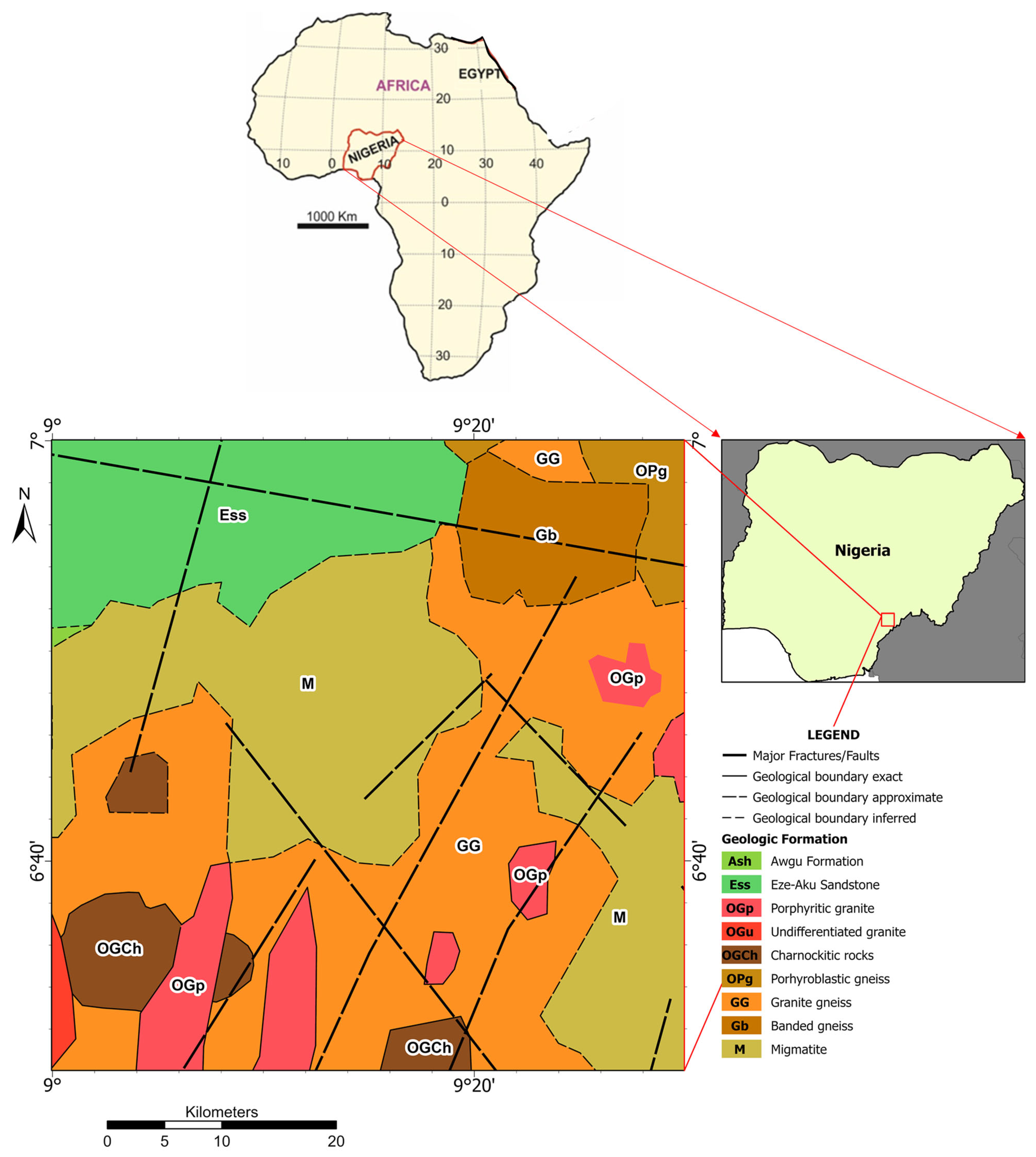
2. Location and Geology of the Investigated Area

The studied location was situated within the Precambrian Obudu basement complex (Figure 1), and it was located between longitude values of 9°00′ E and 9°30′ E and latitude values of 6°30′ N and 7°00′ N. According to [44], a series of tectono-thermal events with about three or more stages of distortion are responsible for the formation of the Nigerian basement complex. Three lithologic assemblages—the migmatite–gneiss complex, schist belts, and older granite sets—generally characterize the basement complex. In structurally regulated basins, the Cretaceous-Recent sedimentary sequence has been successfully maintained. The main rocks in the Nigerian basement complex are believed to be migmatite–gneiss complexes [45]. Age values related to the Kibaran ranged from 900 to 450 Ma, indicating the influence of the Pan-African occurrence that produced gneisses, migmatite, older granites, and connected lithological components [45].

There were no magmatic or depositional events that occurred during the middle-to-late Paleozoic era. Younger Jurassic granites are among the alkaline, anorogenic, shallow sub-volcanic intrusive materials that characterize the Mesozoic era. They are found in a north–south thin belt in the western part of the eastern region and extend northward into the Republic of Niger. One of Nigeria’s Precambrian basement outcrops is located in the Obudu Plateau, a section of the Bamenda Massif [46]. High-grade metamorphic rocks, including migmatized schists and gneisses that have been affected by granites, quartzo-feldspathic veins, and unmetamorphosed dolerites, are to blame for the region’s unusual lithology [46]. Amphibolites, metaquartzites, and metagabbro are also present in these rocks in traces. According to [47], the rocks in this area date to the Archaean, Eburnean, and Pan-African eras. Researchers arrived at the conclusion that the Southeast Nigerian basement evolutionary history is connected to the Pan-African mobile belt in Central Africa because of the relatively close agreement between the lithology of the rocks and ages of the Southeast Nigeria, Northern Cameroon, and Central African Fold Belt basement complexes [47]. The Adamawa-Yade and western Cameroon domain served as the active margin during the continent-to-continent collision that created to the Pan-Central African belt in Central Africa, whereas the northern Congo Craton border served as the passive margin [48]. According to [46], migmatitic gneiss, also known as garnet–sillimanite gneiss, garnet–hornblende gneiss, or simply migmatite gneiss, compose the majority of the OP.

3. Methodology

3.1. Two-Dimensional Magnetic Forward Problem

After carefully examining the magnetic anomaly expressions of horizontal cylinders [49], thin sheets [50], and spheres, [51,52] summarized the general new formula of the two-dimensional magnetic anomaly (T) profile for simple geometric bodies, which is defined as:

$$T_{(x_i,z)}=K\frac{A{z}^2+B\left(x_i-x_0\right)+C{\left(x_i-x_0\right)}^2}{{\left[{\left(x_i-x_0\right)}^2+z^2\right]}^{Sf}}, i=0, 1, 2, 3,\dots \dots \dots , N$$

(1)

where K is the amplitude coefficient, z is the depth of the buried body, and A, B, and C are described as follows:

$$A\left\{\begin{array}{c}3{sin}^2\theta -1\\ 2sin\theta \\ -cos\theta \\ cos\theta \\ \frac{cos\theta }{z}\end{array}, B\left\{\begin{array}{c}-3zsin\theta \\ -3zcos\theta \\ -3zsin\theta , C\\ 2zsin\theta \\ -sin\theta \end{array}\right.\right.\left\{\begin{array}{c}3{cos}^2\theta -1\\ -sin\theta \\ 2cos\theta \\ 0\end{array}\right.$$

• For a sphere (total field);
• For a sphere (vertical field);
• For a sphere (horizontal field);
• For a horizontal cylinder, FHD of thin sheet, and SHD of geological contact (all fields);
• For a thin sheet and FHD of geological contacts (all fields).

θ is the angle of effective magnetization [51,53] in the spheres. Additionally, ref [54] defines the cases of thin sheets and horizontal cylinders as follows: x₀ is the coordinate of the source body’s center, FHD and SHD are the first and second horizontal derivatives of the magnetic anomaly, respectively; N is the number of data points; and Sf is the shape factor, with values of 2.5 for spheres, 2 for horizontal cylinders, and 1 for thin sheets [55].

3.2. Magnetic Inverse Problem

In geophysics, the inversion technique is an optimization process aimed at identifying the model parameters of concealed geological features that are most suitable for explaining the measured data. To solve the inverse problem, it is necessary to perform this with an initial model [56]. This preliminary model can be established using drilling, other geophysical methods, and prior geological knowledge [57]. Every iteration step involves progressively refining the initial model until the theoretical and observed data are the best match.

According to the two-dimensional magnetic formula (Equation (1)), the model’s unidentified parameters are the origin’s location (x₀), depth (z), index angle (θ), shape factor (Sf), and amplitude coefficient (K). Due to its ease of use and speedy operation by merging fewer operators, the PSO technique was utilized to resolving the inverse problem. Furthermore, it is stable in terms of both numbers and mathematics. The model parameter values that would minimize the discrepancies between the collected field data and the theoretical model are determined using the following simple objective function:

$$Q=\frac{2{\sum }_{i=1}^N\left|T_i^m-T_i^c\right|}{{\sum }_{i=1}^N\left|T_i^m-T_i^c\right|+{\sum }_{i=1}^N\left|T_i^m-T_i^c\right|}$$

(2)

where N is the number of data points, $T_i^m$ is the observed magnetic anomaly at the point x_i, and $T_i^c$ is the approximated magnetic anomaly at the point x_i.

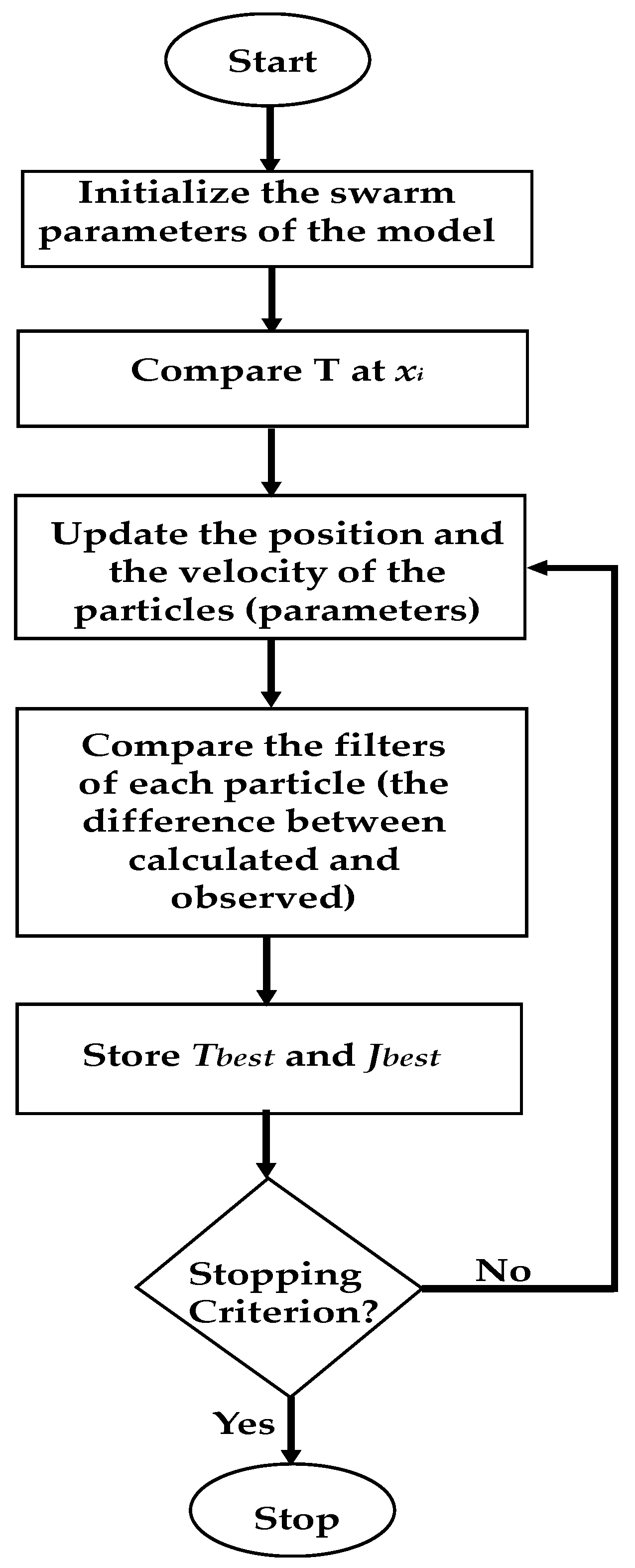
3.3. Particle Swarm Optimization

Ref [34] suggested the PSO technique as a global optimization algorithm. It depends on creatures (represented as particles) in the environment imitating natural processes, such as fish schooling and birds flocking. A point in M-dimensional space has an equivalent competitive solution for each particle in a PSO algorithm. In the inquiry space of the objective function, the computation is introduced freely and the initial solutions are established arbitrarily [58]. The PSO algorithm effectively guides researchers to achieving a global optimum value. The PSO algorithm’s main model structure is that the most likely answers are developed before the best ones. Figure 2 shows a basic flowchart. The PSO algorithm starts by assigning each particle in the swarm a random position and speed in the problem search space. Every bird, which represents a particle or model, has a velocity vector and a position vector that reflect the parameter value. PSO explains a swarm of particles (models) in an M-dimensional space. Each particle retains the position and speed of its previous optimal state. The best location of the swarm and the previous best position, often referred to as the Tbest model inhabited by the particle, are utilized to jointly estimate the speed modification of the particle at each iteration phase. The modified velocity is then utilized to calculate a new position for the particle using the Jbest model [59]. The following equations, according to [60], describe the update:

$$V_i^{k+1}=c_3{V}_i^k+c_{1}rand ()(T_{best}-P_i^{k+1})+c_{2}rand ()[(J_{best}-P_i^{k+1})P_i^{k+1}]=P_i^k+V_i^{k+1}$$

(3)

$$x_i^{k+1}=x_i^k+v_i^{k+1}$$

(4)

where $P_i^k$ is the current i model at the kth iteration, $v_i^k$ is the speed of the ith particle at the kth iteration, and rand() is an identical random number in the rang (0, 1). c₁ and c₂ are the positive consistent numbers that control individual and social behaviors [61]. c₃ is the inertial coefficient that controls the particle velocity. $x_i^k$ is the position of the particle i at the kth iteration.

The magnetic anomaly from Equation (1) is computed every iterative phase for each x_i using the PSO algorithm. To estimate the quality of the data fit at each iteration phase of the inversion process, the RMS is given as:

$$\mathrm{R}\mathrm{M}\mathrm{S}=\sqrt{\frac{{\sum }_{i=1}^N{\left[T_i^m\left(x_i\right)-T_i^c\left(x_i\right)\right]}^2}{N}}$$

(5)

This is taken as the misfit between the observed and theoretical anomalies.

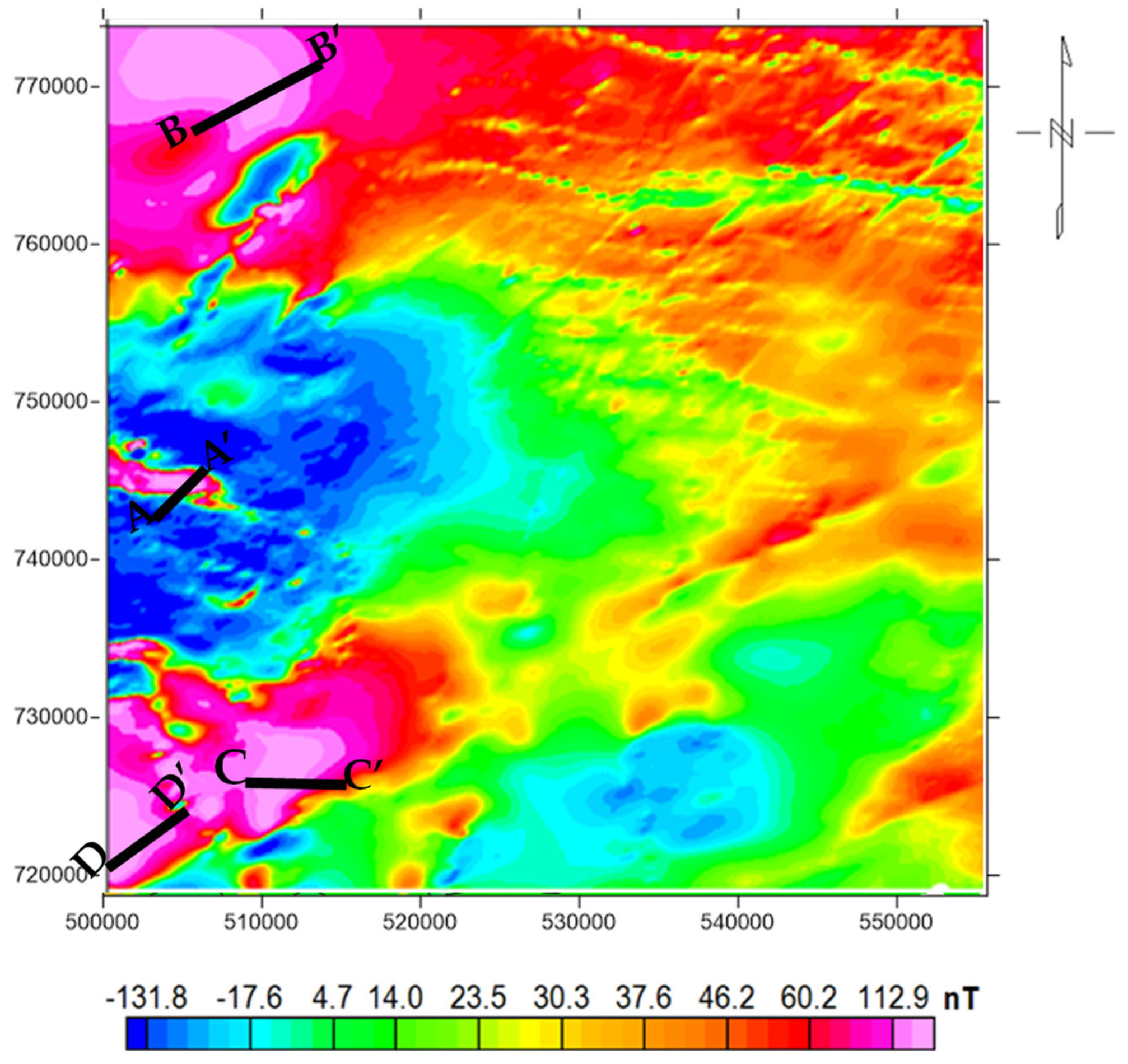
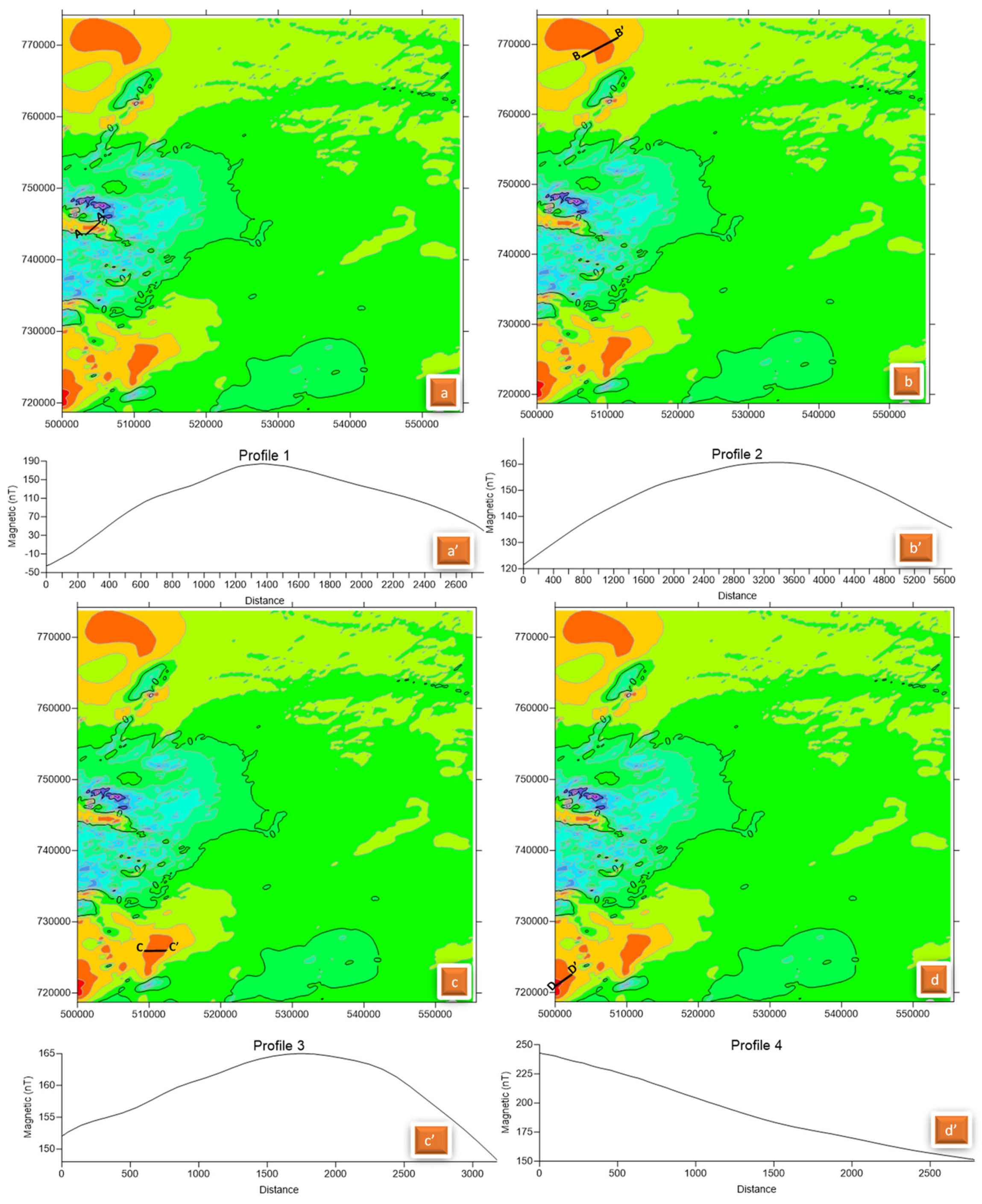
4. Data Acquisition and Selection of Profiles

The aero-magnetic data that were used in this work (Figure 3) were collected and filtered between 2005 and 2010 by Fugro Airborne Services, Canada. These data were collected by means of a Flux-Adjusting Surface Data Assimilation System with a flight-line space of 0.1 km, tie line space of 0.5 km, and terrain clearance ranging from 0.08–0.1 km along 826,000 lines. The mean total field, inclination value, and declination value were 32,851.9 nT, −14.6°, and −2.4°, respectively. The magnetic data have the potential to map small geologic anomalies, and when compared to the aero-magnetic data from 1970, they were found to be of good quality. In order to obtain associated PSO parameters, including the origin position (x₀), depth (z), amplitude coefficient (K), and index angle (θ), the profiles used in the PSO operation were carefully chosen across notable anomalies of the magnetic data (Figure 4).

5. Interpretation and Discussion of Results

The PSO algorithm was used for magnetic data interpretations over the Obudu Precambrian basement complex in Nigeria. The area that is situated in the eastern flank of Nigeria’s border with the Republic of Cameroon is predominantly composed of metamorphic rocks that have been invaded by unaltered granites, dolerites, and quartzo-feldspathic veins [3,46,62,63,64,65]. The profile of A–A’ (with a distance of 2600 m) and its related signature (Figure 4a’) were obtained from the magnetic data.

Table 1. Numerical results of magnetic anomaly for profile A–A’.

S/N	Parameter	Range	PSO Result	GA Result
1	K (nT)	0–3000	315.67	297.54
2	z (m)	200–1200	425.34	417.69
3	θ (°)	−90–90	43	47
4	Sf (dimensionless)	0.5–2.5	1.15	1.05
5	x0 (m)	1100–1900	1554.86	1527.97
6	RMS (nT)		6.43	8.59

displays the results of the inverted model parameters (depth, amplitude coefficient, index angle, shape factor, and location of origin) over A–A’. The optimum results of the model parameters from the magnetic anomaly are observed as K = 315.67 nT, z = 425.34 m, θ = 43°, Sf = 1.15, and x₀ = 1554.86 m.

Profile (B–B’) in Figure 4 shows the component of the magnetic anomaly with a profile length of 5600 m. The model parameters are displayed in

Table 2. Numerical results of magnetic anomaly for profile B–B’.

S/N	Parameter	Range	PSO Result	GA Result
1	K (nT)	0–3000	257.71	278.28
2	z (m)	200–1200	543.75	549.14
3	θ (°)	−90–90	54	50
4	Sf (dimensionless)	0.5–2.5	0.96	0.89
5	x0 (m)	2500–3800	3645.42	3654.87
6	RMS (nT)		4.81	6.28

, which were obtained from the observed geologic anomaly. Table 2 reveals the evaluated model parameters as K = 257.71 nT, z = 543.75 m, θ = 54°, Sf = 0.96, and x₀ = 3645.42 m. Furthermore, the parameters of the third anomaly (

Table 3. Numerical results of magnetic anomaly for profile C–C’.

S/N	Parameter	Range	PSO Result	GA Result
1	K (nT)	0−3000	189.53	208.35
2	z (m)	200–1200	560.87	569.26
3	θ (°)	−90–90	48	52
4	Sf (dimensionless)	0.5–2.5	1.2	1.13
5	x0 (m)	500–3000	1950	1962
6	RMS (nT)		5.95	9.62

) obtained from the profile length of 3000 m (Figure 4; profile C–C’) were K = 189.53 nT, z = 560.87 m, θ = 48, Sf = 1.2, and x₀ = 1950 m. The fourth magnetic anomaly profile with a length of 2500 m and associated signature (a’) (Figure 4) revealed the inverted model parameters (

Table 4. Numerical results of magnetic anomaly for profile D–D’.

S/N	Parameter	Range	PSO Result	GA Result
1	K (nT)	0−3000	247.23	219.59
2	z (m)	200–1200	394.16	384.15
3	θ (°)	−90–90	39	45
4	Sf (dimensionless)	0.5–2.5	1.26	0.97
5	x0 (m)	50–1250	165.41	170.57
6	RMS (nT)		8.92	11.53

) of 247.23 nT, 394.16 m, 39°, 1.26, and 165.41 m, respectively, for amplitude coefficient, depth, index angle, shape factor, and location of the origin over D–D’. It can be noticed that profile D–D’ (Figure 4d’) originates from the peak of the noticed magnetic anomaly and, as a result, the profile signature assumes the shape of a quarter cycle. From the obtained shape factor results involving the four models (Sf = 1.15, 0.96, 1.2, and 1.26), it can be established that the four magnetic anomalies are generated by thin sheets. Similar results were reported by [21] (Sf = 0.89 and 0.93) in their comparative study involving the application of PSO to real and synthetic data. On the contrary, Sf values of 2.5 and 2.0 were reported for the sphere and horizontal cylinder, respectively [21]. These geologic structures are created by the invasion of older granite suites by younger granite suites, resulting in a series of metamorphisms [66], folds, faults, and shear zones [67,68] linked to the Pan-African orogeny and succeeding post-orogenic events [67]. According to several published studies, geological structures within tectonically active regions act as depositional zones for igneous-related minerals and migratory pathways for hydrothermal fluids [69,70,71]. Magmatism and mineralization are linked, according to several investigations [3,45,69,71]. Therefore, it is believed that vast quantities of metallogenic minerals in the study area are under the influence of magmatic intrusions.

The validity of the PSO algorithm was tested on real data obtained from the Pima copper mine, United States of America, and the Hamrawein zone, Egypt [21]. The Pima copper mine field is characterized by minerals related to Laramide Paleozoic igneous activity [72]. The magnetic anomaly profile (696 m length) over a thin sheet-like feature is well-defined by these model parameters (K = 600 nT, z = 71.08 m, h = −47.83, Sf = 0.92, and x₀ = −0.49) [50]. The correlation between the measured and theoretical data, including drilling information [73], indicates a relatively strong match [50]. Similarly, the PSO algorithm was used for magnetic data acquired from Hamrawein, Egypt. This region is located at the western flank of the Red Sea and is dominated by sedimentary and metavolcanic rocks [74]. The observed anomalies were characterized by inverted model parameters of 507.64 nT, 623.05 m, 57.04°, 0.89, and 4255.98 m (amplitude coefficient, depth, index angle, shape factor, and location of origin, respectively) and 427.38 nT, 494.14 m, 37.27°, 0.93, and 14,823.96 m (amplitude coefficient, depth, index angle, shape factor, and location of origin, respectively) for the first and second anomalies [21]. Previous studies have shown the strong correlations of theoretical and observed anomalies [21]. Likewise, the PSO procedure, when compared with the very fast simulated annealing method (VFSAM), generated good results in a shorter time period [75].

The inversion outcomes for the four profiles (A–A’, B–B’, C–C’, and D–D’), presented in Table 1, Table 2, Table 3 and Table 4, utilizing the particle swarm optimization method were juxtaposed with those obtained through the genetic algorithm. This comparison reveals that the results achieved via the PSO approach exhibit greater stability and efficiency, primarily attributable to their lower root mean square (RMS) values.

6. Conclusions

In this research, the PSO algorithm was employed in approximating the distinctive model parameters (K, z, θ, x₀, and Sf) of the models. These models were generated from four profiles drawn for high-quality airborne magnetic data obtained from the Precambrian Obudu basement complex in Nigeria. Magnetic anomaly profile A–A’ with a distance of 2600 m generated inverted model parameters of K = 315.67 nT, z = 425.34 m, θ = 43°, Sf = 1.15, and x₀ = 1554.86 m. The second profile (B–B’) of a length of 5600 m had associated model parameters of K = 257.71 nT, z = 543.75 m, θ = 54°, Sf = 0.96, and x0 = 3645.42 m. Likewise, the parameters of the third anomaly obtained from a profile length of 3000 m (profile C–C’) were K = 189.53 nT, z = 560.87 m, θ = 48, Sf = 1.2, and x₀ = 1950 m. The fourth profile (with a length of 2500 m) that originated from the peak of the magnetic anomaly produced inverted model parameters of 247.23 nT, 394.16 m, 39°, 1.26, and 165.41 m, respectively, for the amplitude coefficient, depth, index angle, shape factor, and location of the origin. On the whole, the obtained shape factor values of the four models (Sf = 1.15, 0.96, 1.2, and 1.26) suggest the magnetic anomalies are initiated by thin sheets. The model results show that the PSO procedure is rapid, stable, and proficient for analyzing magnetic data for quantitative interpretations. The observed geological structures from the PSO results reveal depositional zones for igneous-related minerals and migratory pathways for hydrothermal fluids. As a result, it is believed that vast quantities of metallogenic minerals in the study area are associated with magmatic intrusions.

References

1. Ekwok, S.E.; Akpan, A.E.; Achadu, O.I.M.; Eze, O.E. Structural and lithological interpretation of aero-geophysical data in parts of the Lower Benue Trough and Obudu Plateau, Southeast Nigeria. Adv. Space Res. 2021, 68, 2841–2854. [Google Scholar] [CrossRef]
2. Ekwok, S.E.; Akpan, A.E.; Ebong, D.E. Enhancement and modelling of aeromagnetic data of some inland basins, southeastern Nigeria. J. Afr. Earth Sci. 2019, 155, 43–53. [Google Scholar] [CrossRef]
3. Ekwok, S.E.; Akpan, A.E.; Kudamnya, E.A. Exploratory mapping of structures controlling mineralization in Southeast Nigeria using high resolution airborne magnetic data. J. Afr. Earth Sci. 2020, 162, 103700. [Google Scholar] [CrossRef]
4. Ivakhnenkoa, O.P.; Abirova, R.; Logvinenkoc, A. New method for characterisation ofpetroleum reservoir fluid mineral deposits using magnetic analysis. Energy Procedia 2015, 76, 454–462. [Google Scholar] [CrossRef]
5. Eldosouky, A.M.; Ekwok, S.E.; Akpan, A.E.; Achadu, O.-I.M.; Pham, L.T.; Abdelrahman, K.; Gómez-Ortiz, D.; Alarifi, S.S. Delineation of structural lineaments of Southeast Nigeria using high resolution aeromagnetic data. Open Geosci. 2022, 14, 331–340. [Google Scholar] [CrossRef]
6. Eldosouky, A.M.; Ekwok, S.E.; Ben, U.C.; Ulem, C.A.; Abdelrahman, K.; Gomez-Ortiz, D.; Akpan, A.E.; George, A.M.; Pham, L.T. Appraisal of geothermal potentials of some parts of the Abakaliki Anticlinorium and adjoining areas (Southeast Nigeria) using magnetic data. Front. Earth Sci. 2023, 11, 1216198. [Google Scholar] [CrossRef]
7. Alfaifi, H.J.; Ekwok, S.E.; Ulem, C.A.; Eldosouky, A.M.; Qaysi, S.; Abdelrahman, K.; Andráš, P.; Akpan, A.E. Exploratory assessment of geothermal resources in some parts of the Middle Benue Trough of Nigeria using airborne potential field data. J. King Saud. Univ. Sci. 2023, 35, 102521. [Google Scholar] [CrossRef]
8. Abdelrahman, K.; Ekwok, S.E.; Ulem, C.A.; Eldosouky, A.M.; Al-Otaibi, N.; Hazaea, B.Y.; Hazaea, S.A.; Akpan, A.E. Exploratory Mapping of Geothermal Anomalies in the Neoproterozoic Arabian Shield, Saudi Arabia Using Magnetic Data. Minerals 2023, 13, 694. [Google Scholar] [CrossRef]
9. Gündoğdu, N.Y.; Candansayar, M.E.; Genç, E. Rescue archaeology application: Investigation of Kuriki mound archaeological area (Batman, SE Turkey) by using direct current resistivity and magnetic methods. J. Environ. Eng. Geophys. 2017, 22, 177–189. [Google Scholar] [CrossRef]
10. Abo-Ezz, E.R.; Essa, K.S. A least-squares minimization approach for model parameters estimate by using a new magnetic anomaly formula. Pure Appl. Geophys. 2016, 173, 1265–1278. [Google Scholar] [CrossRef]
11. Ben, U.C.; Ekwok, S.E.; Akpan, A.E.; Mbonu, C.C.; Eldosouky, A.M.; Abdelrahman, K.; Gómez-Ortiz, D. Interpretation of magnetic anomalies by simple geometrical structures using the manta-ray foraging optimization. Front. Earth Sci. 2022, 10, 849079. [Google Scholar] [CrossRef]
12. Ben, U.C.; Mbonu, C.C.; Thompson, C.E.; Ekwok, S.E.; Akpan, A.E.; Akpabio, I.; Eldosouky, A.M.; Abdelrahman, K.; Alzahrani, H.; Gómez-Ortiz, D.; et al. Investigating the applicability of the social spider optimization for the inversion of magnetic anomalies caused by dykes. J. King Saud. Univ. Sci. 2023, 35, 102569. [Google Scholar] [CrossRef]
13. Essa, K.S.; Elhussein, M. Interpretation of magnetic data through particle swarm optimization: Mineral exploration cases studies. Nat. Resour. Res. 2020, 29, 521–537. [Google Scholar] [CrossRef]
14. Abdelrahman, E.M.; Abo-Ezz, E.R.; Essa, K.S.; El-Araby, T.M.; Soliman, K.S. A new least-squares minimization approach to depth and shape determination from magnetic data. Geophys. Prospect. 2007, 55, 433–446. [Google Scholar] [CrossRef]
15. Abdelrahman, E.M.; Abo-Ezz, E.R.; Essa, K.S. Parametric inversion of residual magnetic anomalies due to simple geometric bodies. Explor. Geophys. 2012, 43, 178–189. [Google Scholar] [CrossRef]
16. Ku, C.C.; Sharp, J.A. Werner deconvolution for automated magnetic interpretation and its refinement using Marquardt’s inverse modeling. Geophysics 1983, 48, 754–774. [Google Scholar] [CrossRef]
17. Thompson, D.T. EULDPH—A new technique for making computer-assisted depth estimates from magnetic data. Geophysics 1982, 47, 31–37. [Google Scholar] [CrossRef]
18. Pilkington, M. Joint inversion of gravity and magnetic data for two-layer models. Geophysics 2006, 71, L35–L42. [Google Scholar] [CrossRef]
19. Abdelrahman, E.M.; El-Araby, H.M.; El-Araby, T.M.; Essa, K.S. A least-squares minimization approach to depth determination from magnetic data. Pure Appl. Geophys. 2003, 160, 1259–1271. [Google Scholar] [CrossRef]
20. Tlas, M.; Asfahani, J. Fair function minimization for interpretation of magnetic anomalies due to thin dikes, spheres and faults. J. Appl. Geophys. 2011, 75, 237–243. [Google Scholar] [CrossRef]
21. Essa, K.S.; Elhussein, M. PSO (Particle Swarm Optimization) for interpretation of magnetic anomalies caused by simple geometrical structures. Pure Appl. Geophys. 2018, 175, 3539–3553. [Google Scholar] [CrossRef]
22. Van den Bergh, F.; Engelbrecht, A.P. A Cooperative approach to particle swarm optimization. IEEE Trans. Evol. Comput. 2004, 8, 225–239. [Google Scholar] [CrossRef]
23. Boschetti, F.; Denith, M.C.; List, R.D. Inversion of potential field data by genetic algorithms. Geophys. Prospect. 1997, 45, 461–478. [Google Scholar] [CrossRef]
24. Biswas, A. Interpretation of residual gravity anomaly caused by a simple shaped body using very fast simulated annealing global optimization. Geosci. Front. 2015, 6, 875–893. [Google Scholar] [CrossRef]
25. Ekinci, Y.L.; Balkaya, Ç.; Göktürkler, G.; Turan, S. Model parameter estimations from residual gravity anomalies due to simple-shaped sources using differential evolution algorithm. J. Appl. Geophys. 2016, 129, 133–147. [Google Scholar] [CrossRef]
26. Balkaya, C.; Ekinci, Y.L.; Göktürkler, G.; Turan, S. 3D non-linear inversion of magnetic anomalies caused by prismatic bodies using differential evolution algorithm. J. Appl. Geophys. 2017, 136, 372–386. [Google Scholar] [CrossRef]
27. Biswas, A. Inversion of source parameters from magnetic anomalies for mineral/ore deposits exploration using global optimization technique and analysis of uncertainty. Nat. Resour. Res. 2018, 27, 77–107. [Google Scholar] [CrossRef]
28. Essa, K.S.; Elhussein, M. Gravity Data Interpretation Using New Algorithms: A Comparative Study. In Gravity-Geoscience Applications, Industrial Technology and Quantum Aspect; Zouaghi, Z., Ed.; InTech: Rijeka, Croatia, 2018. [Google Scholar]
29. Srivastava, S.; Datta, D.; Agarwal, B.N.P.; Mehta, S. Applications of ant colony optimization in determination of source parameters from total gradient of potential fields. Near Surf. Geophys. 2014, 12, 373–389. [Google Scholar] [CrossRef]
30. Di Maio, R.; Rani, P.; Piegari, E.; Milano, L. Selfpotential data inversion through a genetic-price algorithm. Comput. Geosci. 2016, 94, 86–95. [Google Scholar] [CrossRef]
31. Holland, J.H. Adaptation in Natural and Artificial Systems; University of Michigan Press: Ann Arbor, MI, USA, 1975. [Google Scholar]
32. Kirkpatrick, S.; Gelatt, C.D.; Vecchi, M.P. Optimization by Simulated Annealing. Science 1983, 220, 671–680. [Google Scholar] [CrossRef]
33. Storn, R.; Price, K. Differential Evolution—A Simple and Efficient Heuristic for Global Optimization over Continuous Spaces. J. Glob. Optim. 1997, 11, 341–359. [Google Scholar] [CrossRef]
34. Kennedy, J.; Eberhart, R. Particle Swarm Optimization. In Proceedings of the IEEE International Conference on Neural Networks, Perth, WA, Australia, 27 November–1 December 1995; IEEE Service Center: PiscatawaY, NJ, USA, 1995. lV. pp. 1942–1948. [Google Scholar]
35. Mishra, S.; Pant, M. Particle Swamp Optimization: A Hybrid Swarm Intelligence Algorithm. Procedia Comput. Sci. 2017, 115, 453–460. [Google Scholar]
36. Eberhart, R.C.; Shi, Y. Particle Swarm Optimization: Developments, Applications and Resources. In Proceedings of the Congress on Evolutionary Computation, Seoul, Republic of Korea, 27–30 May 2001; pp. 81–86. [Google Scholar]
37. Toushmalani, R. Gravity inversion of a fault by particle swarm optimization (PSO). Springer Plus 2013, 2, 315. [Google Scholar] [CrossRef]
38. Juang, C.F. A hybrid genetic algorithm and particle swarm optimization for recurrent network design. IEEE Trans. Syst. Man Cybern. Part B 2004, 34, 997–1006. [Google Scholar] [CrossRef]
39. Robinson, J.; Rahamat-Samii, Y. Particle swarm optimization in electromagnetic. IEEE Trans. Antennas Propag. 2004, 52, 397–407. [Google Scholar] [CrossRef]
40. Cedeno, W.; Agrafiotis, D.K. Using particle swarms for the development of QSAR models based on K-nearest neighbor and kernel regression. J. Comput. Aided Mol. Des. 2003, 17, 255–263. [Google Scholar] [CrossRef]
41. Donelli, M.; Franceschini, G.; Martini, A.; Mass, A. An integrated multiscaling strategy based on a particle swarm algorithm for inverse scattering problems. IEEE Trans. Geosci. Remote Sens. 2006, 44, 298–312. [Google Scholar] [CrossRef]
42. Wachowiak, M.P.; Smolıkova, R.; Zheng, Y.; Zurada, J.M.; Elmaghraby, A.S. An approach to multimodal biomedical image registration utilizing particle swarm optimization. IEEE Trans. Evol. Comput. 2004, 8, 289–301. [Google Scholar] [CrossRef]
43. Chau, W.K. Application of a Particle Swarm Optimization Algorithm to Hydrological Problems. In Water Resources Research Progress; Robinson, L.N., Ed.; Nova Science Publishers Inc.: New York, NY, USA, 2008; pp. 3–12. [Google Scholar]
44. Rahaman, M.A.; Lancelot, J.R. Continental Crust Evolution in SW Nigeria: Constraints from U/Pb dating of Pre-Pan-African Gneisses. In Rapport D’activite 1980–1984 Documents et Travaux du Centre Geologique et Geophysique de Montpellier; Universitédes Sciences et Techniques du Languedoc: Montpellier, France, 1984; pp. 41–50. [Google Scholar]
45. Haruna, I.V. Review of the Basement Geology and Mineral Belts of Nigeria. J. Appl. Geol. Geophys. 2017, 5, 37–45. [Google Scholar]
46. Agbi, I.; Ekwueme, B.N. Preliminary review of the geology of the hornblende biotite gneisses of Obudu Plateau Southeastern Nigeria. Glob. J. Geol. Sci. 2018, 17, 75–83. [Google Scholar] [CrossRef]
47. Ukwang, E.E.; Ekwueme, B.N.; Kröner, A. Single zircon evaporation ages: Evidence for the Mesoproterozoic crust in the southeastern Nigerian basement complex. Chin. J. Geochem. 2012, 31, 48–54. [Google Scholar] [CrossRef]
48. Toteu, S.F.; Penaye, J.; Djomani, Y.P. Geodynamic evolution of the Pan-African belt in Central Africa with special reference to Cameroon. Can. J. Earth Sci. 2004, 41, 73–85. [Google Scholar] [CrossRef]
49. Rao, T.K.S.P.; Subrahmanyam, M.; Srikrishna Murthy, A. Nomograms for the direct interpretation of magnetic anomalies due to long horizontal cylinders. Geophysics 1986, 51, 2156–2159. [Google Scholar] [CrossRef]
50. Gay, P. Standard curves for interpretation of magnetic anomalies over long tabular bodies. Geophysics 1963, 28, 161–200. [Google Scholar] [CrossRef]
51. Rao, T.; Subrahmanyam, M. Characteristic curves for the inversion of magnetic-anomalies of spherical ore bodies. Pure Appl. Geophys. 1988, 126, 69–83. [Google Scholar]
52. Abdelrahman, E.M.; Essa, K.S. A new method for depth and shape determinations from magnetic data. Pure Appl. Geophys. 2015, 172, 439–460. [Google Scholar] [CrossRef]
53. Rao, B.S.R.; Murthy, I.V.R.; Rao, C.V. A computer program for interpreting vertical magnetic anomalies of spheres and horizontal cylinders. Pure Appl. Geophys. 1973, 110, 2056–2065. [Google Scholar] [CrossRef]
54. Gay, P. Standard curves for the interpretation of magnetic anomalies over long horizontal cylinders. Geophysics 1965, 30, 818–828. [Google Scholar] [CrossRef]
55. Abdelrahman, E.M.; Essa, K.S. Magnetic interpretation using a least-squares, depth-shape curves method. Geophysics 2005, 70, L23–L30. [Google Scholar] [CrossRef]
56. Lines, L.R.; Treitel, S. A review of least-squares inversion and its application to geophysical problems. Geophys. Prospect. 1984, 32, 159–186. [Google Scholar] [CrossRef]
57. Zhdanov, M.S. Geophysical Inversion Theory and Regularization Problems; Elsevier: Amsterdam, The Netherlands, 2002; p. 633. [Google Scholar]
58. He, J.; Guo, H. A modified particle swarm optimization algorithm. Telkomnika 2013, 11, 6209–6215. [Google Scholar] [CrossRef]
59. Sen, M.K.; Stoffa, P.L. Global Optimization Methods in Geophysical Inversion; Cambridge University Press: Cambridge, UK, 2013; p. 279. [Google Scholar]
60. Sweilam, N.H.; El-Metwally, K.; Abdelazeem, M. Self potential signal inversion to simple polarized bodies using the particle swarm optimization method: A visibility study. J. Appl. Geophys. 2007, 6, 195–208. [Google Scholar]
61. Parsopoulos, K.E.; Vrahatis, M.N. Recent approaches to global optimization problems through particle swarm optimization. Nat. Comput. 2002, 1, 235–306. [Google Scholar] [CrossRef]
62. Ekwok, S.E.; Akpan, A.E.; Achadu, O.-I.M.; Thompson, C.E.; Eldosouky, A.M.; Abdelrahman, K.; Andráš, P. Towards understanding the source of brine mineralization in Southeast Nigeria: Evidence from high-resolution airborne magnetic and gravity data. Minerals 2022, 12, 146. [Google Scholar] [CrossRef]
63. Ekwok, S.E.; Akpan, A.E.; Achadu, O.I.M.; Ulem, C.A. Implications of tectonic anomalies from potential feld data in some parts of Southeast Nigeria. Environ. Earth Sci. 2022, 81, 6. [Google Scholar] [CrossRef]
64. Ekwok, S.E.; Akpan, A.E.; Ebong, E.D.; Eze, O.E. Assessment of depth to magnetic sources using high resolution aeromagnetic data of some parts of the Lower Benue Trough and adjoining areas, Southeast Nigeria. Adv. Space Res. 2021, 67, 2104–2119. [Google Scholar] [CrossRef]
65. Ekwok, S.E.; Akpan, A.E.; Kudamnya, E.A.; Ebong, D.E. Assessment of groundwater potential using geophysical data: A case study in parts of Cross River State, south-eastern Nigeria. Appl. Water Sci. 2020, 10, 144. [Google Scholar] [CrossRef]
66. Nwankwo, L.I. Structural styles in the Precambrian Basement Complex of southeastern Nigeria. J. Afr. Earth Sci. 2009, 53, 73–86. [Google Scholar]
67. Ajibade, A.C.; Oyawoye, M.O.; Rahaman, M.A.; Adekeye, O.A. Petrology of migmatites of the Obudu Plateau, Nigeria. J. Afr. Earth Sci. 2010, 56, 23–30. [Google Scholar]
68. Asouzu, E.C.; Onyeagocha, A.C. Geology and mineralization of the Obudu area of southeastern Nigeria. J. Afr. Earth Sci. 2013, 86, 20–34. [Google Scholar]
69. Airo, M.L. Aeromagnetic and aeroradiometric response to hydrothermal alteration. Surv. Geophys. 2002, 23, 273–302. [Google Scholar] [CrossRef]
70. United States Geological Survey (USGS). Setting and Origin of Iron Oxide-Copper-Cobalt-Gold-Rare Earth Element Deposits of Southeast Missouri. 2013. Available online: http://minerals.usgs.gov/east/semissouri/index.html (accessed on 5 June 2023).
71. Geological Survey of Canada (GSC). Airborne Geophysical Survey, Mount Milligan area, British Columbia (NTS 93 O/4W, N/1, N/2E); GSC Open File 2535; GSC: Montreal, Canada, 1992.
72. Shafiqullah, M.; Langlois, J.D. The Pima Mining District Arizona—A Geochronologic Update. In New Mexico Geological Society Guidebook 29th Annual Fall Field Conference Guidebook; New Mexico Geological Society: Boulder, CO, USA, 1978; pp. 321–327. [Google Scholar]
73. Abdelrahman, E.M.; Sharafeldin, S.M. An iterative least-squares approach to depth determination from residual magnetic anomalies due to thin dikes. J. Appl. Geophys. 1996, 34, 213–220. [Google Scholar] [CrossRef]
74. Salem, A.; Aboud, E.; Elsirafy, A.; Ushijima, K. Structural mapping of Quseir area, northern Red Sea, Egypt, using high-resolution aeromagnetic data. Earth Planets Space 2005, 57, 761–765. [Google Scholar] [CrossRef]
75. Biswas, A.; Parija, M.P.; Kumar, S. Global nonlinear optimization for the interpretation of source parameters from otal gradient of gravity and magnetic anomalies caused by thin dyke. Ann. Geophys. 2017, 60, G0218. [Google Scholar] [CrossRef]
Figure 1. Location and geologic maps of the study area.
Minerals 13 01209 g001
Figure 2. Flowchart of the PSO algorithm applied to magnetic anomalies’ interpretations.
Minerals 13 01209 g002
Figure 3. Total magnetic intensity data showing locations of profiles.
Minerals 13 01209 g003
Figure 4. Profiles (aa’), (bb’), (cc’), and (dd’), and related signatures (a’), (b’), (c’), and (d’), respectively, obtained from the magnetic data.
Minerals 13 01209 g004