
Geochemistry as a Clue for Paleoweathering and Provenance of Southern Apennines Shales (Italy): A Review


Abstract
:1. Introduction
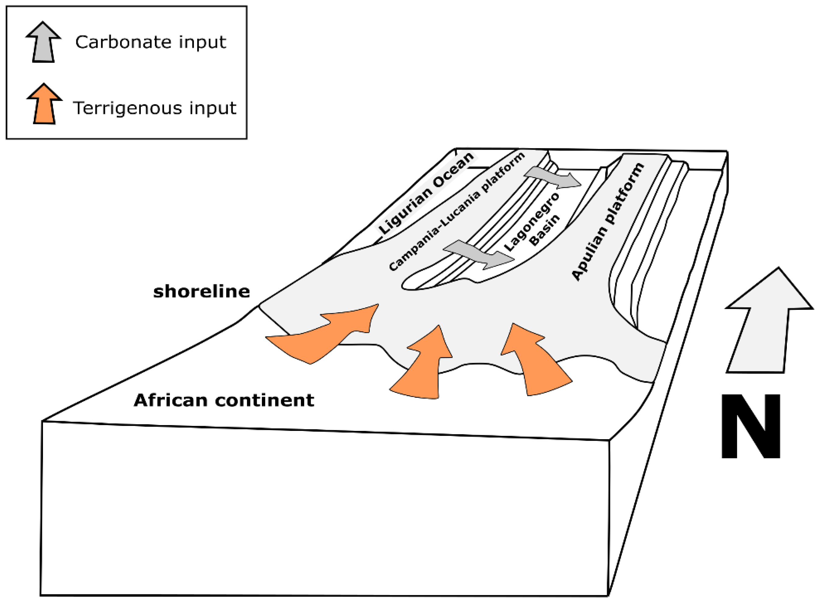
2. Geological Framework
3. Sampling and Analytical Methods
4. Results and Discussion
4.1. Mineralogy and Geochemistry
4.2. Factors Affecting the Distribution of Elements
4.3. Paleoweathering
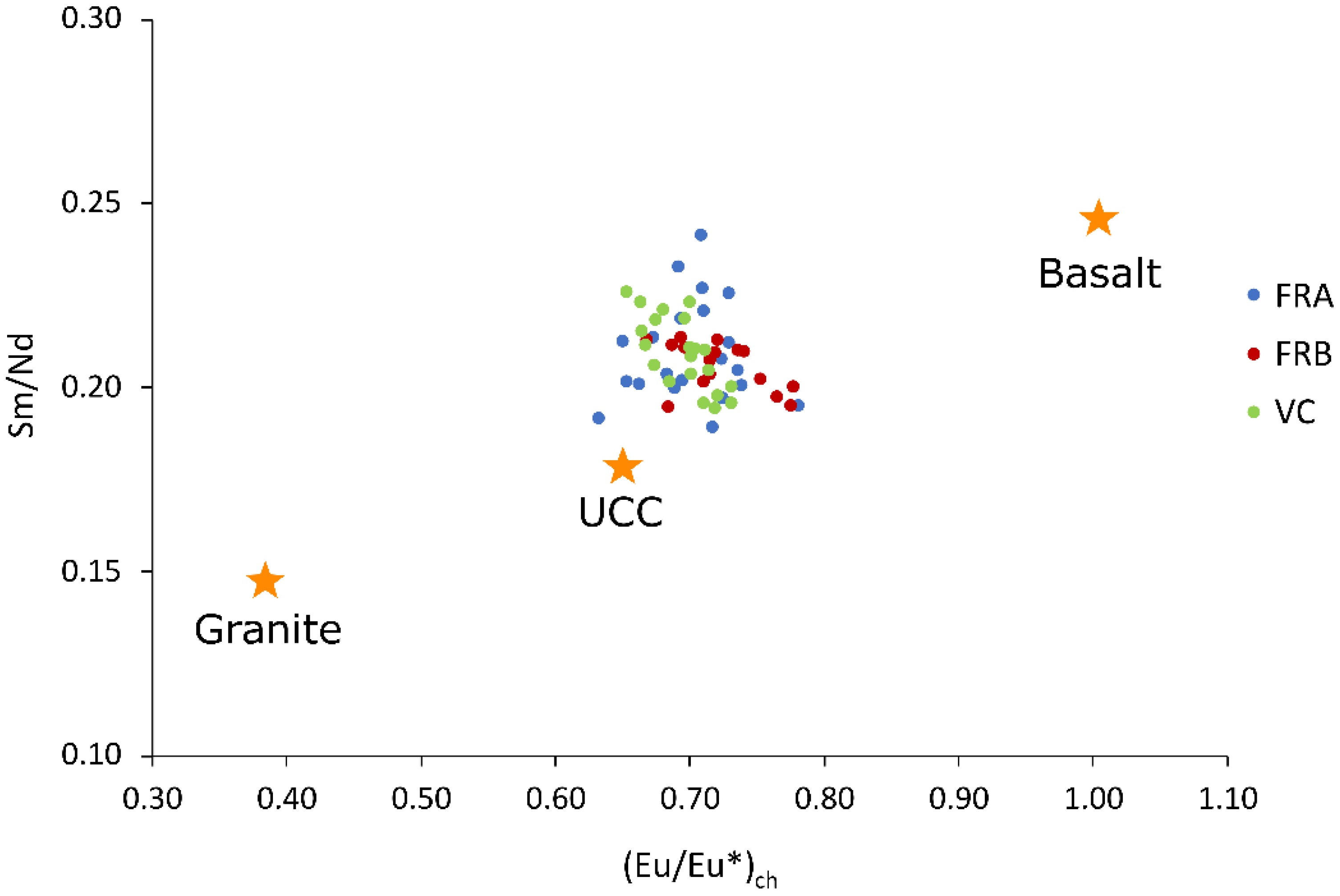
4.4. Provenance
5. Conclusions
Author Contributions
Funding
Data Availability Statement
Conflicts of Interest
References
- Taylor, S.R.; McLennan, S.M. The Continental Crust: Its Composition and Evolution; Blackwell: Oxford, UK, 1985. [Google Scholar]
- McLennan, S.M.; Hemming, S.; McDaniel, D.K.; Hanson, G.N. Geochemical approaches to sedimentation, provenance, and tectonics. Geol. Soc. Am. Spec. Pap. 1993, 284, 21–40. [Google Scholar]
- Mongelli, G.; Critelli, S.; Perri, F.; Sonnino, M.; Perrone, V. Sedimentary recycling, provenance and paleoweathering from chemistry and mineralogy of Mesozoic continental red bed mudrocks, Peloritani Mountains, Southern Italy. Geochem. J. 2006, 40, 197–209. [Google Scholar] [CrossRef] [Green Version]
- Fedo, C.M.; Eriksson, K.A.; Krogstad, E.J. Geochemistry of shales from the Archean (~3.0 Ga) Buhwa Greenstone Belt, Zimbabwe: Implications for provenance and source-area weathering. Geochim. Cosmochim. Acta 1996, 60, 1751–1763. [Google Scholar] [CrossRef]
- Hassan, S.; Ishiga, H.; Roser, B.P.; Do Zen, K.; Naka, T. Geochemistry of Permian–Triassic shales in the Salt Range, Pakistan: Implications for provenance and tectonism at the Gondwana margin. Chem. Geol. 1999, 158, 293–314. [Google Scholar] [CrossRef]
- Bauluz, B.; Mayayo, M.J.; Fernandez-Nieto, C.; Gonzales Lopez, J.M. Geochemistry of Precambrian and Paleozoic siliciclastic rocks from the Iberian Range (NE Spain): Implications for source-area weathering, sorting, provenance, and tectonic setting. Chem. Geol. 2000, 168, 135–150. [Google Scholar] [CrossRef]
- Cullers, R.L.; Podkovyrov, V.N. Geochemistry of the Mesoproterozoic Lakhanda shales in southeastern Yakutia, Russia: Implications for mineralogical and provenance control, and recycling. Precambrian Res. 2000, 104, 77–93. [Google Scholar] [CrossRef]
- Condie, K.C.; Lee, D.; Farmer, G.L. Tectonic setting and provenance of the Neoproterozoic Uinta Mountain and Big Cottonwood groups, northern Utah: Constraints from geochemistry, Nd isotopes, and detrital modes. Sediment. Geol. 2001, 141, 443–464. [Google Scholar] [CrossRef]
- Mongelli, G. Rare earth elements in Oligo-Miocenic pelitic sediments from Lagonegro basin, Southern Apennines, Italy: Implication for provenance and source area weathering. Int. J. Earth Sci. 2004, 93, 612–620. [Google Scholar] [CrossRef]
- Sinisi, R.; Mongelli, G.; Mameli, P.; Oggiano, G. Did the Variscan relief influence the Permian climate of Mesoeurope? Insights from geochemical and mineralogical proxies from Sardinia (Italy). Palaeogeogr. Palaeoclimatol. Palaeoecol. 2014, 396, 132–154. [Google Scholar] [CrossRef]
- Mameli, P.; Mongelli, G.; Sinisi, R.; Oggiano, G. Weathering products of a dismantled Variscan basement. Minero-chemical proxies to insight on Cretaceous palaeogeography and Late Neogene palaeoclimate of Sardinia (Italy). Front. Earth Sci. 2020, 8, 290. [Google Scholar] [CrossRef]
- Nesbitt, H.W.; Young, G.M. Early Proterozoic climates and plate motions inferred from major element chemistry of lutites. Nature 1982, 299, 715–717. [Google Scholar] [CrossRef]
- Harnois, L. The CIW index: A new chemical index of weathering. Sediment. Geol. 1988, 55, 319–322. [Google Scholar] [CrossRef]
- Fedo, C.M.; Eriksson, K.A.; Blenkinsop, T.G. Geologic history of the Archean Buhwa Greenstone Belt and surrounding granite–gneiss terrane, Zimbabwe, with implications for the evolution of the Limpopo Belt. Can. J. Earth Sci. 1995, 32, 1977–1990. [Google Scholar] [CrossRef]
- Perri, F. Reconstructing chemical weathering during the Lower Mesozoic in the Western-Central Mediterranean area: A review of geochemical proxies. Geol. Mag. 2018, 155, 944–954. [Google Scholar] [CrossRef]
- Perri, F. Chemical weathering of crystalline rocks in contrasting climatic conditions using geochemical proxies: An overview. Palaeogeogr. Palaeoclimatol. Palaeoecol. 2020, 556, 109873. [Google Scholar] [CrossRef]
- Sheldon, N.D.; Retallack, G.J.; Tanaka, S. Geochemical climofunctions from North American soils and application to paleosols across the Eocene-Oligocene boundary in Oregon. J. Geol. 2002, 110, 687–696. [Google Scholar] [CrossRef] [Green Version]
- Rasmussen, C.; Tabor, N.J. Applying a quantitative pedogenic energy model across a range of environmental gradients. Soil Sci. Soc. Am. J. 2007, 71, 1719–1729. [Google Scholar] [CrossRef]
- Lukens, W.E.; Nordt, L.C.; Stinchcomb, G.E.; Driese, S.G.; Tubbs, J.D. Reconstructing pH of paleosols using geochemical proxies. J. Geol. 2018, 126, 427–449. [Google Scholar] [CrossRef]
- Lukens, W.E.; Stinchcomb, G.E.; Nordt, L.C.; Kahle, D.J.; Driese, S.G.; Tubbs, J.D. Recursive partitioning improves paleosol proxies for rainfall. Am. J. Sci. 2019, 319, 819–845. [Google Scholar] [CrossRef]
- Nordt, L.C.; Driese, S.D. New weathering index improves paleorainfall estimates from Vertisols. Geology 2010, 38, 407–410. [Google Scholar] [CrossRef]
- Nordt, L.C.; Driese, S.G. A modern soil characterization approach to reconstructing physical and chemical properties of paleo-Vertisols. Am. J. Sci. 2010, 310, 37–64. [Google Scholar] [CrossRef]
- Stinchcomb, G.E.; Nordt, L.C.; Driese, S.G.; Lukens, W.E.; Williamson, F.C.; Tubbs, J.D. A data-driven spline model designed to predict paleoclimate using paleosol geochemistry. Am. J. Sci. 2016, 316, 746–777. [Google Scholar] [CrossRef]
- Knott, S.D. The Liguride complex of southern Italy—A Cretaceous to Paleogene accretionary wedge. Tectonophysics 1987, 142, 217–226. [Google Scholar] [CrossRef]
- Monaco, C.; Tortorici, L. Tectonic role of ophiolite-bearing terranes in the development of the Southern Apennines orogenic belt. Terra Nova 1995, 7, 153–160. [Google Scholar] [CrossRef]
- Pescatore, T.; Renda, P.; Schiattarella, M.; Tramutoli, M. Stratigraphic and structural relationships between Meso-Cenozoic Lagonegro basin and coeval carbonate platforms in southern Apennines, Italy. Tectonophysics 1999, 315, 269–286. [Google Scholar] [CrossRef]
- Ogniben, L. Schema introduttiva alla geologia del confine Calabro-Lucano. Mem. Soc. Geol. Ital. 1969, 8, 453–763. [Google Scholar]
- Mostardini, F.; Merlini, S. Appennino Centro. Meridionale e Proposta di Modello Strutturale. Mem. Soc. Geol. Ital. 1986, 35, 177–202. [Google Scholar]
- Pescatore, T.; Renda, P.; Tramutoli, M. Relationship between the Lagonegro and Silicidi formations of the middle valley of the Basento River, Lucca, Southern Apennines. Mem. Soc. Geol. Ital. 1988, 41, 353–361. [Google Scholar]
- Marsella, E.; Bally, A.W.; D’Argenio, B.; Cippitelli, G.; Pappone, G. Tectonic history of the Lagonegro Domain and Southern Apennine thrust belt evolution. Tectonophysics 1995, 252, 307–330. [Google Scholar] [CrossRef]
- Fiore, S.; Piccarreta, G.; Santaloia, F.; Santarcangelo, R.; Tateo, F. The Flysch Rosso shales from the southern Apennines, Italy. 1. Mineralogy and geochemistry. Per. Mineral. 2000, 69, 63–68. [Google Scholar]
- Mongelli, G. Trace elements distribution and mineralogical composition in the <2-μm size fraction of shales from the Southern Apennines, Italy. Mineral. Petrol. 1995, 53, 103–114. [Google Scholar]
- Caggianelli, A.; Fiore, S.; Mongelli, G.; Salvemini, A. REE distribution in the clay fraction of pelites from the southern Apennines, Italy. Chem. Geol. 1992, 99, 253–263. [Google Scholar] [CrossRef]
- Franzini, M.; Leoni, L.; Saitta, M. A simple method to evaluate the matrix effects in X-ray fluorescence analysis. X-ray Spectrom. 1972, 1, 151–154. [Google Scholar] [CrossRef]
- Franzini, M.; Leoni, L.; Saitta, M. Revisione di una metodologia analitica per fluorescenza-X, basata sulla correzione completa degli effetti di matrice Rend. Soc. Ital. Mineral. Petrol. 1975, 31, 365–378. [Google Scholar]
- Leoni, L.; Saitta, M. Determination of yttrium and niobium on standard silicate rocks by X-ray fluorescence analyses Rend. Soc. Ital. Mineral. Petrol. 1976, 32, 497–510. [Google Scholar]
- Govindaraju, K.; Mevelle, G. Fully automated dissolution and separation methods for inductively coupled plasma atomic emission spectrometry rock analysis. Application to the determination of rare earth elements. Plenary lecture. J. Anal. Atom. Spectrom. 1987, 2, 615–621. [Google Scholar]
- Mongelli, G. Ce-anomalies in the textural components of Upper Cretaceous karst bauxites from the Apulian carbonate platform (southern Italy). Chem. Geol. 1997, 140, 69–79. [Google Scholar] [CrossRef]
- Herron, M.M. Mineralogy from geochemical well logging. J. Sedim. Petrol. 1986, 58, 820–829. [Google Scholar] [CrossRef]
- Fiore, S.; Mongelli, G. Hypothesis on the genesis of day minerals in the fine fraction of «Argille varicolori» from Andretta (southem Apennines). Miner. Petrog. Acta 1991, 34, 183–190. [Google Scholar]
- Di Leo, P.; Dinelli, E.; Mongelli, G.; Schiattarella, M. Geology and geochemistry of Jurassic pelagic sediments, Scisti silicei Formation, southern Apennines. Italy Sed. Geol. 2002, 150, 229–246. [Google Scholar] [CrossRef]
- Mongelli, G.; Dinelli, E. The geochemistry of shales from the “Frido Unit”, Liguride Complex, Lucanian Apennines, Italy: Implications for provenance and tectonic setting. Ofiotiti 2001, 26, 457–466. [Google Scholar]
- Davis, J.C. Statistics and Data Analysis in Geology; John Wiley & Sons: New York, NY, USA, 1986. [Google Scholar]
- Ahmadnejad, F.; Mongelli, G. Geology, geochemistry, and genesis of REY minerals of the late Cretaceous karst bauxite deposits, Zagros Simply Folded Belt, SW Iran: Constraints on the ore-forming process. J. Geochem. Explor. 2022, 240, 107030. [Google Scholar] [CrossRef]
- Ferhaoui, S.; Kechiched, R.; Bruguier, O.; Sinisi, R.; Kocsis, L.; Mongelli, G.; Bosch, D.; Ameur Zaimeche, O.; Laouar, R. Rare earth elements plus yttrium (REY) in phosphorites from the Tébessa region (Eastern Algeria): Abundance, geochemical distribution through grain size fractions, and economic significance. J. Geochem. Explor. 2022, 241, 107058. [Google Scholar] [CrossRef]
- Liu, Y.H.; Lee, D.C.; You, C.F.; Takahata, N.; Iizuka, Y.; Sano, Y.; Zhou, C. In-situ U–Pb dating of monazite, xenotime, and zircon from the Lantian black shales: Time constraints on provenances, deposition and fluid flow events. Precambrian Res. 2020, 349, 105528. [Google Scholar] [CrossRef]
- Perri, F.; Critelli, S.; Martín-Martín, M.; Montone, S.; Amendola, U. Unravelling hinterland and offshore palaeogeography from pre-to-syn-orogenic clastic sequences of the Betic Cordillera (Sierra Espuña), Spain. Palaeogeogr. Palaeoclimatol. Palaeoecol. 2017, 468, 52–69. [Google Scholar] [CrossRef] [Green Version]
- Abedini, A.; Mongelli, G.; Khosravi, M.; Sinisi, R. Geochemistry and secular trends in the middle–late Permian karst bauxite deposits, northwestern Iran. Ore Geol. Rev. 2020, 124, 103660. [Google Scholar] [CrossRef]
- Michel, L.A.; Sheldon, N.D.; Myers, T.S.; Tabor, N.J. Assessment of pretreatment methods on CIA-K and CALMAG indices and the effects on paleoprecipitation estimates. Palaeogeogr. Palaeoclimatol. Palaeoecol. 2022, 601, 111102. [Google Scholar] [CrossRef]
- Maynard, J.B. Chemistry of modern soils as a guide to interpreting Precambrian paleosols. J. Geol. 1992, 100, 279–289. [Google Scholar] [CrossRef]
- Viers, J.; Wasserburg, G.J. Behavior of Sm and Nd in a lateritic soil profile. Geochim. Et Cosmochim. Acta 2004, 68, 2043–2054. [Google Scholar] [CrossRef]
- Condie, K.C. Chemical composition and evolution of the upper continental crust: Contrasting results from surface samples and shales. Chem. Geol. 1993, 104, 1–37. [Google Scholar] [CrossRef]
- McLennan, S.M.; Taylor, S.R. Sedimentary rocks, and crustal evolution: Tectonic setting and secular trends. J. Geol. 1991, 99, 1–21. [Google Scholar] [CrossRef]


| Locality | Lithology | Age | Formation | Sample Code | No. of Samples | Mineralogy |
|---|---|---|---|---|---|---|
| Campomaggiore and Vaglio di Basilicata [31] | shales interbedded with siltstones and radiolarian cherts | Late Cretaceous–Medium Miocene | Red Flysch Fm. | FRA | 22 | Illite > Smectite > Kaolinite, Chlorite > Quartz > Calcite |
| Monteverde village [32] | shales with minor calcarenite levels | Late Cretaceous–Medium Miocene | Red Flysch Fm. | FRB | 16 | Smectite > Illite > Kaolinite, Chlorite > Quartz > Calcite |
| Tolve village [3,33] | pelitic sequence with rare limestones and marly limestones | Upper Cretaceous–Lower Eocene | Argille Varicolori Fm. | VC | 16 | Illite > Smectite > Kaolinite, Chlorite > Quartz > Calcite |
| SiO2 | TiO2 | Al2O3 | Fe2O3 | MnO | MgO | CaO | Na2O | K2O | P2O5 | LOI | |
|---|---|---|---|---|---|---|---|---|---|---|---|
| FRA3 | 63.4 | 0.69 | 14.4 | 6.03 | 0.77 | 1.57 | 0.54 | 1.01 | 1.4 | 0.05 | 10.1 |
| FRA4 | 58.9 | 0.79 | 16.6 | 8.72 | 0.04 | 1.44 | 0.42 | 0.98 | 1.5 | 0.07 | 10.6 |
| FRA8 | 57.9 | 0.77 | 16.0 | 9.78 | 0.06 | 1.48 | 0.43 | 1.07 | 1.4 | 0.08 | 11.1 |
| FRA10 | 58.5 | 0.80 | 17.8 | 6.51 | 0.25 | 1.47 | 0.57 | 1.01 | 1.4 | 0.10 | 11.7 |
| FRA15 | 57.3 | 0.77 | 16.5 | 10.09 | 0.05 | 1.37 | 0.47 | 0.98 | 1.4 | 0.10 | 11.8 |
| FRA16 | 67.8 | 0.55 | 12.7 | 6.36 | 0.03 | 1.41 | 0.44 | 0.99 | 1.0 | 0.11 | 8.86 |
| FRA17 | 57.4 | 0.86 | 19.0 | 9.0 | 0.11 | 2.21 | 1.13 | 0.41 | 1.9 | 0.06 | 6.90 |
| FRA18 | 68.5 | 0.69 | 13.7 | 7.99 | 0.04 | 1.47 | 0.36 | 1.02 | 1.5 | 0.08 | 5.41 |
| FRA19 | 62.6 | 0.83 | 16.7 | 9.5 | 0.06 | 1.49 | 0.28 | 1.15 | 1.3 | 0.06 | 5.99 |
| FRA20 | 59.2 | 0.90 | 18.7 | 9.98 | 0.05 | 1.52 | 0.31 | 1.26 | 1.7 | 0.11 | 5.67 |
| FRA21 | 66.7 | 0.69 | 14.9 | 5.71 | 0.04 | 1.44 | 0.24 | 0.84 | 1.1 | 0.05 | 6.25 |
| FRA22 | 65.8 | 0.70 | 16.6 | 6.48 | 0.07 | 1.68 | 0.37 | 0.59 | 1.1 | 0.06 | 7.03 |
| FRA23 | 60.4 | 0.88 | 20.1 | 6.84 | 0.05 | 1.57 | 0.27 | 0.97 | 1.5 | 0.07 | 6.94 |
| FRA24 | 68.2 | 0.66 | 14.8 | 7.17 | 0.05 | 1.57 | 0.2 | 0.92 | 1.2 | 0.07 | 6.04 |
| FRA25 | 61.7 | 0.81 | 17.8 | 8.88 | 0.04 | 1.68 | 0.17 | 1.16 | 1.5 | 0.05 | 5.94 |
| FRA26 | 63.1 | 0.73 | 18.2 | 6.6 | 0.05 | 1.86 | 0.31 | 0.71 | 1.3 | 0.05 | 7.14 |
| FRA27 | 55.3 | 0.87 | 18.2 | 8.67 | 0.30 | 1.32 | 0.9 | 0.24 | 1.4 | 0.07 | 12.8 |
| FRA29 | 67.9 | 0.58 | 13.1 | 5.63 | 0.11 | 1.47 | 0.7 | 0.23 | 1.4 | 0.05 | 8.82 |
| FRA30 | 67.2 | 0.70 | 15.3 | 2.78 | 0.02 | 1.21 | 0.74 | 0.28 | 1.3 | 0.05 | 10.4 |
| FRA31 | 68.9 | 0.65 | 13.6 | 4.12 | 0.09 | 1.24 | 0.72 | 0.25 | 1.3 | 0.05 | 9.10 |
| FRA32 | 63.4 | 0.75 | 14.8 | 7.58 | 0.03 | 1.52 | 0.81 | 0.28 | 1.6 | 0.12 | 9.23 |
| FRA35 | 58.6 | 0.89 | 17.9 | 5.79 | 0.04 | 2.2 | 0.88 | 0.35 | 2.0 | 0.07 | 11.6 |
| FRB1 | 48.8 | 0.94 | 21.6 | 8.26 | 0.05 | 2.85 | 0.86 | 2.32 | 2.4 | 0.08 | 11.8 |
| FRB2 | 49.1 | 0.89 | 20.6 | 12.53 | 0.05 | 2.8 | 0.38 | 1.35 | 3.1 | 0.09 | 9.05 |
| FRB3 | 49.1 | 0.88 | 22 | 9.13 | 0.04 | 2.65 | 0.42 | 1.76 | 2.8 | 0.06 | 11.2 |
| FRB4 | 51.9 | 0.92 | 21 | 9.79 | 0.03 | 3.11 | 0.41 | 1.61 | 3.0 | 0.05 | 8.13 |
| FRB5 | 50.3 | 0.79 | 19.9 | 10.36 | 0.42 | 3.65 | 0.54 | 1.63 | 3.3 | 0.06 | 9.01 |
| FRB6 | 50.7 | 0.85 | 20.5 | 8.97 | 0.05 | 3.36 | 0.5 | 2.27 | 3.2 | 0.06 | 9.68 |
| FRB7 | 51.6 | 0.83 | 19.9 | 9.35 | 0.06 | 3.53 | 0.54 | 1.65 | 3.1 | 0.07 | 9.30 |
| FRB8 | 49.6 | 0.87 | 20.4 | 9.15 | 0.19 | 3.33 | 0.59 | 1.66 | 2.9 | 0.07 | 11.10 |
| FRB9 | 52.2 | 1.08 | 21.1 | 9.14 | 0.04 | 3.28 | 0.51 | 1.78 | 3.0 | 0.10 | 7.77 |
| FRB10 | 51.6 | 0.95 | 20.8 | 9.26 | 0.04 | 3.16 | 0.63 | 1.72 | 2.8 | 0.09 | 8.97 |
| FRB11 | 50.3 | 0.94 | 20.4 | 10.86 | 0.04 | 2.91 | 0.54 | 1.71 | 2.7 | 0.09 | 9.65 |
| FRB12 | 50.1 | 0.92 | 20.4 | 8.62 | 0.34 | 3.09 | 1.16 | 2.28 | 2.3 | 0.07 | 11.20 |
| FRB13 | 52.2 | 1.07 | 22 | 8.42 | 0.04 | 2.92 | 0.47 | 1.4.0 | 2.5 | 0.08 | 8.97 |
| FRB14 | 49.7 | 0.97 | 20.2 | 11.73 | 0.03 | 2.69 | 0.74 | 1.85 | 2.4 | 0.09 | 9.65 |
| FRB15 | 48.5 | 1.12 | 20.9 | 8.26 | 0.15 | 2.8 | 2.77 | 2.22 | 2.0 | 0.10 | 11.20 |
| FRB17 | 50.5 | 1.13 | 21.6 | 9.85 | 0.04 | 2.51 | 0.5 | 1.97 | 2.3 | 0.09 | 9.49 |
| VC2 | 49.9 | 1.06 | 24.5 | 7.37 | 0.09 | 1.83 | 2.04 | 1.52 | 2.6 | 0.12 | 8.99 |
| VC4 | 46.4 | 1.21 | 28.5 | 6.48 | 0.03 | 1.33 | 0.38 | 3.13 | 1.1 | 0.09 | 11.30 |
| VC6 | 50.7 | 0.97 | 22.9 | 9.9 | 0.05 | 2.42 | 0.16 | 1.36 | 4.0 | 0.06 | 7.46 |
| VC8 | 50.7 | 1.30 | 25.9 | 6.24 | 0.30 | 1.91 | 0.35 | 1.77 | 2.4 | 0.07 | 9.30 |
| VC9 | 49.3 | 1.01 | 24.5 | 9.75 | 0.04 | 1.75 | 0.62 | 1.78 | 2.1 | 0.07 | 9.15 |
| VC12 | 52.2 | 1.21 | 23.5 | 7.13 | 0.04 | 2.28 | 0.98 | 1.61 | 3.0 | 0.09 | 7.90 |
| VC13 | 49.4 | 1.22 | 23.4 | 9.07 | 0.04 | 2.62 | 1.09 | 1.82 | 3.4 | 0.07 | 7.83 |
| VC14 | 50.1 | 1.51 | 27.8 | 4.7 | 0.03 | 1.38 | 0.34 | 1.89 | 2.2 | 0.06 | 10.0 |
| VC15 | 51.9 | 1.38 | 27.2 | 5.2 | 0.03 | 1.62 | 0.36 | 1.41 | 2.5 | 0.06 | 8.39 |
| VC16 | 53.7 | 1.18 | 24.6 | 6.3 | 0.05 | 1.86 | 0.72 | 1.36 | 2.5 | 0.08 | 7.68 |
| VC18 | 53.2 | 1.13 | 27.2 | 4.96 | 0.04 | 1.07 | 0.35 | 0.63 | 1.0 | 0.07 | 10.3 |
| VC20 | 50.9 | 1.17 | 26.3 | 6.64 | 0.03 | 1.53 | 0.49 | 0.97 | 1.9 | 0.05 | 10.1 |
| VC22 | 49.2 | 1.38 | 28.2 | 6.89 | 0.04 | 1.52 | 0.27 | 1.12 | 1.3 | 0.06 | 10.0 |
| VC23 | 49.5 | 1.22 | 23 | 7.29 | 0.04 | 2.55 | 1.04 | 4.0 | 3.5 | 0.10 | 7.71 |
| Ba | Y | La | Ce | Nd | Sm | Eu | Gd | Tb | Dy | Ho | Er | Tm | Yb | Lu | LREE | HREE | ƩREE | Ce/Ce* | Eu/Eu* | (La/Yb)cho | (Gd/Yb)cho | |
|---|---|---|---|---|---|---|---|---|---|---|---|---|---|---|---|---|---|---|---|---|---|---|
| FRA3 | 151 | 22 | 34.8 | 76.6 | 30.1 | 6.4 | 1.2 | 5.3 | 0.8 | 4.2 | 0.9 | 2.4 | 0.4 | 2.4 | 0.4 | 147.9 | 17.98 | 165.9 | 1.0 | 0.65 | 9.80 | 1.79 |
| FRA4 | 152 | 24 | 38.5 | 83 | 33.4 | 6.8 | 1.4 | 6.1 | 1 | 4.4 | 0.9 | 2.4 | 0.4 | 2.5 | 0.4 | 161.7 | 19.52 | 181.2 | 1.0 | 0.68 | 10.41 | 1.98 |
| FRA8 | 141 | 28 | 40.7 | 87 | 34.8 | 8.1 | 1.7 | 6.8 | 1 | 5 | 1.2 | 2.8 | 0.4 | 2.5 | 0.4 | 170.6 | 21.7 | 192.3 | 1.0 | 0.69 | 11.00 | 2.20 |
| FRA10 | 172 | 28 | 45.7 | 98.8 | 41.2 | 8.8 | 1.8 | 7.6 | 1.2 | 5.6 | 1.1 | 2.9 | 0.4 | 2.5 | 0.4 | 194.5 | 23.52 | 218.0 | 1.0 | 0.67 | 12.35 | 2.46 |
| FRA15 | 160 | 31 | 45 | 93.2 | 40.2 | 8.8 | 1.9 | 7.8 | 1.2 | 5.9 | 1.2 | 3.1 | 0.4 | 2.8 | 0.4 | 187.2 | 24.68 | 211.9 | 1.0 | 0.69 | 10.86 | 2.26 |
| FRA16 | 118 | 31 | 32.2 | 88.2 | 34.1 | 8.7 | 1.9 | 7.8 | 1.2 | 5.4 | 1.1 | 2.7 | 0.4 | 2.4 | 0.4 | 163.2 | 23.22 | 186.4 | 1.2 | 0.70 | 9.07 | 2.63 |
| FRA17 | 178 | 22 | 36 | 75.2 | 30.4 | 6.1 | 1.4 | 5.1 | - | 4.3 | - | 2.5 | - | 2.2 | 0.4 | 147.7 | 15.88 | 163.6 | 1.0 | 0.74 | 10.91 | 1.86 |
| FRA18 | 190 | 23 | 32.7 | 66.7 | 29.7 | 6.3 | 1.4 | 5.2 | - | 4.3 | - | 2.8 | 2.1 | 0.4 | 135.4 | 16.12 | 151.5 | 1.0 | 0.73 | 10.33 | 1.95 | |
| FRA19 | 240 | 21 | 34.6 | 73.5 | 29.8 | 6.1 | 1.3 | 4.9 | - | 4.2 | - | 2.3 | 2.1 | 0.4 | 144 | 15.12 | 159.1 | 1.0 | 0.74 | 11.03 | 1.85 | |
| FRA20 | 185 | 38 | 42.2 | 85.2 | 37.7 | 8.5 | 1.9 | 7.2 | - | 5.9 | - | 3 | - | 2.7 | 0.5 | 173.6 | 21.07 | 194.7 | 0.9 | 0.73 | 10.76 | 2.21 |
| FRA21 | 325 | 19 | 30.8 | 65.5 | 26.4 | 5 | 1.1 | 4 | - | 3.5 | 1.9 | 1.8 | 0.3 | 127.7 | 12.59 | 140.3 | 1.0 | 0.72 | 11.31 | 1.76 | ||
| FRA22 | 204 | 22 | 33.9 | 74.1 | 28.7 | 5.8 | 1.2 | 4.7 | - | 3.9 | - | 2.2 | - | 1.9 | 0.3 | 142.5 | 14.26 | 156.8 | 1.0 | 0.69 | 11.81 | 1.98 |
| FRA23 | 165 | 28 | 42.9 | 91.6 | 36.4 | 7.1 | 1.6 | 5.4 | - | 4.7 | - | 2.5 | 2.3 | 0.4 | 178 | 16.83 | 194.8 | 1.0 | 0.78 | 12.39 | 1.86 | |
| FRA24 | 175 | 15 | 30.3 | 74.6 | 27.9 | 5.8 | 1.3 | 5 | - | 4 | 2.5 | - | 2.1 | 0.4 | 138.6 | 15.22 | 153.8 | 1.1 | 0.72 | 9.75 | 1.91 | |
| FRA25 | 178 | 12 | 33.1 | 71.3 | 28.4 | 5.6 | 1.2 | 4.3 | - | 4 | - | 2.4 | - | 2.2 | 0.4 | 138.4 | 14.36 | 152.8 | 1.0 | 0.72 | 10.21 | 1.58 |
| FRA26 | 126 | 22 | 31.2 | 70.1 | 25.3 | 5.1 | 1 | 4.2 | - | 3.4 | - | 2.1 | - | 1.8 | 0.4 | 131.7 | 12.82 | 144.52 | 1.07 | 0.65 | 11.46 | 1.85 |
| FRA27 | 324 | 26 | 40.9 | 83.6 | 35.7 | 8.1 | 1.8 | 7.1 | 1 | 4.8 | 1 | 2.4 | 0.4 | 2.4 | 0.4 | 168.3 | 21.18 | 189.48 | 0.96 | 0.71 | 11.52 | 2.40 |
| FRA29 | 205 | 19 | 28.4 | 64.3 | 24.9 | 5 | 1 | 4.6 | 0.7 | 3.2 | 0.7 | 2 | 0.3 | 1.9 | 0.3 | 122.6 | 14.74 | 137.34 | 1.06 | 0.66 | 10.10 | 1.96 |
| FRA30 | 142 | 22 | 33.6 | 73.1 | 31.3 | 6 | 1.2 | 5.6 | 0.8 | 4.3 | 0.9 | 2.4 | 0.3 | 2.4 | 0.4 | 144 | 18.24 | 162.24 | 1.01 | 0.63 | 9.46 | 1.89 |
| FRA31 | 194 | 21 | 32.7 | 68.3 | 31 | 6.2 | 1.3 | 5.2 | 0.8 | 3.8 | 0.8 | 2.3 | 0.4 | 2.6 | 0.4 | 138.2 | 17.54 | 155.74 | 0.97 | 0.69 | 8.50 | 1.62 |
| FRA32 | 127 | 43 | 41.1 | 90.9 | 41 | 9.9 | 2.3 | 10 | 1.5 | 7.4 | 1.5 | 3.8 | 0.5 | 3.4 | 0.5 | 182.9 | 31.02 | 213.92 | 1.01 | 0.71 | 8.17 | 2.41 |
| FRA35 | 126 | 28 | 38.9 | 88.6 | 33.5 | 7.4 | 1.6 | 6.4 | 0.8 | 5 | 1 | 2.6 | 0.4 | 2.6 | 0.4 | 168.4 | 20.84 | 189.24 | 1.07 | 0.71 | 10.11 | 1.99 |
| FRB1 | 365 | 25.1 | 45.2 | 88.1 | 36.1 | 7.72 | 1.6 | 6.4 | - | 4.4 | - | 2.6 | - | 2.2 | 0.4 | 177.2 | 17.57 | 194.76 | 0.93 | 0.69 | 14.02 | 2.36 |
| FRB2 | 341 | 24.1 | 45.7 | 91.2 | 36.1 | 7.63 | 1.6 | 6.3 | - | 4.2 | - | 2.6 | - | 2.1 | 0.4 | 180.6 | 17.17 | 197.77 | 0.95 | 0.69 | 14.65 | 2.42 |
| FRB3 | 352 | 20.2 | 47.3 | 95.2 | 35.3 | 6.87 | 1.4 | 5.3 | 3.2 | 3.7 | - | 2.4 | - | 2 | 0.4 | 184.6 | 18.32 | 202.92 | 0.97 | 0.68 | 16.05 | 2.16 |
| FRB4 | 297 | 19.1 | 45.4 | 91.9 | 37.4 | 7.88 | 1.6 | 6 | 2.6 | 4.2 | - | 2.4 | - | 2.1 | 0.4 | 182.6 | 19.27 | 201.83 | 0.96 | 0.70 | 14.54 | 2.31 |
| FRB5 | 375 | 21.7 | 42.5 | 83.2 | 28.7 | 6.1 | 1.2 | 4.7 | - | 3.6 | - | 2.4 | - | 2.2 | 0.4 | 160.5 | 14.47 | 174.92 | 0.96 | 0.67 | 13.37 | 1.77 |
| FRB6 | 514 | 17.1 | 40.6 | 78.4 | 28.3 | 5.7 | 1.2 | 4.8 | 2.8 | 3.5 | - | 2.2 | - | 2.1 | 0.4 | 153 | 16.96 | 169.93 | 0.94 | 0.71 | 13.00 | 1.82 |
| FRB7 | 485 | 24.9 | 36.1 | 73.1 | 26.3 | 5.2 | 1.2 | 4.1 | - | 3.5 | - | 1.8 | - | 2 | 0.3 | 140.7 | 12.96 | 153.67 | 0.98 | 0.76 | 11.96 | 1.64 |
| FRB8 | 374 | 20.6 | 40.8 | 80.3 | 29.1 | 6.03 | 1.3 | 4.9 | - | 3.7 | - | 2.2 | - | 2 | 0.4 | 156.2 | 14.4 | 170.62 | 0.96 | 0.72 | 13.58 | 1.95 |
| FRB9 | 332 | 28.2 | 44.8 | 87.5 | 33.6 | 7.15 | 1.5 | 5.8 | - | 4.3 | - | 2.5 | - | 2.2 | 0.4 | 173.1 | 16.81 | 189.87 | 0.94 | 0.72 | 13.53 | 2.10 |
| FRB10 | 308 | 25.6 | 42.7 | 81.8 | 32.6 | 6.64 | 1.4 | 5.6 | 2.9 | 4.1 | - | 2.3 | - | 2.2 | 0.4 | 163.7 | 18.86 | 182.52 | 0.92 | 0.71 | 13.29 | 2.07 |
| FRB11 | 295 | 24.9 | 42.5 | 82.8 | 32.3 | 6.78 | 1.5 | 5.6 | - | 4.3 | - | 2.4 | - | 2.2 | 0.4 | 164.3 | 16.32 | 180.63 | 0.94 | 0.74 | 13.17 | 2.07 |
| FRB12 | 442 | 24.1 | 40.4 | 78.7 | 30.8 | 6.45 | 1.4 | 5.3 | - | 4 | - | 2.3 | - | 2 | 0.4 | 156.4 | 15.4 | 171.77 | 0.94 | 0.72 | 13.65 | 2.16 |
| FRB13 | 296 | 26.5 | 41.6 | 76.3 | 28.7 | 5.53 | 1.2 | 3.8 | - | 3.6 | - | 1.8 | - | 2 | 0.3 | 152.2 | 12.75 | 164.93 | 0.90 | 0.80 | 13.77 | 1.52 |
| FRB14 | 212 | 23.8 | 43.1 | 83.2 | 33.7 | 6.82 | 1.5 | 5.7 | 2.5 | 4.2 | - | 2.4 | - | 2.1 | 0.4 | 166.8 | 18.7 | 185.51 | 0.93 | 0.75 | 13.79 | 2.17 |
| FRB15 | 245 | 27.8 | 46.9 | 87.3 | 35.1 | 7.38 | 1.6 | 6.1 | - | 4.7 | - | 2.6 | - | 2.4 | 0.4 | 176.7 | 17.74 | 194.41 | 0.90 | 0.74 | 13.32 | 2.06 |
| FRB17 | 235 | 31 | 47.9 | 92.9 | 38.9 | 7.79 | 1.8 | 6.2 | - | 5 | - | 2.5 | - | 2.4 | 0.4 | 187.4 | 18.24 | 205.65 | 0.92 | 0.78 | 13.25 | 2.07 |
| VC2 | 148 | 35 | 51.3 | 99.6 | 40.5 | 8.29 | 1.7 | 6.8 | 0.8 | 5.1 | - | 3 | - | 2.5 | 0.4 | 199.7 | 20.31 | 220.03 | 0.93 | 0.69 | 13.99 | 2.21 |
| VC4 | 108 | 34 | 55.5 | 113 | 45.5 | 8.85 | 1.8 | 6.8 | 0.9 | 5.6 | - | 3.1 | - | 3 | 0.5 | 222.7 | 21.67 | 244.32 | 0.97 | 0.69 | 12.37 | 1.81 |
| VC6 | 198 | 22 | 54.1 | 107 | 42.7 | 7.33 | 1.4 | 5.6 | 0.8 | 4.2 | - | 2.6 | - | 2.7 | 0.5 | 210.6 | 17.71 | 228.35 | 0.94 | 0.64 | 13.40 | 1.66 |
| VC8 | 198 | 29 | 62.8 | 118 | 47.6 | 9.23 | 1.7 | 6.4 | 0.7 | 5 | - | 2.9 | - | 2.8 | 0.5 | 237.3 | 19.97 | 257.3 | 0.90 | 0.66 | 15.31 | 1.87 |
| VC9 | 167 | 20 | 47.6 | 85.6 | 31.1 | 5.96 | 1.3 | 5 | 1.2 | 4.1 | - | 2.3 | - | 2.2 | 0.4 | 170.2 | 16.52 | 186.74 | 0.89 | 0.74 | 14.34 | 1.79 |
| VC12 | 235 | 33 | 57.6 | 103 | 46 | 9.28 | 1.8 | 7.3 | 0.9 | 5.7 | - | 3.2 | - | 2.9 | 0.5 | 216 | 22.33 | 238.37 | 0.85 | 0.68 | 13.62 | 2.08 |
| VC13 | 758 | 33 | 74.7 | 138 | 57.9 | 10.6 | 1.9 | 7.5 | 0.9 | 5.8 | - | 3.3 | - | 3.4 | 0.6 | 281.6 | 23.27 | 304.88 | 0.89 | 0.64 | 15.03 | 1.81 |
| VC14 | 145 | 31 | 80.9 | 136 | 62.4 | 11 | 1.8 | 6.8 | 0.7 | 5.8 | - | 3.4 | - | 3.3 | 0.6 | 290.4 | 22.41 | 312.82 | 0.81 | 0.65 | 16.57 | 1.67 |
| VC15 | 237 | 28 | 75.7 | 130 | 59.3 | 10.4 | 1.7 | 6.3 | 0.7 | 5.3 | - | 3.3 | - | 3.2 | 0.5 | 274.9 | 21 | 295.87 | 0.82 | 0.65 | 16.23 | 1.63 |
| VC16 | 151 | 30 | 60.1 | 97.7 | 45.1 | 8.36 | 1.6 | 6.3 | 0.9 | 5.1 | - | 3.1 | - | 2.8 | 0.5 | 211.3 | 20.36 | 231.65 | 0.78 | 0.67 | 14.40 | 1.82 |
| VC18 | 130 | 28 | 44.8 | 78.7 | 37.2 | 7.05 | 1.4 | 5.4 | 0.7 | 4.6 | - | 2.6 | - | 2.6 | 0.5 | 167.8 | 17.8 | 185.58 | 0.83 | 0.70 | 11.56 | 1.66 |
| VC20 | 220 | 24 | 56.4 | 106 | 42.9 | 8.05 | 1.5 | 5.4 | 1 | 4.7 | - | 2.9 | - | 2.6 | 0.5 | 213 | 18.53 | 231.57 | 0.90 | 0.68 | 14.90 | 1.72 |
| VC22 | 143 | 31 | 52 | 99.1 | 41.2 | 7.13 | 1.4 | 4.9 | 0.4 | 4.7 | - | 2.8 | - | 2.9 | 0.5 | 199.3 | 17.49 | 216.78 | 0.91 | 0.70 | 12.23 | 1.38 |
| VC23 | 171 | 22 | 66.7 | 117 | 54 | 10.3 | 1.9 | 7.6 | 0.8 | 6.2 | - | 3.7 | - | 3.4 | 0.6 | 248.3 | 24.15 | 272.49 | 0.84 | 0.66 | 13.25 | 1.80 |
| Factor | Factor | Factor | |
|---|---|---|---|
| 1 | 2 | 3 | |
| SiO2 | −0.72 | ||
| TiO2 | 0.96 | ||
| Al2O3 | 0.93 | ||
| Fe2O3 | |||
| MgO | 0.98 | ||
| CaO | |||
| Na2O | |||
| K2O | 0.77 | ||
| P2O5 | 0.93 | ||
| Ba | |||
| Y | 0.77 | ||
| LREE | 0.82 | ||
| HREE | 0.72 | ||
| Var.% | 47.7 | 28.2 | 15.8 |
| Samples | CIA (%) | CIA-K (%) | MAP-CIA-K (mm/year) | CALMAG (%) | MAP-CALMAG (mm/year) |
|---|---|---|---|---|---|
| FRA3 | 83 | 87 | 1221.76 | 85 | 1495.36 |
| FRA4 | 85 | 90 | 1282.73 | 88 | 1566.31 |
| FRA8 | 84 | 88 | 1256.46 | 88 | 1550.73 |
| FRA10 | 86 | 89 | 1271.69 | 88 | 1559.37 |
| FRA15 | 85 | 89 | 1273.24 | 88 | 1566.33 |
| FRA16 | 84 | 86 | 1208.15 | 85 | 1497.06 |
| FRA17 | 85 | 90 | 1295.90 | 82 | 1434.69 |
| FRA18 | 83 | 88 | 1238.97 | 86 | 1524.32 |
| FRA19 | 86 | 89 | 1277.94 | 89 | 1581.58 |
| FRA20 | 85 | 90 | 1283.48 | 90 | 1599.20 |
| FRA21 | 87 | 91 | 1316.40 | 88 | 1568.44 |
| FRA22 | 89 | 93 | 1363.13 | 87 | 1545.49 |
| FRA23 | 88 | 92 | 1349.32 | 90 | 1613.35 |
| FRA24 | 86 | 90 | 1307.39 | 88 | 1556.48 |
| FRA25 | 86 | 91 | 1309.60 | 89 | 1589.45 |
| FRA26 | 89 | 93 | 1367.47 | 88 | 1554.74 |
| FRA27 | 88 | 92 | 1350.03 | 87 | 1537.42 |
| FRA29 | 85 | 91 | 1325.64 | 83 | 1455.59 |
| FRA30 | 87 | 92 | 1338.12 | 87 | 1528.21 |
| FRA31 | 85 | 91 | 1323.49 | 85 | 1493.66 |
| FRA32 | 84 | 91 | 1317.59 | 84 | 1469.72 |
| FRA35 | 85 | 91 | 1331.75 | 83 | 1445.00 |
| median | 85 | 91 | 1308.50 | 87 | 1548.11 |
| st.dev. | 1.68 | 1.74 | 43.99 | 2.23 | 50.63 |
| FRB1 | 79 | 83 | 1129.91 | 83 | 1448.89 |
| FRB2 | 81 | 90 | 1283.93 | 85 | 1487.88 |
| FRB3 | 82 | 88 | 1242.23 | 86 | 1515.03 |
| FRB4 | 81 | 88 | 1249.98 | 84 | 1462.64 |
| FRB5 | 78 | 87 | 1216.99 | 80 | 1385.25 |
| FRB6 | 78 | 84 | 1154.25 | 82 | 1423.71 |
| FRB7 | 79 | 87 | 1214.73 | 81 | 1395.72 |
| FRB8 | 80 | 87 | 1214.68 | 82 | 1416.73 |
| FRB9 | 80 | 87 | 1218.04 | 83 | 1439.33 |
| FRB10 | 80 | 86 | 1207.55 | 82 | 1432.92 |
| FRB11 | 81 | 87 | 1213.38 | 83 | 1456.84 |
| FRB12 | 78 | 81 | 1086.14 | 80 | 1379.44 |
| FRB13 | 84 | 89 | 1281.11 | 85 | 1487.09 |
| FRB14 | 80 | 85 | 1170.90 | 83 | 1452.22 |
| FRB15 | 75 | 75 | 970.04 | 75 | 1267.54 |
| FRB17 | 82 | 86 | 1203.67 | 86 | 1513.96 |
| median | 80 | 87 | 1214.03 | 83 | 1444.11 |
| st.dev. | 1.93 | 3.43 | 75.88 | 2.60 | 58.94 |
| VC2 | 80 | 83 | 1136.43 | 83 | 1458.25 |
| VC4 | 86 | 85 | 1181.96 | 93 | 1682.57 |
| VC6 | 81 | 92 | 1334.40 | 89 | 1572.55 |
| VC8 | 85 | 90 | 1289.39 | 91 | 1622.88 |
| VC9 | 85 | 88 | 1245.81 | 90 | 1598.06 |
| VC12 | 81 | 87 | 1215.74 | 86 | 1508.73 |
| VC13 | 79 | 85 | 1181.38 | 84 | 1469.89 |
| VC14 | 86 | 90 | 1293.68 | 93 | 1678.67 |
| VC15 | 86 | 92 | 1338.78 | 92 | 1653.84 |
| VC16 | 84 | 90 | 1282.85 | 89 | 1579.69 |
| VC18 | 93 | 95 | 1435.72 | 94 | 1700.33 |
| VC20 | 89 | 93 | 1369.53 | 92 | 1642.69 |
| VC22 | 91 | 94 | 1389.33 | 93 | 1676.12 |
| VC23 | 73 | 77 | 996.64 | 84 | 1475.38 |
| median | 85 | 90 | 1286.12 | 90 | 1610.47 |
| st.dev. | 5.10 | 4.67 | 111.23 | 3.65 | 82.78 |
Disclaimer/Publisher’s Note: The statements, opinions and data contained in all publications are solely those of the individual author(s) and contributor(s) and not of MDPI and/or the editor(s). MDPI and/or the editor(s) disclaim responsibility for any injury to people or property resulting from any ideas, methods, instructions or products referred to in the content. |
© 2023 by the authors. Licensee MDPI, Basel, Switzerland. This article is an open access article distributed under the terms and conditions of the Creative Commons Attribution (CC BY) license (https://creativecommons.org/licenses/by/4.0/).
Share and Cite
Buccione, R.; Rizzo, G.; Mongelli, G. Geochemistry as a Clue for Paleoweathering and Provenance of Southern Apennines Shales (Italy): A Review. Minerals 2023, 13, 994. https://doi.org/10.3390/min13080994
Buccione R, Rizzo G, Mongelli G. Geochemistry as a Clue for Paleoweathering and Provenance of Southern Apennines Shales (Italy): A Review. Minerals. 2023; 13(8):994. https://doi.org/10.3390/min13080994
Chicago/Turabian StyleBuccione, Roberto, Giovanna Rizzo, and Giovanni Mongelli. 2023. "Geochemistry as a Clue for Paleoweathering and Provenance of Southern Apennines Shales (Italy): A Review" Minerals 13, no. 8: 994. https://doi.org/10.3390/min13080994