Next Article in Journal
The Fontanamare Discovery (Sardinia Coast, Italy), a Case of Underwater Corrosion of Bronze Coins
Next Article in Special Issue
Three-Dimensional Forward Modeling of Transient Electromagnetic Method Considering Induced Polarization Effect Based on Spectral Element Method
Previous Article in Journal
Effects of Metasomatism on Granite-Related Mineral Systems: A Boron-Rich Open Greisen System in the Highiş Granitoids (Apuseni Mountains, Romania)
Previous Article in Special Issue
Multi-Scale Potential Field Data Integration Using Fuzzy C-Means Clustering for Automated Geological Mapping of North Singhbhum Mobile Belt, Eastern Indian Craton
 
 
Correction published on 20 February 2024, see Minerals 2024, 14(3), 209.
Article

Noise Characteristics and Denoising Methods of Long-Offset Transient Electromagnetic Method

1
Key Laboratory of Exploration Technology for Oil and Gas Resources (Yangtze University), Ministry of Education, Wuhan 430100, China
2
Hubei Cooperation Innovation Center of Unconventional Oil and Gas, Wuhan 430100, China
*
Author to whom correspondence should be addressed.
Minerals 2023, 13(8), 1084; https://doi.org/10.3390/min13081084
Submission received: 26 June 2023 / Revised: 3 August 2023 / Accepted: 12 August 2023 / Published: 14 August 2023 / Corrected: 20 February 2024

Abstract

:
The advantages of the long-offset transient electromagnetic method include deep detection and sensitive response to resistivity anomalies. It is widely used in underground mineral resources exploration, fluid identification in petroleum reservoirs, hydraulic fracturing, and dynamic residual oil and gas monitoring. After the primary field signal is turned off, grounded electrodes or coils are used to observe the secondary eddy field. The secondary field signal decays quickly and has a large dynamic range and a wide frequency band but is easily affected by various natural and human electromagnetic interferences. Therefore, noise reduction and distortion correction are important issues in the processing of transient electromagnetic data. This paper proposes a systematic noise interference suppression process. Multi-period and positive–negative bipolar signal stackings were used to remove random noise and suppress DC offset signals. Then, a time-domain inverse digital recursive method was applied to remove characteristic frequency signals, e.g., power frequency signals and their harmonic interference. A standard noise-free signal was constructed through forward modeling simulation and verified by adding different types of noise. Finally, high-quality transient electromagnetic secondary field attenuation signals were obtained through overlapping windowing technology. We applied this algorithm to obtain electromagnetic data from dynamic monitoring of hydraulic fracturing in Fuling shale gas and from a copper–iron metal mine in Daye City, demonstrating its effectiveness.

1. Introduction

Long-offset Transient Electromagnetic Method (LOTEM) is an artificial source electromagnetic method that uses a long grounded wire to conduct an impulse current as the field source [1]. When the excitation current is rapidly turned off, a secondary eddy current field is excited in the underground medium, and the pure secondary field response with time is measured during the pulse interval. This method not only has the advantages of considerable detection depth and convenient construction but also has good resolution and sensitivity to low resistivity, making it an important technical means for the exploration of medium and deep resources [1,2,3,4,5,6].
During acquisition, electromagnetic signals are often accompanied by various complex noise interferences, mainly divided into natural and human noise. Natural noise includes atmospheric noise, wind noise, Earth’s magnetic field variations, and lightning. Human noise includes signal interference from various human activities such as power lines, vehicles, and buildings [7,8]. Among them, human noise has complex components and strong noise intensity. It is currently the main noise interference in electromagnetic signals. These noises can cause false anomalies during the later data inversion, interfere with the accurate identification of underground electrical structures, and thus affect the accuracy and effectiveness of data interpretation. Therefore, electromagnetic signal denoising has become a crucial step.
The early data processing methods were relatively simple, typically using periodic detection and periodic superposition to denoise signals. By transmitting bipolar waves and filtering out poor-quality periods in the signal, a signal-to-noise ratio improvement of up to 6:1 was achieved without changing the transmission power [1,9]. In addition, time-frequency conversion is also a common denoising method, which converts time-domain signals into the frequency domain and uses band-stop filtering for denoising before finally transforming back into the time domain [10,11]. Direct filtering of signals is also an effective means of denoising. This includes improved median filtering [12], three-point filtering [13], mathematical morphology filtering [14], and adaptive filtering [15]. These methods directly process time series and can effectively eliminate linear drift, impulse noise, and other interference. Wavelet threshold denoising is also commonly used, but different threshold schemes have different denoising effects. The appropriate threshold scheme can be selected based on the statistical distribution characteristics of the signal to improve the denoising effect [16,17,18]. With the development of information processing technology, HHT transformation has gradually been applied to signal processing. The Empirical Mode Decomposition (EMD) method is used to decompose the signal into several Intrinsic Mode Functions (IMF). Then, the decomposed IMF is selected and combined to obtain the reconstructed result [19,20]. This method plays an important role in signal processing. A lot of scholars used the EMD method for noise processing and achieved good results [21,22]. The advent of artificial intelligence has enabled neural network methods to be well applied in electromagnetic data processing. By constructing different neural network architectures and training sets, allowing the network to learn autonomously, electromagnetic signal noise can be effectively suppressed with a relative error of less than 1% [23].
This article presents a systematic noise suppression process and method for Long-offset Transient Electromagnetic (LOTEM) signals. The characteristics of noise signals in LOTEM are analyzed, and a series of steps are proposed to suppress different types of interference. First, multi-period and positive–negative bipolar signal stackings were used to remove random noise, and DC offset signals. Then, a time-domain inverse recursive method was proposed to remove characteristic frequency signals, such as power frequency signals and their harmonics. To verify the effectiveness and applicability of the algorithm, standard noise-free signals were simulated, and different noise types were added to the signals. Finally, the overlapping window technique was used to obtain high-quality transient electromagnetic signals with reduced noise. The proposed method was applied to the dynamic monitoring of shale gas fracturing in Fuling, effectively suppressing various random and characteristic interference signals and improving data processing quality. This method is effective for transient electromagnetic data denoising in the time domain.

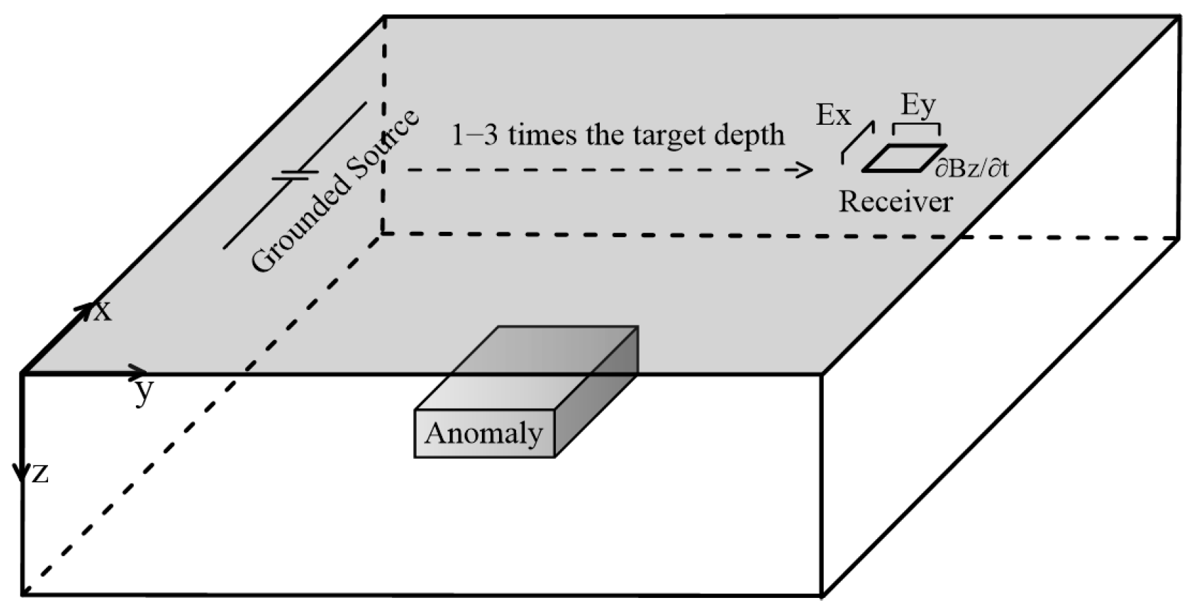
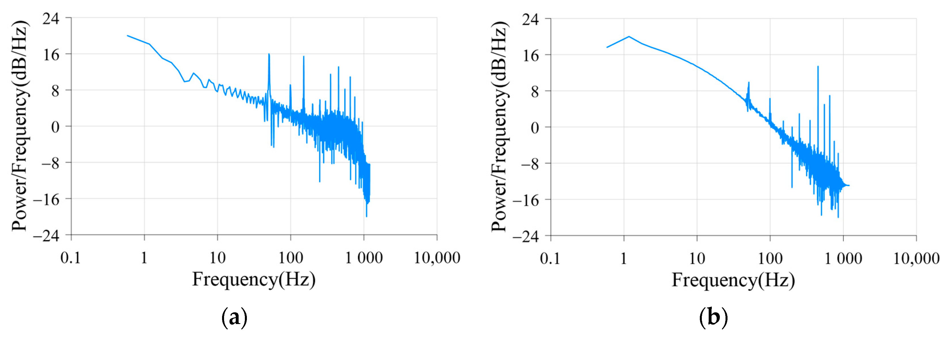
2. Analysis of LOTEM Signal Characteristics and Noise Sources

LOTEM is a method that uses 2–5 km long grounded wires to send a pulse primary electromagnetic field to the subsurface. The transmission waveform is a bipolar zero-crossing square wave (TD50) with a long time window (1-64S) and a duty cycle of 1:1. The offset distance of the transmitter and receiver is 1–3 times the detection depth (Figure 1). The secondary eddy current electromagnetic field is observed by coils and grounding electrodes in terms of spatial and temporal distribution. The strength and decay rate of the secondary field is closely related to the size, location, occurrence, and conductivity of the geological anomaly to be detected. LOTEM works in the time domain, observing pure secondary field with a wide frequency band. There is no interference from the primary field and high-power multi-pulse excitation. Repeated measurements and spatial domain multiple coverage technology can improve the signal-to-noise ratio. Compared with other methods such as MT and CSAMT, LOTEM has significantly higher resolution and exploration depth up to 3000–5000 m [24,25,26] and is sensitive to resistivity anomalies. It is widely used in underground mineral resources exploration, fluid identification of oil and gas reservoirs, hydraulic fracturing, and residual oil and gas dynamic monitoring [3,27,28,29,30,31].
Transient electromagnetic signals have a large dynamic range. Generally, the early signal has high amplitudes and fast decay rates, while the late signal has low energy and is easily overwhelmed by strong interfering noise signals. The early signal reflects the electrical properties of shallow subsurface media, while the late signal approaches zero with a relatively stable decay rate, reflecting the geoelectric characteristics of the bedrock. By contrast, the decay rate of the transient electromagnetic secondary field signal in a low-resistivity conductor is relatively slow, resulting in larger response values and longer decay times in the measurement. The opposite is true for high-resistivity conductors (Figure 2) [32].
The LOTEM-measured signal has dynamic, transient characteristics with many sources of interference. The signal often contains severe mixed interference and distortion (Figure 3). The noise sources mainly include natural and cultural interference, signal distortion caused by geological noise, and instrument noise. Natural electromagnetic interference signals are mainly Magnetotelluric (MT) source signals related to medium and high frequencies and lightning activity. Low frequencies manifest as ultra-long periodic changes associated with solar wind activity. Natural noise also includes wind noise, especially in the southern regions of China, where the climate is harsh. This type of interference is long-term and severe. Cultural interference is mainly related to human activities, including electromagnetic noise generated by power grids, mines, road traffic, industrial electricity, mobile communication networks, limited broadcasting, and radio stations.
Cultural interference is characterized by random, intermittent pulse signals and periodic fixed electromagnetic signals. Stable cultural interference is relatively easy to eliminate. However, interference caused by changes in the load that result in amplitude and phase distortion (such as saturation) is difficult to eliminate. In most parts of China, power grid overload is common due to power shortages. During overload, the time-domain characteristics of this type of signal appear as a sinusoidal wave that does not reach its peak and saturates. The waveform is similar to a trapezoidal wave. Therefore, the interference frequency is no longer a single harmonic but a wideband interference [33]. Geological noise is mainly caused by signal distortion caused by terrain and shallow subsurface electrical anomalies. It manifests as an overall shift of the signal. In addition, the existence of polarization can cause a negative overshoot in the observed signal (Figure 3) [34,35]. The influence of measurement and instrument systems mainly manifests as nonlinear interference and various drifts. The instrument is an electrical interference source with inherent electrical noise. This interference can be very strong if the instrument is too close to the coil. Electromagnetic coupling between the transmitter and receiver can also cause time-domain signal distortion.

3. LOTEM Denoising Process and Methods

3.1. Denoising Process

LOTEM reception signals include the primary field signal at the time of transmission, the mixed signal during the off period, and the pure secondary field signal induced after the off period. The primary field signal has strong and stable energy. After complete shutdown, the signal decays sharply and shows strong step characteristics overall (Figure 4). The signal has a large dynamic range. Known pre-stack time-domain filtering methods mainly include recursive filtering, median filtering, and power frequency interference window filtering, which often cause serious distortion of early signals of the secondary field decay [16,36,37], greatly reducing the confidence level of useful secondary field signals. By contrast, the power frequency and its harmonic interferences in the measured LOTEM signals show periodicity, but the main frequency fluctuates and oscillates within a limited range. As shown in Figure 5, this study designed 200 periodic signals with power frequency and its harmonic fluctuations, among which the bandwidth of the 50 Hz power frequency interference and its harmonics randomly varies within ±0.5 Hz, and the signal amplitude and phase randomly fluctuate within ±10%. When positive or negative signals are superimposed, an apparent periodic power frequency interference is exhibited, and this oscillating periodic signal is effectively weakened and eliminated by positive–negative superposition.
Given the characteristics of the LOTEM signal, it is proposed not to use time-domain filtering algorithms before signal stacking but to first stack signals and then use recursive filtering strategies (Figure 6), followed by inverse time-domain recursive filtering and windowed signal processing. Most random interference can be eliminated, and the interference of characteristic periodic signals can be weakened through periodic stacking and positive and negative stacking, and geological noise can also be effectively suppressed. Then, the inverse filtering algorithm is adopted to faithfully preserve the early-stage signals of the secondary decay and effectively suppress the periodic signals. Finally, high-quality secondary decay curves are obtained through stacking and windowing overlapping.

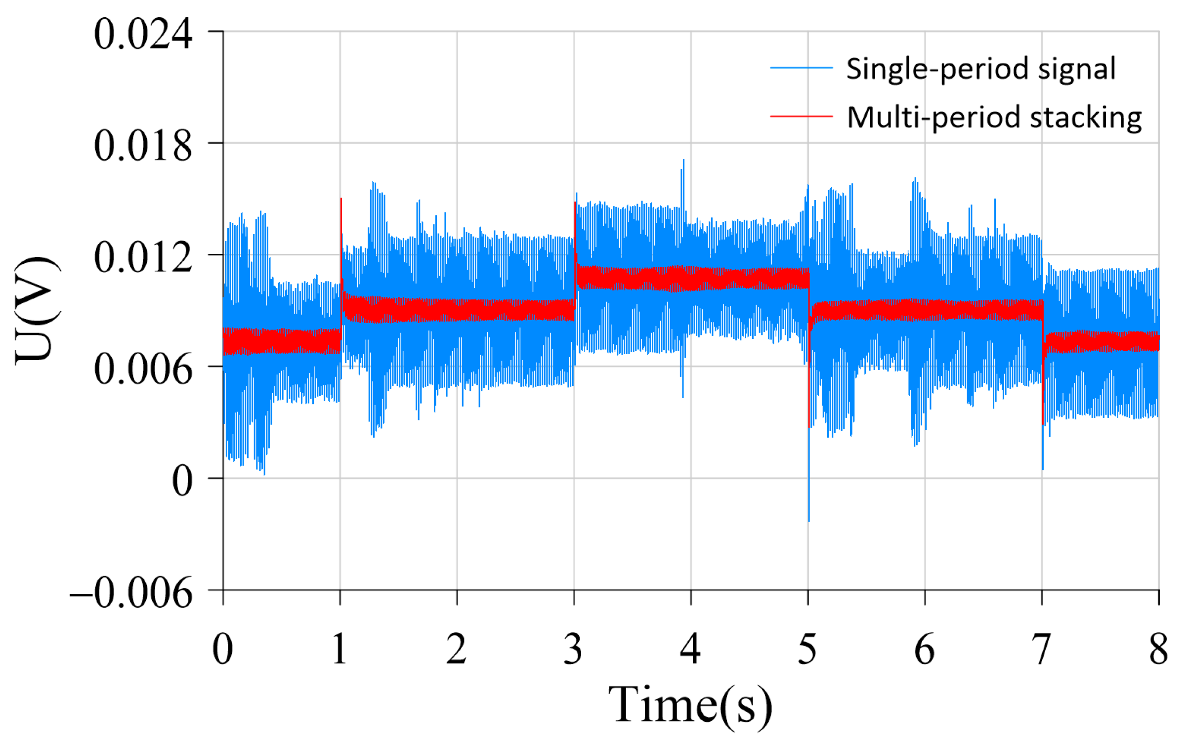
3.2. Signal Stacking

Natural sources (such as lightning activity) and various human interferences (e.g., factories, water pumps, electric fences, trains, vehicles) can all bring random noise. The amplitude of these noises is often much higher or much lower than the average signal level (high and low energy peaks). If these noises are superimposed on the received signal and cannot be well identified, they seriously impact the stacking effect.
LOTEM generally uses seismic-like multiple-stacking techniques to eliminate random and Direct Current (DC) interference. By continuously transmitting TD50 square waves multiple times, multiple time series of the same period are obtained. After human–machine interaction to screen out problematic and evident interference period sequences, full-period stacking and bipolar positive–negative stacking are performed to eliminate most random interference.
Expression for multi-period stacking is as follows:
S a l l t = i = 1 n S i t
S m e a n t = i = 1 n S i t n
In the above equation, S a l l t is the cumulative sum of all periods, S i t is a specific period among them, and S m e a n t is the output of the full-period stacking process (Figure 7).
Positive–negative stacking takes the time series collected by the negative excitation signal in the bipolar square wave and superimposes it with the positive time series after inversion. Finally, the waveform of half-period transmission shutdown can be obtained. The expression is as follows:
S t = S u p t + S d o w n t 2
where S u p t is the positive upward step time series, S d o w n t is the negative downward step time series, and S t is the output result of positive–negative stacking processing. The time series after two stackings can eliminate most random and drift interferences Figure 8).
Figure 7 shows that the multi-period stacking technology can effectively reduce random interference, especially for irregular and unpredictable interference. In addition, Figure 8 shows that the positive–negative stacking technology can eliminate random interference and directly weaken the effects of static and DC offset, thereby significantly improving signal quality. Furthermore, by comparing the power spectra before and after stacking in Figure 9, it can be seen that multi-period stacking and positive–negative stacking techniques can, to some extent, suppress fixed interference (such as 50 Hz and its harmonics). Therefore, multiple overlapping stacking processing techniques are a crucial measure to improve the quality of LOTEM data.

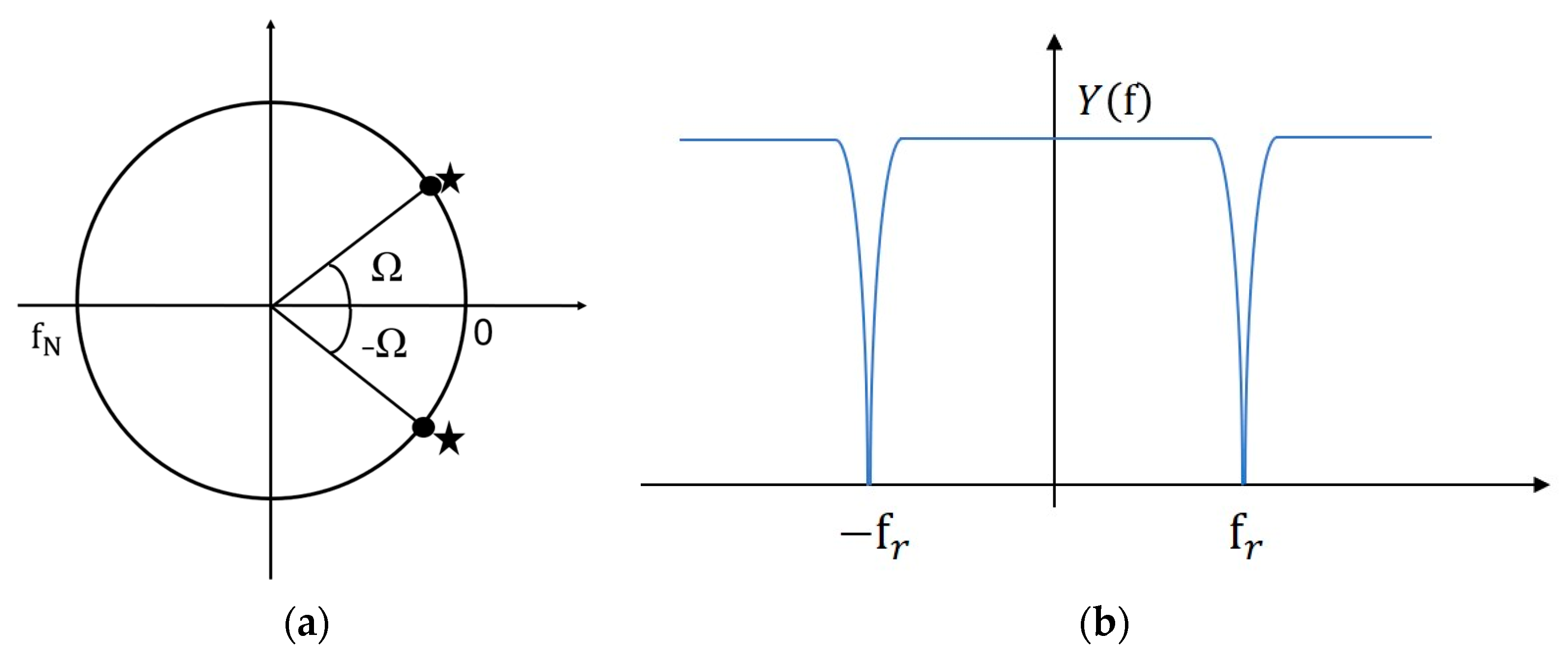
3.3. Time-Domain Inverse Digital Recursive Filter

Although the LOTEM method has high transmission power, deep exploration depth, strong anti-interference ability, and convenient flexibility, many measurement points still have a low signal-to-noise ratio due to cultural interference, and their data are often uninterpretable. To improve the quality of interpretation, “denoising” is the basic work in the early stage of electromagnetic data processing. Time-domain recursive filtering is a type of feedback filtering. It can improve the calculation speed of filtering, thus significantly saving time for the on-site processing of LOTEM data and improving work efficiency.

3.3.1. Concept of Recursive Filtering

Suppose the time series recorded during the LOTEM sampling period is x i , i = 1,2 , , N and the filter factor is h j , then the filtered time series y i is:
y i = j = + h j x i j
In practical calculations, the filter factor h j can only take a finite number of terms, which inevitably produces errors. To reduce errors, h j must be taken as a finite number of terms but with a large number of terms. This not only occupies a large amount of memory but also takes time. Recursive filtering can solve this problem well.
The idea of recursive filtering is to assume that the output values y i are related to each other. Therefore, when calculating y i , the previous calculation results y i 1 , y i 2 must be used. According to this idea, the conventional recursive filtering formula is:
y i = a 0 x i + a 1 x i 1 + + a n x i n b 1 y i 1 + b 2 y i 2 + + b m y i m
where m and n are natural numbers, and a n and b m are recursive filtering parameters.

3.3.2. Time-Domain Inverse Digital Filter Design Method

LOTEM measurement signals are often subject to interference at specific fixed frequencies, so the design of the filter should be a notch filter for a particular fixed frequency while keeping the rest of the spectrum unchanged [38]. The Z-plane method is a simple time-domain recursive notch filter [16,36,39], which selects appropriate zeros and poles on the Z-plane according to the requirements of the filter for amplitude and phase. According to the basic theory of Z-transform, the Z-transform of the amplitude–frequency characteristic of the filter described by Formula (5) can be written as:
W z = a 0 + a 1 z + + a n z n 1 + b 1 z + b 2 z 2 + + b m z m
The Z-plane method uses the notch characteristics of the amplitude–frequency function corresponding to the zero point on the unit circle and the pole near it (Figure 10) to quickly determine W z ; that is, the amplitude value at f r , f r should be 0. The amplitude value outside these two points is 1 (normalized value). To meet the above two conditions, it is required that the amplitude function must contain both zeros and poles, and the zeros and poles should be very close. For this reason, we can construct the frequency response of the filter based on Formula (5) as follows:
W z = G z z z z z z * z z p z z p *
Below we use the Z-plane method to quickly determine W z , and then use Formula (5) to conveniently write out the recursive expression of the time-domain recursive filter.
The complex form of zeros and poles in the Z-plane can be written as:
z z = cos Ω r ± sin Ω r = R z ± i I z
z p = r p cos Ω r ± r p sin Ω r = R p ± i I p
where Ω r is the angular frequency to be notched, and its mathematical expression is:
Ω r = ± 180 ° · f r / f N
where f r is the frequency to be notched, f N is the Nyquist frequency, according to the sampling theorem:
f N = 1 / 2 t
Substituting Formulas (8) and (9) into Formula (7) and through simple mathematical operations, the frequency response of the notch filter can be written as:
W z = G z 2 2 R z z + R z 2 + I z 2 1 + 2 R p z + z 2 / R p 2 + I p 2
G is obtained by setting W z = 1 when Nyquist frequency f N = π , that is:
G = 1 + 2 R p + 1 / R p 2 + I p 2 / 2 + 2 R z
According to Formulas (5), (6) and (12), we can conveniently write out the mathematical expression of the time-domain recursive filter:
y n = G R z 2 + I z 2 x n 2 G R z x n 1 + G x n 2 1 / R p 2 + I p 2 y n 2 + 2 R p / R p 2 + I p 2 y n 1
However, two points should be noted when processing recursive filtering. First, it is necessary to accurately grasp the main frequency of interference signals to avoid distortion of useful signals caused by filtering processing. Second, attention should be paid to the Gibbs effect of the filter; that is, oscillation may occur at signal endpoints after filtering. To ensure that the accuracy of early signals is not compromised, it is necessary first to inverse the signal and then filter it (filtering from back to front). Although there is some oscillation in late signals after filtering, it does not substantially impact the signal since its duration far exceeds what is needed. As shown in Figure 11, forward filtering (blue) undergoes a violent jump in gradient in the early signal period, resulting in severe signal distortion. At the same time, inverse filtering (red) well preserves signal data with only a small amount of oscillation on late signals that are not too concerned.

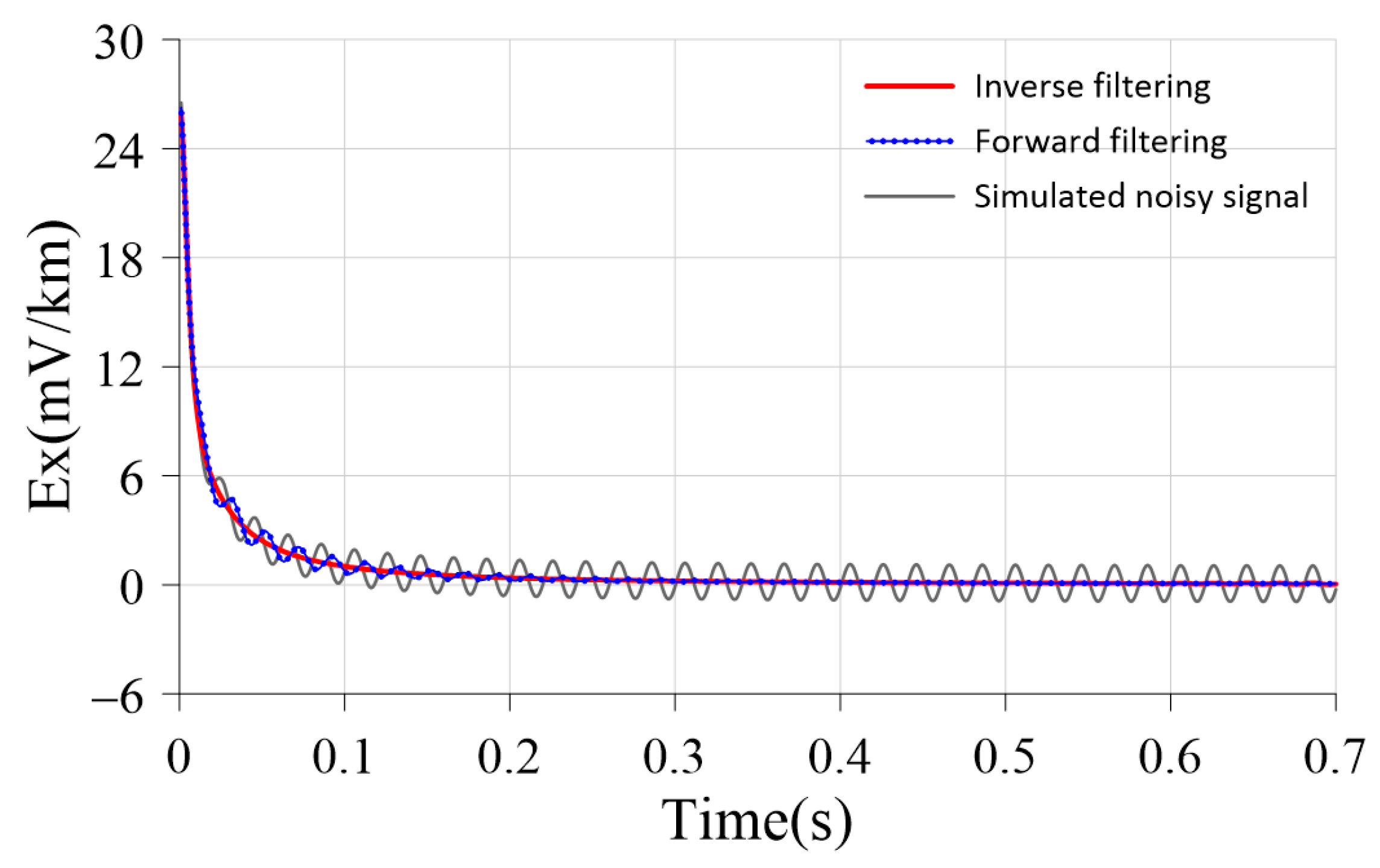
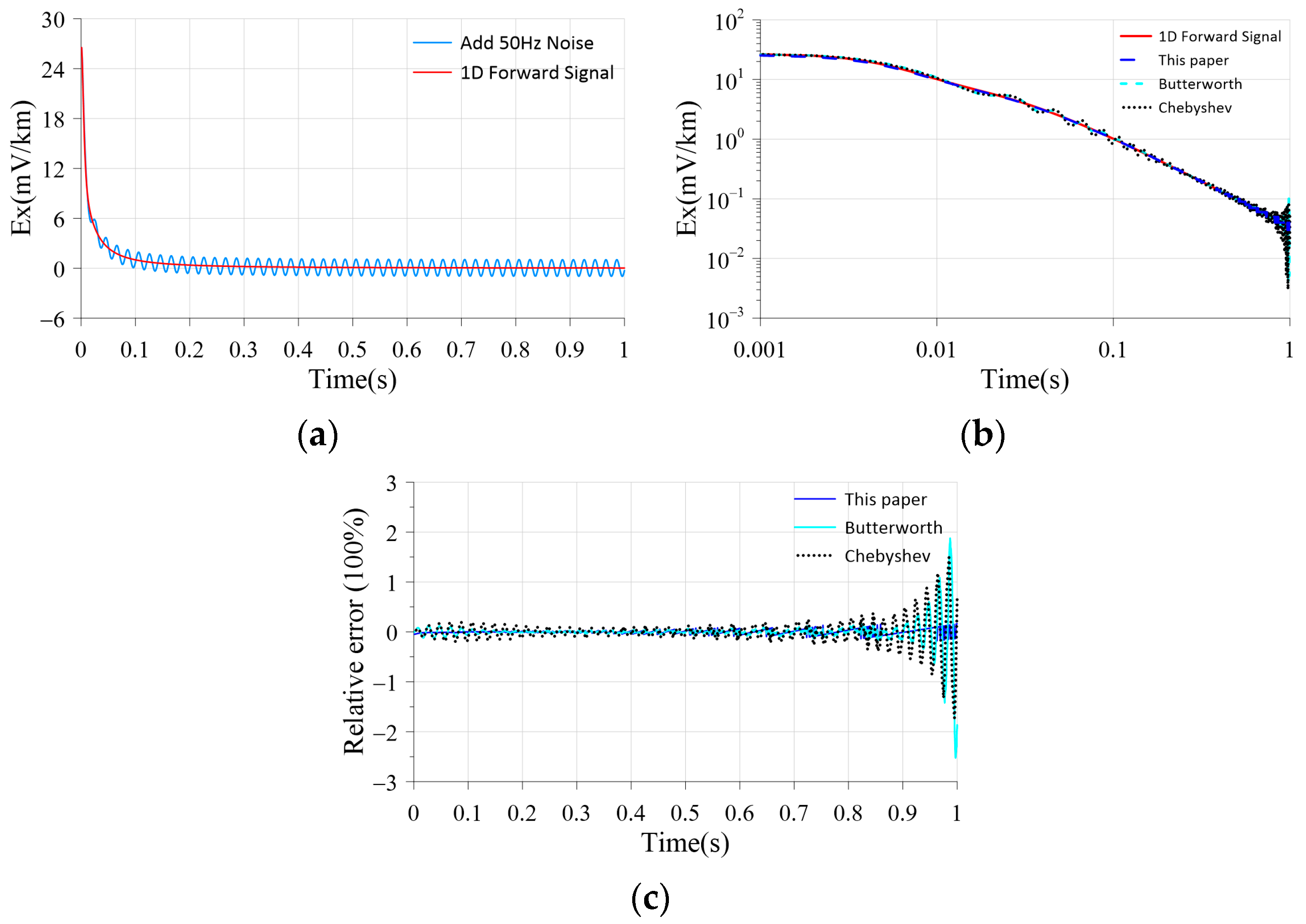
3.4. Algorithm Verification

To test the effectiveness of the filtering method proposed in this paper, we calculated the theoretical LOTEM response signal using a forward algorithm and added 50 Hz periodic noise with a signal-to-noise ratio of 10 dB to form a test signal. The original and noise-added induced electromotive force attenuation curves are shown in Figure 12a. Time-domain inverse digital filtering, Butterworth band-stop filter, and Chebyshev band-stop filter were used to filter the noise-added curve, and the original and filtered induced electromotive force attenuation curves are shown in Figure 12b. It can be seen that the method proposed in this paper has a good filtering effect on the noise-added attenuation curve, basically restoring the original curve shape of the measured data and suppressing most of the noise, which is significantly better than the other two methods. By calculating the relative errors of the three methods (Figure 12c), it can be seen that the relative error of the method proposed in this paper is smaller than that of the other two methods at all times, especially in the late signal part.
In addition, this paper quantitatively estimates the effectiveness of denoising methods through Root Mean Squared Error ( R M S E ) [40] or the size of Signal-to-Noise Ratio ( S N R ) [41] before and after filtering. R M S E and S N R are defined as:
R M S E = i = 1 n d i 2 / N
S N R = 10 × log 10 s i g P o w e r / n o i s e P o w e r
where N is the number of samples, d i is the difference between the filtered curve and the forward modeling standard curve, s i g P o w e r is the signal power, and n o i s e P o w e r is the noise power. The smaller the value of R M S E , the higher the similarity between the two signals; the larger the signal-to-noise ratio, the better the denoising effect. Table 1 shows the root mean square error and signal-to-noise ratio of the simulated noisy signal and three different filtered denoised signals. It can be seen that the algorithm proposed in this paper effectively reduces the R M S E value and improves the S N R value after denoising. The denoised signal has a high degree of overlap with the theoretical signal and a small error.

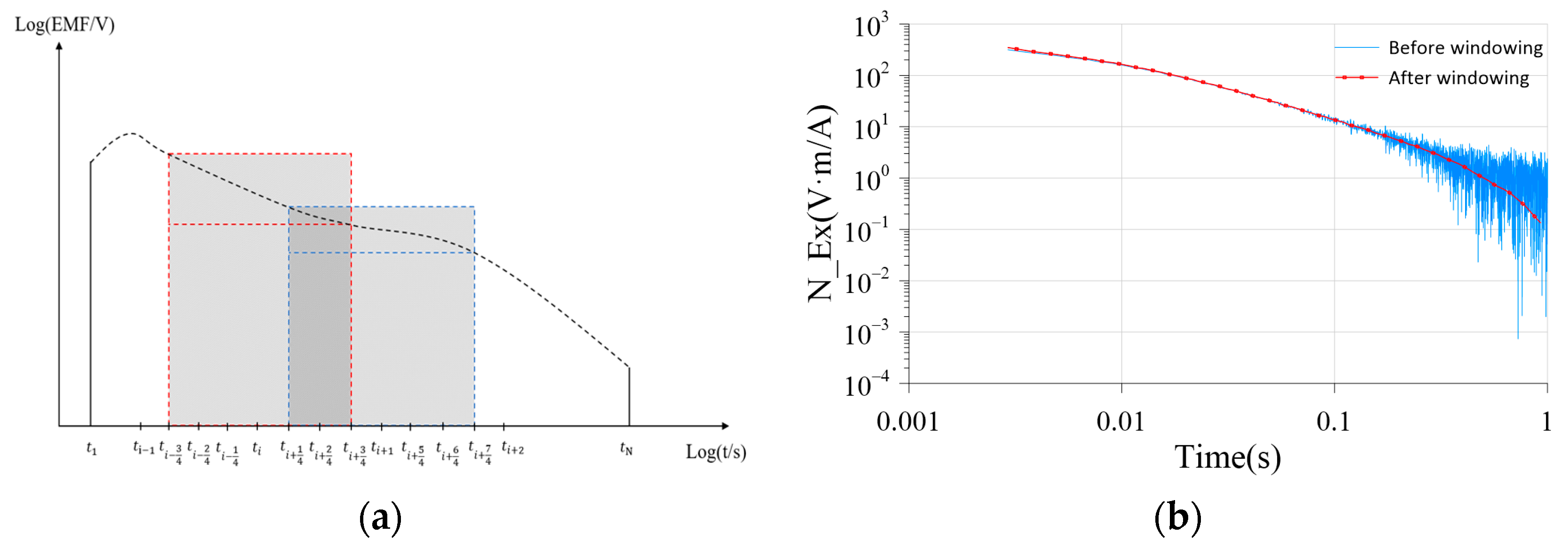
3.5. Window Smoothing

After stacking processing and recursive filtering, window processing is also required. Windowing aims to eliminate spike interference and ensure the curve is continuous and smooth. Generally, the median filtering method is used for windowing, and overlapping technology is selected according to the size of the window (Figure 13a). The overlapping ratio can be adjusted according to actual needs with an adjustment range of 10%–50%. Figure 13b shows the comparison effect before and after window smoothing. It can be clearly seen that after windowing, the curve is very smooth and well preserves the attenuation trend.

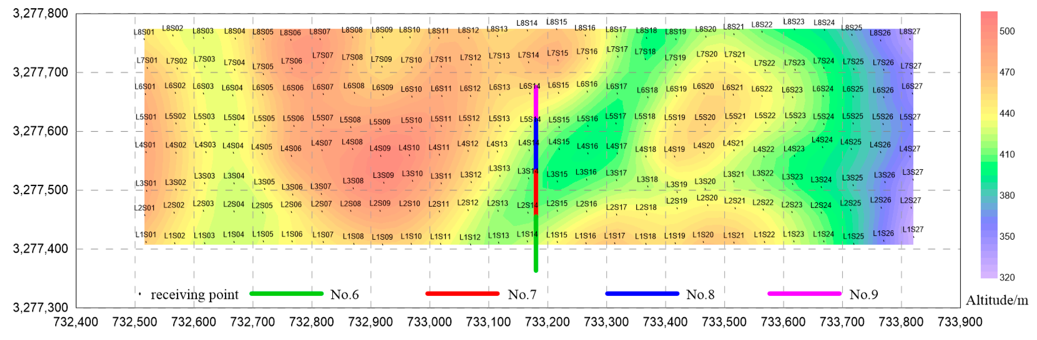
4. Analysis of the Processing Effect of Measured Data

The hydraulic fracturing LOTEM method dynamic monitoring test area is located in Fuling District, Chongqing City, adjacent to Wujiang River in the north, with convenient transportation and low mountains and hills as the main terrain [42]. The experiment laid out eight survey lines covering the 7th–9th fracturing sections of the horizontal well (Figure 14). Each survey line was 1350 m long with an electrode spacing of 50 m and a total of 216 physical points (Figure 15). The transmission pole distance AB was 4000 m, and the offset distance was 5000 m. A 200-kW high-power transmission system was used. The transmission waveform was a bipolar zero-crossing square wave (TD50) with a duty cycle 1:1 and a period of 8 s. The current size was 48 A. The DRU electromagnetic acquisition system developed by the Institute of Geology and Geophysics, Chinese Academy of Sciences [43,44,45] was used with a sampling rate of 2400 Hz.
Figure 16a shows the field-measured data, and Figure 16b presents the corresponding spectrum. The survey area has strong power frequency and random impulse interference, resulting in an extremely low signal-to-noise ratio of the original data. After selecting all single-period data through human–computer interaction, the signal was subjected to period stacking (as shown in Figure 17), effectively reducing random impulse interference and visibly reducing the “spikes” on the curve. Then, positive and negative polarity stacking was applied to the period-stacked data (Figure 18), further smoothing the curve convergence. However, strong 50 Hz and its harmonic interference could still be found in the half-period curve and its spectrum. After filtering (Figure 19) and window smoothing (Figure 20) with the method proposed in this paper, the curve became exceptionally smooth, restoring the measured attenuation curve under the no-interference situation and making the previously blurred trend clear and visible. The corresponding spectrum also demonstrated that 50 Hz and its harmonics were significantly suppressed (Figure 19b).
Additionally, we applied the denoising process to transient electromagnetic data from a copper–iron metal mine in Daye City, Hubei Province. The test area is located 1 km southwest of Daye City in the Tonglushan mining area in southeastern Hubei. High-speed and national highways pass through the mining area from east to west, and the area is rich in cultural facilities and contains high-intensity power frequency interference (Figure 21b). Under strong power frequency interference, the electromagnetic field signal is completely masked, and it is difficult to identify the presence of the signal from the curve (Figure 21a).
In Figure 22a, the red line represents the signal obtained after processing with the stacking-filtering-window smoothing mode proposed in this paper. It can be seen that this signal has no periodic noise, and the signal shape is clearly visible. From its corresponding spectral curve, it can be seen that the sharp peaks of 50 Hz and its harmonic interference are well suppressed (Figure 22b).
The comparison of time series and spectra of measured data from Fuling shale gas and Daye copper–iron metal mine fully demonstrates that the method proposed in this paper can effectively suppress various mixed noise interference in field-measured data. It is a practical and effective denoising method for long-offset transient electromagnetic data.

5. Conclusions

This paper proposes a systematic noise interference suppression process and method by deeply analyzing the characteristics of LOTEM signals and their noise sources. First, multi-period and positive–negative bipolar signal stackings were used to remove random noise and suppress DC offset signals. Then, the time-domain inverse digital recursive method was applied to remove characteristic frequency signals, such as industrial frequency signals and their harmonic interference. Finally, high-quality transient electromagnetic secondary field attenuation signals were obtained through overlapping windowing technology.
Based on the one-dimensional layered model, theoretical time-domain response data simulation was performed, and MATLAB was used to add simulated 50 Hz sine wave interference. Finally, filtering and denoising were performed on the noisy data. Compared with before processing, the Signal-to-Noise Ratio (SNR) of the simulated signal after processing with the filtering method proposed in this paper was significantly improved, and the Root Mean Squared Error (RMSE) was significantly reduced. This method was applied to processing time-domain electromagnetic data for dynamic monitoring of hydraulic fracturing in the Fuling shale gas and Daye copper–iron metal mine. The signal waveform and spectrum before and after processing were compared. The results show that the method proposed in this paper suppresses various electromagnetic noises in long-offset transient electromagnetic exploration, improves data quality, and is an effective time-domain long-offset transient electromagnetic data denoising method.

Author Contributions

Conceptualization, Y.X. and X.X.; methodology, Y.X. and X.X.; validation, B.X.; resources X.X., L.Z. and L.Y.; writing—original draft preparation, Y.X.; writing—review and editing, X.X. and L.Z.; supervision, L.Y. All authors have read and agreed to the published version of the manuscript.

Funding

This research was funded by the National Natural Science Foundation of China, grant number 42274103; the National Natural Science Foundation of Key Project of China, grant number 42030805; and the Science and Technology Department Project of China Petroleum & Chemical Corporation, grant number P22163.

Data Availability Statement

The datasets used and/or analyzed during the current study are available from the corresponding author upon reasonable request.

Conflicts of Interest

The authors declare that they have no known competing financial interests or personal relationships that could have appeared to influence the work reported in this paper.

References

  1. Strack, K. Exploration with Deep Transient Electromagnetics; Elsevier: Amsterdam, The Netherlands, 1992; ISBN 978-0444895417. [Google Scholar]
  2. Keller, G.V. Electromagnetic Surveys in the Central Volcanic Region; Geophysics Division Report; Geophysics Division: Wellington, New Zealand, 1969. [Google Scholar]
  3. Kaufman, A.A.; Keller, G.V. Frequency and Transient Soundings; Elsevier: Amsterdam, The Netherlands, 1983; Volume 55, p. 65. [Google Scholar]
  4. Newman, G.A. Deep transient electromagnetic soundings with a grounded source over near-surface conductors. Geophys. J. Int. 1989, 98, 587–601. [Google Scholar] [CrossRef]
  5. Commer, M.; Helwig, S.L.; Hördt, A.; Scholl, C.; Tezkan, B. New results on the resistivity structure of Merapi Volcano (Indonesia), derived from three-dimensional restricted inversion of long-offset transient electromagnetic data. Geophys. J. Int. 2006, 167, 1172–1187. [Google Scholar] [CrossRef]
  6. Vozoff, K.; Moss, D.; LeBrocq, K.; McAllister, K. LOTEM electric field measurements for mapping resistive horizons in petroleum exploration. Explor. Geophys. 1985, 16, 309–312. [Google Scholar] [CrossRef]
  7. Piao, H.R. Principles of Electromagnetic Sounding; Geological Publishing House: Beijing, China, 1990. [Google Scholar]
  8. Xue, G.Q.; Li, X.; Di, Q.Y. The progress of TEM in theory and application. Prog. Geophys. 2007, 22, 1195–1200. [Google Scholar]
  9. Macnae, J.; Lamontagne, Y.; West, G. Noise processing techniques for time-domain EM systems. Geophysics 1984, 49, 934–948. [Google Scholar] [CrossRef]
  10. Andrew, K.H. Application of frequency-domain polyphase filtering to quadrature sampling. Proc. Spie 1995, 2563, 450–457. [Google Scholar]
  11. An, H.B.; Shen, Y.Y. A method to suppress narrow-band interference based on frequency domain filter. Optoelectron. Technol. Inf. 2004, 18, 64–68. [Google Scholar]
  12. Cui, Z.; Cheng, M.; Wu, Q.; Wang, B. A technique of fast median filtering and its application to data quality control of doppler radar. Plateau Meteorol. 2005, 24, 727–733. [Google Scholar]
  13. Mörbe, W.; Yogeshwar, P.; Tezkan, B.; Hanstein, T. Deep exploration using long-offset transient electromagnetics: Interpretation of field data in time and frequency domain. Geophys. Prospect. 2020, 68, 1980–1998. [Google Scholar] [CrossRef]
  14. Bai, F.F.; Miao, C.Y.; Zhang, C.; Gan, J.M. Studying on denoising algorithm of heart sound signal based on the generalized mathematical morphology. In Proceedings of the IEEE 10th International Conference on Signal Processing Proceedings, Beijing, China, 24–28 October 2010; pp. 1797–1800. [Google Scholar]
  15. Zhou, Y.X. Research and Application of Adaptive Filtering in Transient Electromagnetic Denoising. Master’s Thesis, Chengdu University of Technology, Chengdu, China, 2018. [Google Scholar]
  16. Strack, K.; Hanstein, T.; Eilenz, H. LOTEM data processing for areas with high cultural noise levels. Phys. Earth Planet. Inter. 1989, 53, 261–269. [Google Scholar] [CrossRef]
  17. Li, S.Y.; Lin, J.; Yang, G.H.; Tian, P.P.; Wang, Y.; Yu, S.B.; Ji, Y.J. Ground-Airborne electromagnetic signals de-nosing using a combined wavelet transform algorithm. Chin. J. Geophys. 2013, 56, 3145–3152. (In Chinese) [Google Scholar]
  18. Liu, J.; Lei, W.; Zhang, Y.; Yang, W. The Application Research of TEM De-noising Based on Improved Wavelet Threshold Function. Chin. J. Eng. Geophys. 2014, 11, 547–552. [Google Scholar]
  19. Zhao, J.P.; Huang, D.J. Mirror extending and circular spline function for empirical mode decomposition method. J. Zhejiang Univ.-Sci. A 2001, 2, 247–252. [Google Scholar] [CrossRef]
  20. Julian, L.G.; Danilo, R. A simple method inspired by empirical mode decomposition for denosing seismic data. Geophysics 2016, 81, 403–413. [Google Scholar]
  21. Han, J.J.; Banan, M.V.D. Empirical mode decomposition for seismic time-frequency analysis. Geophysics 2013, 78, 9–19. [Google Scholar] [CrossRef]
  22. Li, C.W.; Dong, L.H.; Wang, Q.F.; Wang, F.Y.; Hu, B.; Xu, X.M. Noise auto identification and de-noising method of coal-rock weak electromagnetic signals. J. China Coal Soc. 2016, 41, 1933–1940. [Google Scholar]
  23. Wu, S.H.; Huang, Q.H.; Zhao, L. De-noising of transient electromagnetic data based on the long short-term memory-autoencoder. Geophys. J. Int. 2020, 224, 669–681. [Google Scholar] [CrossRef]
  24. Caldwell, T.G.; Bibby, H.M. The instantaneous apparent resistivity tensor: A visualization scheme for LOTEM electric field measurements. Geophys. J. Int. 1998, 135, 817–834. [Google Scholar] [CrossRef]
  25. Ziolkowski, A.; Hobbs, B.A.; Wright, D. Multitransient electromagnetic demonstration survey in France. Geophysics 2007, 72, F197–F209. [Google Scholar] [CrossRef]
  26. Haroon, A.; Adrian, J.; Bergers, R.; Gurk, M.; Tezkan, B.; Mam Madov, A.; Novruzov, A. Joint inversion of long-offset and central-loop transient electromagnetic data: Application to a mud volcano exploration in Perekishkul, Azerbaijan. Geophys. Prospect. 2015, 63, 478–494. [Google Scholar] [CrossRef]
  27. Strack, K.M. Future Directions of Electromagnetic Methods for Hydrocarbon Applications. Surv. Geophys. 2014, 35, 157–177. [Google Scholar] [CrossRef]
  28. Airo, M.L. Geophysical signatures of mineral deposit types in finland. Geol. Surv. Finl. 2015, 58, 9–70. [Google Scholar]
  29. Spagnoli, G.; Hannington, M.; Bairlein, K.; Hördt, A.; Jegen, M.; Petersen, S.; Laurila, T. Electrical properties of seafloor massive sulfides. Geo-Mar. Lett. 2016, 36, 235–245. [Google Scholar] [CrossRef]
  30. Streich, R. Controlled-Source Electromagnetic Approaches for Hydrocarbon Exploration and Monitoring on Land. Surv. Geophys. 2016, 37, 47–80. [Google Scholar] [CrossRef]
  31. Xie, X.B.; Zhou, L.; Yan, L.J.; Hu, W.B. Remaining oil detection with time-lapse long offset & window transient electromagnetic sounding. Oil Geophys. Prospect. 2016, 51, 605–612. [Google Scholar]
  32. Yogeshwar, P. Resistivity-Depth Model of the Central Azraq Basin Area, Jordan: 2D Forward and Inverse Modeling of Time Domain Electromagnetic Data. Ph.D. Thesis, Universität zu Köln, Cologne, Germany, 2014. [Google Scholar]
  33. Yan, L.J. Electromagnetic Exploration Methods and Their Applications in Southern Carbonate Rock Regions; Petroleum Industry Press: Beijing, China, 2001. [Google Scholar]
  34. Spies, B.R. A filed occurrence of sign reversals with the transient electromagnetic method. Geophys. Prospect. 1980, 28, 620–633. [Google Scholar] [CrossRef]
  35. Lee, T. Transient electromagnetic response of a polarizable ground. Geophysics 1981, 46, 1037–1041. [Google Scholar] [CrossRef]
  36. Shanks, J. Recursion filters for digital processing. Geophysics 1967, 32, 33–51. [Google Scholar] [CrossRef]
  37. Kulhanek, O. Introduction to Digital Filtering in Geophysics; Elsevier: Amsterdam, The Netherlands, 1976. [Google Scholar]
  38. Claerbout, J.F. Fundamentals of Geophysical Data Processing with Applications to Petroleum Prospecting; Blackwell Science Inc.: Oxford, UK, 1985; ISBN 978-0865423053. [Google Scholar]
  39. Li, B.F. Data processing of Geophysical prospecting. J. Ocean. Univ. Qingdao 1994, S3, 144–147. [Google Scholar]
  40. Zhang, C.G. Application of Wavelet Analysis in Signal Denoising. Master’s Thesis, University of Electronic Science and Technology, Chengdu, China, 2018. [Google Scholar]
  41. Zhong, J.J.; Song, J.; You, C.X.; Yin, X.Q. Wavelet de-noising method with threshold selection rules based on SNR evaluations. J. Tsinghua Univ. Sci. Technol. 2014, 54, 259–263. (In Chinese) [Google Scholar]
  42. Di, Q.Y. New Technologies and Applications of Electromagnetic Detection in Major Geological Engineering Projects; Science Press: Beijing, China, 2020; ISBN 9787030671011. [Google Scholar]
  43. Di, Q.Y.; Fang, G.Y.; Zhang, Y.M. Research of the Surface Electromagnetic Prospecting (SEP) system. Chin. J. Geophys. 2013, 56, 3629–3639. (In Chinese) [Google Scholar]
  44. Di, Q.Y.; Xue, G.Q.; Wang, Z.X.; He, L.F.; Pei, R.Z.; Zhang, T.X.; Fang, G.Y. Lithospheric structures across the Qiman Tagh and western Qaidam Basin revealed by magnetotelluric data collected using a self-developed SEP system. Sci. China Earth Sci. 2021, 64, 1813–1820. [Google Scholar] [CrossRef]
  45. Di, Q.Y.; Fu, C.M.; An, Z.G.; Xu, C.; Wang, Y.L.; Wang, Z.X. Field testing of the surface electromagnetic prospecting system. Appl. Geophys. 2017, 14, 449–458. [Google Scholar] [CrossRef]
Figure 1. Schematic diagram of the LOTEM working principle.
Minerals 13 01084 g001
Figure 2. (a) Waveform of the transmitted pulse; (b) the response characteristics of the secondary field for different resistivities (Reproduced with permission from [32] (Figure 2.2 therein)).
Minerals 13 01084 g002
Figure 3. Various interference waveforms in the experimental area. (a) Pulse noise; (b) DC offset; (c) random noise; (d) periodic noise.
Minerals 13 01084 g003
Figure 4. (a) LOTEM measured signal; (b) its frequency spectrum.
Minerals 13 01084 g004
Figure 5. Verification of stacking. (ac) Respectively, represent the down-ward step signal, multi-period signal stackings, and its spectrum; (df) respectively, represent the upward step signal, multi-period signal stackings, and its spectrum; (g,h) respectively, represent positive–negative bipolar signal stackings and its spectrum.
Minerals 13 01084 g005
Figure 6. Flowchart of the denoising process.
Minerals 13 01084 g006
Figure 7. Waveform of multi-period stacking.
Minerals 13 01084 g007
Figure 8. Waveform of positive–negative stacking.
Minerals 13 01084 g008
Figure 9. (a) Frequency spectrum before stacking; (b) frequency spectrum after stacking.
Minerals 13 01084 g009
Figure 10. (a) Distribution of zeros and poles in the Z-plane; (b) amplitude–frequency characteristics of the notch filter.
Minerals 13 01084 g010
Figure 11. Schematic diagram of forward and inverse filtering comparison.
Minerals 13 01084 g011
Figure 12. (a) Forward modeling and noise comparison; (b) filtering verification of three filtering methods; (c) the relative error of three filtering methods.
Minerals 13 01084 g012
Figure 13. (a) Overlapping window; (b) window effect diagram.
Minerals 13 01084 g013
Figure 14. Field deployment diagram of transmission and reception points.
Minerals 13 01084 g014
Figure 15. Distribution map of the measurement points.
Minerals 13 01084 g015
Figure 16. (a) Field-measured data; (b) its spectrum.
Minerals 13 01084 g016
Figure 17. Multi-period stacking effect diagram.
Minerals 13 01084 g017
Figure 18. (a) Positive and negative bipolar stacking; (b) its spectrum.
Minerals 13 01084 g018
Figure 19. (a) Filtering effect diagram; (b) its spectrum.
Minerals 13 01084 g019
Figure 20. Window smoothing effect diagram.
Minerals 13 01084 g020
Figure 21. (a) Measured data from the mining area; (b) its spectrum.
Minerals 13 01084 g021
Figure 22. (a) Waveform of measured data from the mining area after processing; (b) its spectrum.
Minerals 13 01084 g022
Table 1. Comparison of RMSE and SNR before and after signal filtering and denoising.
SignalRMSESNR
simulated noisy signal7.0715 × 10−710.1770
This paper7.8753 × 10−828.6625
Butterworth1.1810 × 10−725.3241
Chebyshev1.1703 × 10−725.3530
Disclaimer/Publisher’s Note: The statements, opinions and data contained in all publications are solely those of the individual author(s) and contributor(s) and not of MDPI and/or the editor(s). MDPI and/or the editor(s) disclaim responsibility for any injury to people or property resulting from any ideas, methods, instructions or products referred to in the content.

