Coal Mine Goaf Interpretation: Survey, Passive Electromagnetic Methods and Case Study

Abstract

Coal mine goaf detection remains confronted with the lack of fast, effective and low-cost exploration means, especially for the accurate prediction of mining threats primarily caused by hydraulic infiltration. The rapid popularization of passive electromagnetic methods has contributed greatly to improving the interpretation effects of different types of goafs. This paper, firstly, summarizes the pros and cons of various exploration methods in goaf detection. Then, the feasibility of goaf detection using novel passive electromagnetic methods (e.g., the super low frequency alternating magnetic component method (SLF) and audio frequency magnetotelluric method (AMT)) is proposed and further discussed. With well-designed geo-electrical goaf models, the theoretical results demonstrate that the semi-quantitative interpretation of SLF responses can be directly used for the delineation of the target layer in the estimated depth range. In contrast, 3D inversion provides more information about conductive targets with the appropriate initial model selection. Then, shallow, low-resistive targets can be more accurately allocated in the inversion maps. Moreover, the real data interpretation results from study areas demonstrate that the SLF method can utilize the magnetic component responses to effectively identify the fault structures, and indirectly contributes to judge the goaf collapse locations in favor of describing the potential distribution of fracture water infiltration. Combined with the three-dimensional (3D) resistivity inversion of AMT data, the low-resistive water-rich areas within the depth of 400 m were revealed. The inverted depth distributions are basically consistent with those of the water-filled goafs and surrounding layers, which were also confirmed by known logging data. The detailed delineations of water-control fracture zones can be inferred to relate to aquifers in some mining areas; this can reveal potential collapses that require successive mining planning. In specific working faces, goaf risks have been handled in advance by strengthening the continuous monitoring of the water level and water inflow. The above verification has laid a theoretical and practical foundation for passive electromagnetic interpretation methods for effectively predicting collapse-type risks or hydraulic threats in coal mine goafs.

1. Introduction

In recent years, the increasing demand for coal resources in sustainable production has become one of the most important topics all over the world. However, pervasive water-collapse disasters, a form of mine accident which has not been effectively prevented, occur frequently, especially in coal mine goafs [1]. Goafs, roof floors, collapse columns and other potential aquifers are the main factors in coal mining disasters [2,3]. Therefore, it is necessary to comprehensively evaluate the characteristics of different geophysical methods and select appropriate detection methods according to the geological settings and buried depths of goaf targets [3,4]. At present, almost all traditional exploration methods, including seismic methods, gravity, logging, radiation and electromagnetic methods, have been applied in goaf interpretation, combined with drilling [5], drainage and production data, temperature changes or thermal anomalies [6]. Seismic methods, including the shallow seismic reflection method, scattered or diffraction wave method, surface wave method (or microseismic method), tomography technology, etc., are mainly built on the wave velocity and impedance differences between goafs and surrounding roof-floor rocks, if coal seams are mined with the goafs formed [7,8]. It is widely acknowledged that complete coal seams possess low density and low velocity, with strong reflection waves and stable seismic events. In contrast, mine goafs could lead to damaged strata, which accounts for a strong attenuation effect, with distorted or misplaced events, on the seismic reflection waves [9]. This effect is characterized by irregular or even disordered reflection wave deformations [10,11]. The aforementioned reflection methods are inapplicable when the width of a goaf is less than its lateral resolution; thus, the diffraction method, the Rayleigh method and the microtremor seismic method (SMS) are introduced [8]. In addition, seismic velocity tomography can be obtained by the joint interpretation of the travel time, amplitude and signal frequency, and pressure inversion can also be carried out [12]. In particular, the extraction and application of seismic attributes can greatly improve detection results with high signal-to-noise ratio seismic data [13]. The radioactive method is also applied because of high radon concentration anomalies in coal mine goafs or collapse areas. As radon elements migrate to the surface through the caving fracture zone in a goaf, the locations of the coal mine goaf can be accurately delineated. However, it is difficult to determine goaf depth [14]. Additionally, the vertical density changes of the collapses in the goaf zones account for negative gravity anomalies, and the gravity method is characterized by three-dimensional apparent density inversion and the boundary identification of gravity anomalies [15,16]. Meanwhile, electromagnetic methods, based on electrical differences in the properties between goafs and surrounding rocks, such as resistivity, polarization parameters and electromagnetic absorption parameters, have also been employed [17,18,19]. The high-density resistivity method is used to analyze water-rich goafs [20]. The dipole–dipole device is suitable for a goaf with an exploration depth [21]. Transient electromagnetic method is also mainly aimed at a water-filled low-resistive goaf, and the changes of horizontal component responses are more sensitive than those of vertical component responses [22,23,24]. For a shallow goaf, a general central loop source device can be used. A large fixed source loop device possesses the advantages of high efficiency and high resolution [25]. Additionally, the dual-frequency induced polarization (IP) method was introduced because IP and amplitude frequency characteristics are reduced if a goaf forms [26]. Due to goaf deformation, synthetic aperture radar interferometry (InSAR) is used to obtain cumulative settlement in a continuous time [27], in addition to the deformation rate and surface deformation of goafs [28,29]. All exploration methods are summarized in detail in Table 1.

The current coal mine goaf interpretation technology was developed in the following directions: the joint method, from “the half space”, or from “the whole space” [30,31]. However, the widespread adoption of these methods remains limited because of the complex technology, high cost and low exploration efficiency involved. Therefore, a fast and efficient natural source method, i.e., the passive electromagnetic method, is rapidly being developed and applied. This method is based on the electromagnetic induction principle using the natural source’s electromagnetic observation data to produce an image of the electrical structure of the subsurface medium. The classical passive methods, such as geomagnetic sounding (GDS) and magnetotelluric sounding (MT), have entered full development [32]. In order to effectively analyze the theoretical electromagnetic responses of underground media, the equations mentioned in the following sections can be obtained on the assumptions of one-dimensional, two-dimensional and three-dimensional geoelectric models. Commonly used numerical simulation methods mainly include the finite difference method, finite element method and integral equation method, which lay a foundation for subsequent inversion [33]. The measured data is further fitted with the responses of the theoretical models after the signal spectrum estimation [34]. Regularization constraints are introduced to reduce the multiplicity of inversion solutions [35]; this multiplicity has gradually changed from one-dimensional and two-dimensional inversion to three-dimensional inversion [36]. Nowadays, the audio-frequency magnetotelluric method (AMT) has attracted greater attention because of its fast and economical exploration to a depth of less than 1000 m [37]. Predecessors used EH4 detection equipment (one popular AMT module) to preliminarily detect coal mine goafs [38] and to analyze water-rich distribution [39]. Additionally, passive electromagnetic component methods were applied [40]. To date, AMT inversion used for the effective interpretation of coal mine goafs has still not been explored and resolved. Passive electromagnetic methods mainly use the ratio of electric field and magnetic field components to obtain the impedances or magnetic ratio responses for resistivity inversion [41]. Although impedance calculation eliminates random fluctuation and time variation factors, it may weaken detailed changes, contained in electromagnetic components, related to underground structures [40,42]. In fact, natural source electric and magnetic components both contain detailed subsurface information [43].

In this paper, the potential advantages of passive electromagnetic methods in coal mine goaf interpretation will be systematically explored. Among them, semi-quantitative SLF inversion in collapse-type mining goaf areas will be discussed and validated. The stable 3D AMT inversion method is also proposed and examined by analyzing single-target and multi-target model results combined with types of initial models or data error bars. Preliminary field surveys could be subsequently accomplished using proposed electromagnetic methods with promising applications as tools to interpreting collapse-type risks or hydraulic threats in coal mine goafs.

Table 1. A summary of classical geophysical methods in coal mine goaf exploration.

Category	Methods	Detection Basis	Detection Capability	Advantage	Defects	References
Seismic class	Reflection wave method	Wave impedances	Buried depth of 50~200 m	Small site distance, high density of data collection, high-resolution continuous measurement.	High cost, complicated process, low efficiency, unable to determine the water-rich nature of the mining area; reduced feasibility when the width of the mining area is smaller than the lateral seismic resolution.	Xue et al. [2] Xue et al. [9] Zhang et al. [12]
	Face wave method	Frequency dispersion, low-speed anomaly of P-waves	-	Convenient, fast detection, strong anti-interference ability, low requirements for exploration sites.		Xue et al. [2] Yu et al. [8] Wu et al. [44] Zhu et al. [13]
	Tomography imaging	Velocity and amplitude	-	Close to the target layers, high resolution, visual imaging.
Radiology	Radon measurement	Radon anomaly	-	Low cost, simple process, high efficiency, not affected by the terrain of the environment.	Qualitative analysis, low detection reliability, and the depth cannot be interpreted.	Zhou et al. [14]
Electromagnetic class	High-density resistivity method	Resistivity	Burial depth of 50~150 m	High lateral resolution, sensitive to shallow low resistive anomalies and water-bearing bodies.	Influenced by the terrain conditions.	Wu et al. [18] Bharti et al. [21] Bharti et al. [45]
	Transient electromagnetic method	Resistivity	Burial depth greater than 400 m	Versatile devices with large exploration depth, high efficiency, and low topographic influence.	Low work efficiency, easily affected by high conductors or power line interferences.	Chang et al. [22] Chang et al. [46] Wang et al. [47] Wang et al. [25] Wu et al. [18]
	Geological radar method	Travel time, amplitude, frequency, waveform change	Burial depth less than 50 m	High resolution, high efficiency, and no damage to the target body	Noise suppression challenges.	Xu et al. [19] Xue et al. [9]
	Controlled-source audio-magnetotelluric sounding (CSMAT)	Resistivity	Burial depth greater than 400 m	Excellent detection of conductive bodies, large detection depth.	Static displacement, and near-field effects	Xu et al. [38]
	Excitation polarization method	Dielectric constant, polarization parameters	-	-	Little practice.	Wang et al. [26]
	Very low frequency method (VLF)	Resistivity	Depth less than 1000 m	Low cost, portable and fast, easy devices to operate.	Little practice.	Xue et al. [9]
	Multisource remote sensing (RS)	Land subsidence, deformation rate	Near surface	Large scale.	Not suitable for a small area, weak deformation measurement.	Li et al. [27] Fan et al. [28] Li et al. [29] Yang et al. [31]
Gravity	Gravity method	Density	-	Fast gravity anomaly analysis, variations of thickness.	Unable to realize depth sounding.	Xiang et al. [15] Li et al. [16]

Table 1. A summary of classical geophysical methods in coal mine goaf exploration.

Category	Methods	Detection Basis	Detection Capability	Advantage	Defects	References
Seismic class	Reflection wave method	Wave impedances	Buried depth of 50~200 m	Small site distance, high density of data collection, high-resolution continuous measurement.	High cost, complicated process, low efficiency, unable to determine the water-rich nature of the mining area; reduced feasibility when the width of the mining area is smaller than the lateral seismic resolution.	Xue et al. [2] Xue et al. [9] Zhang et al. [12]
	Face wave method	Frequency dispersion, low-speed anomaly of P-waves	-	Convenient, fast detection, strong anti-interference ability, low requirements for exploration sites.		Xue et al. [2] Yu et al. [8] Wu et al. [44] Zhu et al. [13]
	Tomography imaging	Velocity and amplitude	-	Close to the target layers, high resolution, visual imaging.
Radiology	Radon measurement	Radon anomaly	-	Low cost, simple process, high efficiency, not affected by the terrain of the environment.	Qualitative analysis, low detection reliability, and the depth cannot be interpreted.	Zhou et al. [14]
Electromagnetic class	High-density resistivity method	Resistivity	Burial depth of 50~150 m	High lateral resolution, sensitive to shallow low resistive anomalies and water-bearing bodies.	Influenced by the terrain conditions.	Wu et al. [18] Bharti et al. [21] Bharti et al. [45]
	Transient electromagnetic method	Resistivity	Burial depth greater than 400 m	Versatile devices with large exploration depth, high efficiency, and low topographic influence.	Low work efficiency, easily affected by high conductors or power line interferences.	Chang et al. [22] Chang et al. [46] Wang et al. [47] Wang et al. [25] Wu et al. [18]
	Geological radar method	Travel time, amplitude, frequency, waveform change	Burial depth less than 50 m	High resolution, high efficiency, and no damage to the target body	Noise suppression challenges.	Xu et al. [19] Xue et al. [9]
	Controlled-source audio-magnetotelluric sounding (CSMAT)	Resistivity	Burial depth greater than 400 m	Excellent detection of conductive bodies, large detection depth.	Static displacement, and near-field effects	Xu et al. [38]
	Excitation polarization method	Dielectric constant, polarization parameters	-	-	Little practice.	Wang et al. [26]
	Very low frequency method (VLF)	Resistivity	Depth less than 1000 m	Low cost, portable and fast, easy devices to operate.	Little practice.	Xue et al. [9]
	Multisource remote sensing (RS)	Land subsidence, deformation rate	Near surface	Large scale.	Not suitable for a small area, weak deformation measurement.	Li et al. [27] Fan et al. [28] Li et al. [29] Yang et al. [31]
Gravity	Gravity method	Density	-	Fast gravity anomaly analysis, variations of thickness.	Unable to realize depth sounding.	Xiang et al. [15] Li et al. [16]

2. Passive Electromagnetic Detection Mechanism of Coal Mine Goafs

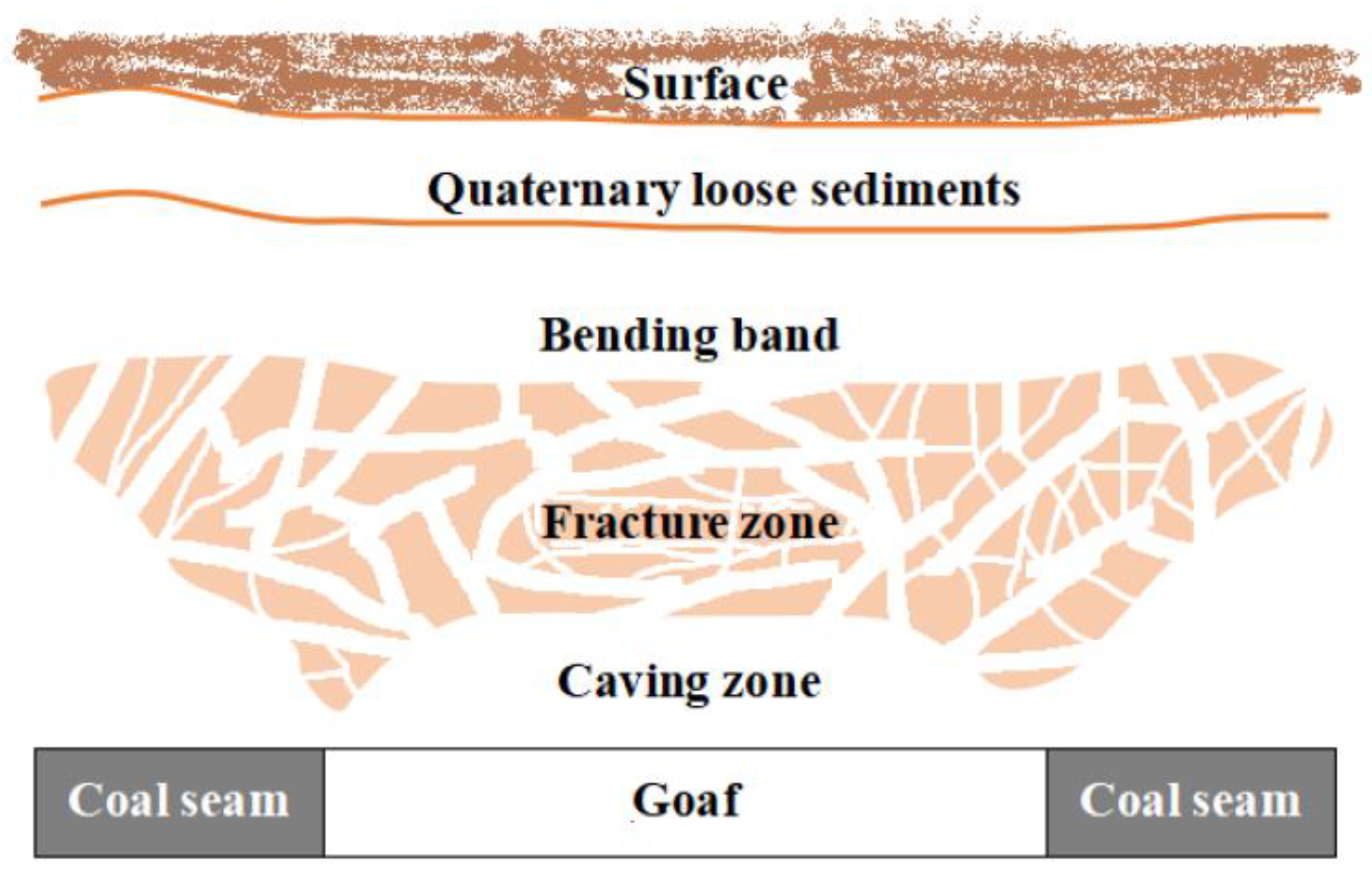
2.1. Typical Structure and Physical Properties of Coal Mine Goafs

Coal mine goafs often form after the mining process when the overlying strata collapse due to gravity. Generally, three zones are shaped vertically: the caving zone (overburden collapse of coal seam), the fracture zone (bending fracture under shear stress), and bending zone (from the roof of the fracture zone to the ground, deformed but not broken). See Figure 1 for details.

To facilitate the analysis of multiple types of coal mine goafs, for the purposes of this paper, two study areas were selected, as shown in Figure 2. These were located in the central part of Henan Province, China. Study Area 1 is bordered by Xinzheng City, Changge City and Yushi County, with a distance of 50 km from Zhengzhou City to the west of the city center. Study Area 2 is about 100 km away from Study Area 1. According to field investigation of the mining areas, the strata were deposited, from bottom to top, in the Paleozoic Cambrian and Middle Ordovician periods in the Upper Carboniferous Benxi Formation and, in the Taiyuan Formation, in the Permian and the Quaternary periods. The sedimentary sequence of coal seams is relatively clear and stable in the vertical direction and relatively uniform in the horizontal direction. The characteristics of resistivity parameters obtained from relevant sample tests are shown in

Table 2. Electrical parameters and lithological properties revealed by drilling data.

Lithology	Resistivity Distribution (Ω·m)	Distribution Stratigraphic Code	Remarks
Clay	50–200	Q	Quaternary
Sandstone	100–600	Q, P1s, C3t	Quaternary, Upper Carboniferous Taiyuan Group, Permian
Mudstone	30–100	Q, P1s, C2b	Upper Carboniferous Benxi Formation, Permian
Limestone	900–3900	O2f	Ordovician
Coal seams	1000–3000	P1s, C3t	Samples from the study area
Groundwater (mineralized water)	0.1–10

Note: The parameter values are measured from stable rock samples, and if the rock formations change, the actual stratigraphic parameters will change significantly.

. The resistivity value of coal seams is relatively high. After the resistivity value of coal seams, which was the highest found, the value of sandstone was second highest, and the value of clay rock was the lowest. Usually, the mineralization value of fractured water layers in the surrounding rocks of coal seams is up to 700–1100 mg/L, and aquifers often show abnormally low resistive distributions. In field surveys, coal mine goafs often form water-rich areas due to the groundwater infiltration or inflow through coal mine cracks. Taking typical structures and electrical characteristics into account, we designed theoretical models, as explained in the following sections.

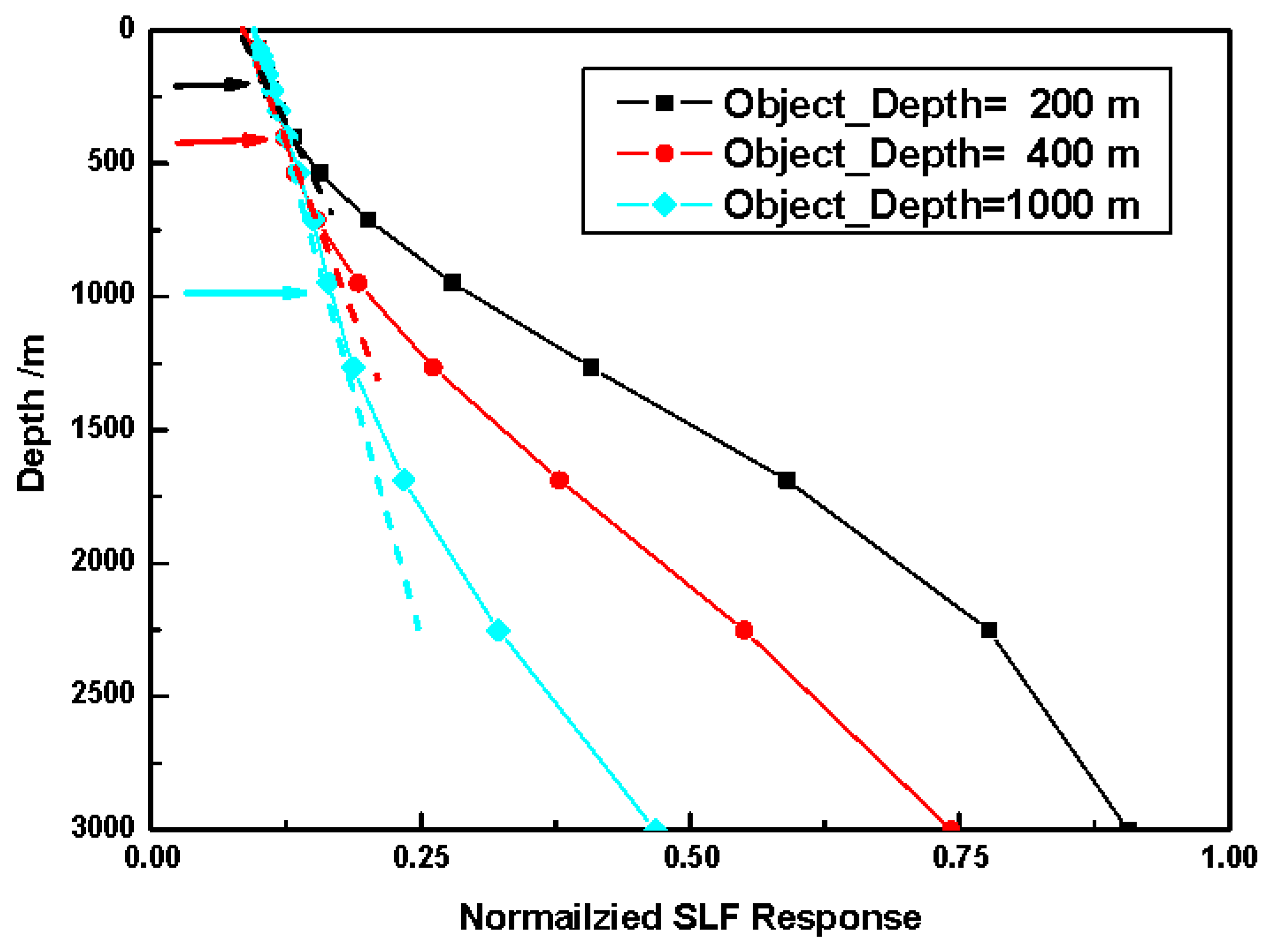
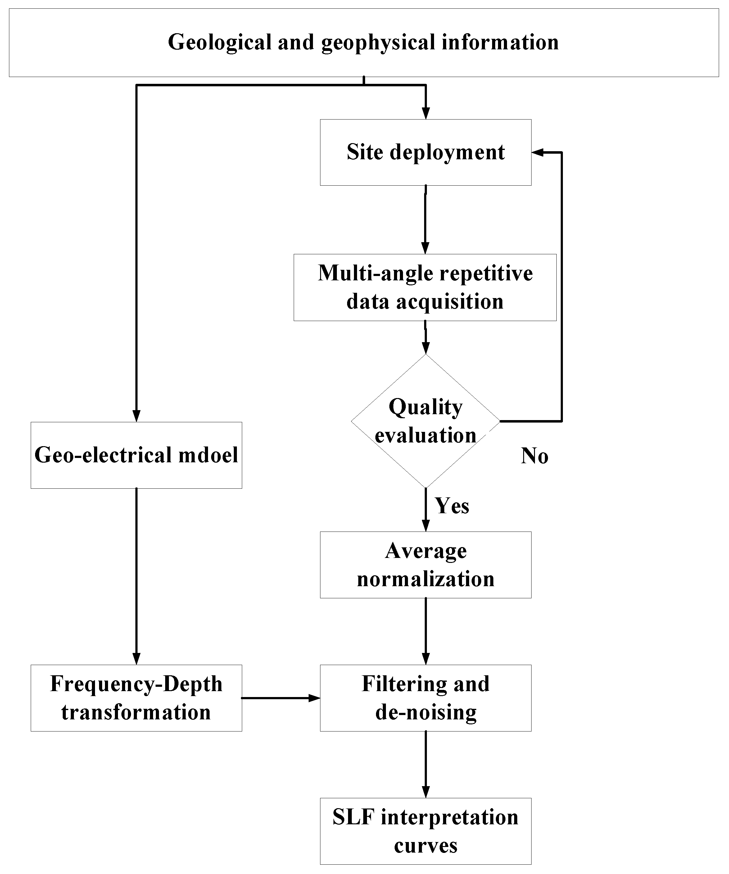
2.2. Semi-Quantitative Inversion of the SLF Method

As discussed above, electromagnetic inversion is the one of the key points of geo-electrical interpretation. For the SLF method, semi-quantitative inversion originates from the classical MT empirical formula, which accounts for how to realize frequency-depth transformation using magnetic component responses [32]. Firstly, Schmucker’s method describes the Schmucker impedance response by the first-order moment normalization of the induced current, and then completes the depth transformation according to the relationship between the impedance response itself and “apparent resistivity-phase”. However, this method is not valid for the case of a “low resistivity target layer + thick high resistivity basement”. Another classical empirical transformation, even more commonly used in the MT method, is Bostick inversion. As a semi-quantitative interpretation method, Bostick inversion is obtained following a mathematical transformation that analyzes the low-frequency asymptote of apparent resistivity under the conditions of both high-resistive limit and low-resistive limit. Equations (1)–(4) are modified from the references [32,40]. The general form derived from the intersection of two asymptotes is:

$$\rho \left(H\right)={\rho }_{\alpha }(\omega )\left[\frac{\pi }{2\phi \left(\omega \right)}-1\right]$$

(1)

$$H=\sqrt{\frac{{\rho }_{\alpha }\left(\omega \right)}{\omega \mu }}$$

(2)

In Equations (1) and (2), ρ(H) represents the inverted resistivity, and H represents the inversion depth. µ is the permeability, ω is the angular frequency. ρ_α(ω) and $\phi$(ω) are the apparent resistivity and phase at a certain angular frequency ω, respectively. Formula (2) is very similar to the exploration depth Formula (3) of the uniform half-space model [32]:

$$D=\sqrt{\frac{\rho }{\omega \mu }}$$

(3)

where D is the exploration depth, ρ is the uniform half-space resistivity.

In Equation (2), ρ_α(ω) is the apparent resistivity of two asymptotes at the intersection of a certain frequency. Usually, the apparent resistivity calculation depends on the impedance calculation, and the impedance of each frequency point is contributed by the underlying stratum excluding the target layer [42]. ρ_α is the comprehensive resistivity of each layer at the depth of asymptote intersections. The target layer and its underlying stratum can be treated as a uniform body with its compromise resistivity set as the comprehensive resistivity ρ_g. ρ_α can be replaced with the comprehensive resistivity ρ_g. The influence of depth range measurement can be measured using the weight coefficient, so the exponential parameter (corresponding distance weight coefficient) of ω in Formula (3) can be dynamically selected [40]. The improved frequency-depth transformation can customize the exploration depth range and reasonably extract the layer thickness. In the international system of units, the expression is:

$$H=356*\frac{\sqrt{{\rho }_g}}{f^c}$$

(4)

In Equation (4), H is the estimated depth (m), ρ_g is the comprehensive resistivity (Ω·m), f is the frequency (Hz), and c is the adjustable exponential parameter (index), i.e., the weight coefficient. This frequency-depth transformation is actually an interpolation method with the depth as the weight, which reflects the “volume effect” in the electromagnetic methods [40].

With regards to the fact that the depth of coal mine goafs is less than 1000 m, a three-layer model was designed with specific parameters described as the caprock layer (variable thickness, resistivity of 100 Ω·m), the middle target layer (100 m thick, variable resistivity) and the basement (infinite depth with resistivity of 1000 Ω·m). Different models were obtained by changing the buried depths and resistivity distributions of the intermediate target layer. For example, in the case of an intermediate target layer 100 m thick with resistivity of 1 Ω·m and a uniform half-space base of 1000 Ω·m, the comprehensive resistivity is set by test as 400 Ω·m, seen as a compromise between 1 Ω·m and 1000 Ω·m. The index parameter is manually set at 0.5 following multiple attempts according to the geological settings. The SLF amplitude responses at the midpoint of the surface of each model are calculated using one-dimensional forward modeling, as shown in Figure 3. When the buried depth of the target layer changes from 200 m to 1000 m, the theoretical responses can be directly transformed as the curves in the depth domain. Compared with the trend line (shown by the straight line), the starting position of the upturned tail basically corresponds to the top buried depth of the target layer. As shown by the arrows, when the buried depth of the middle layer is 200 m, the tail tends to tilt up from 200 m, which basically demonstrates that the semi-quantitative frequency-depth transformation is suitable for the buried depth estimation of the target layer. Meanwhile, the basement depth can also be reflected where the response tends to be gentle, around 2000 m. Therefore, the SLF response can be used for the delineation of the target layer in the estimated depth range.

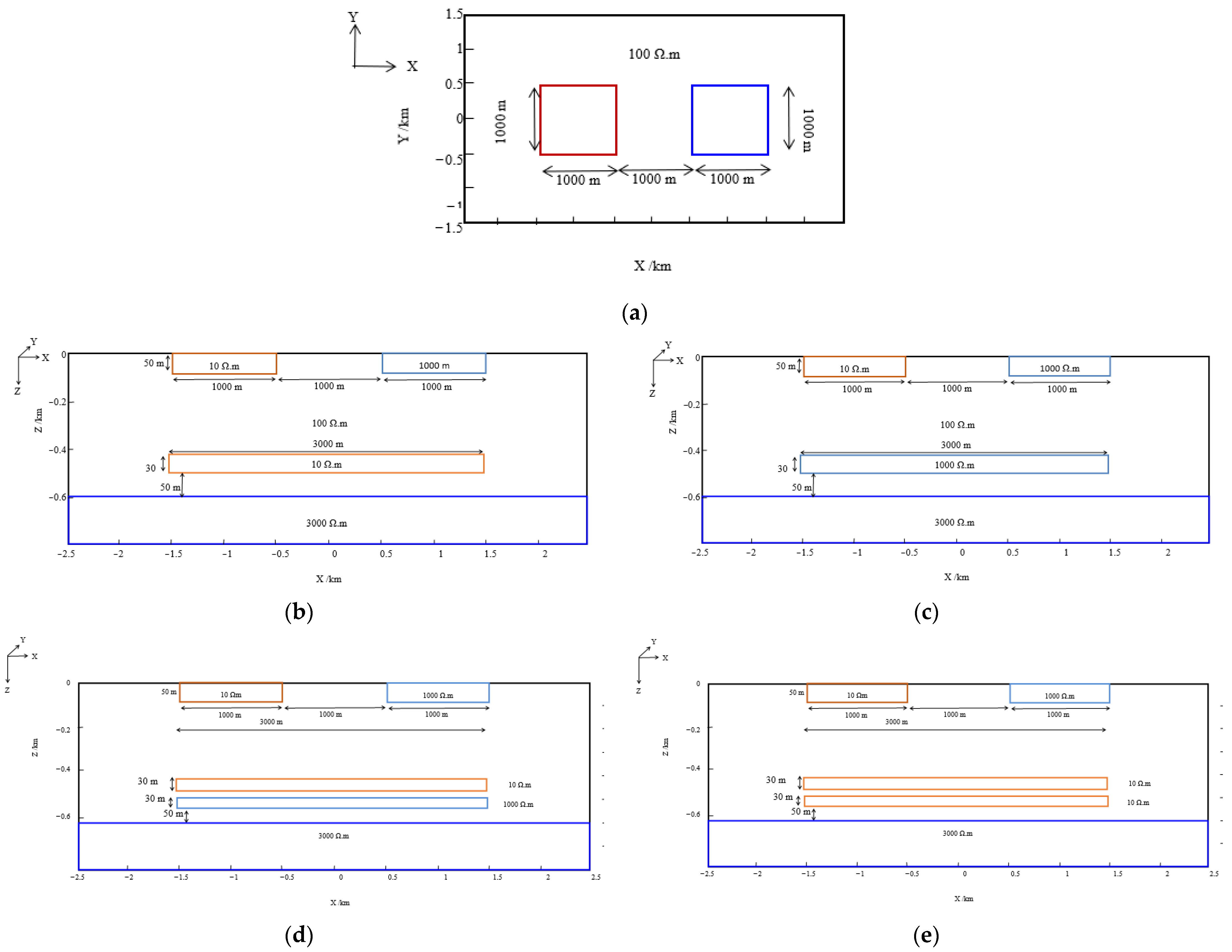
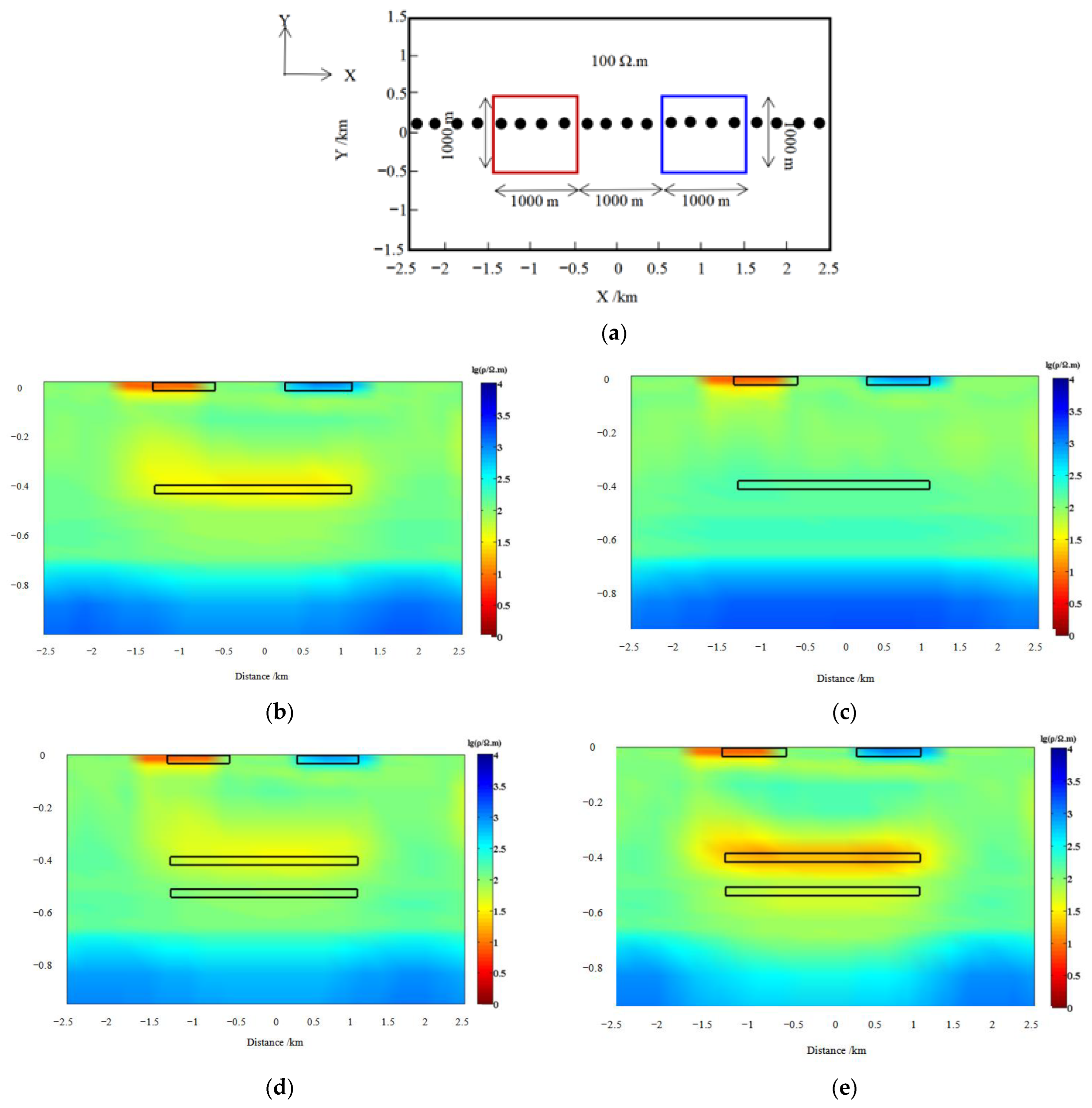
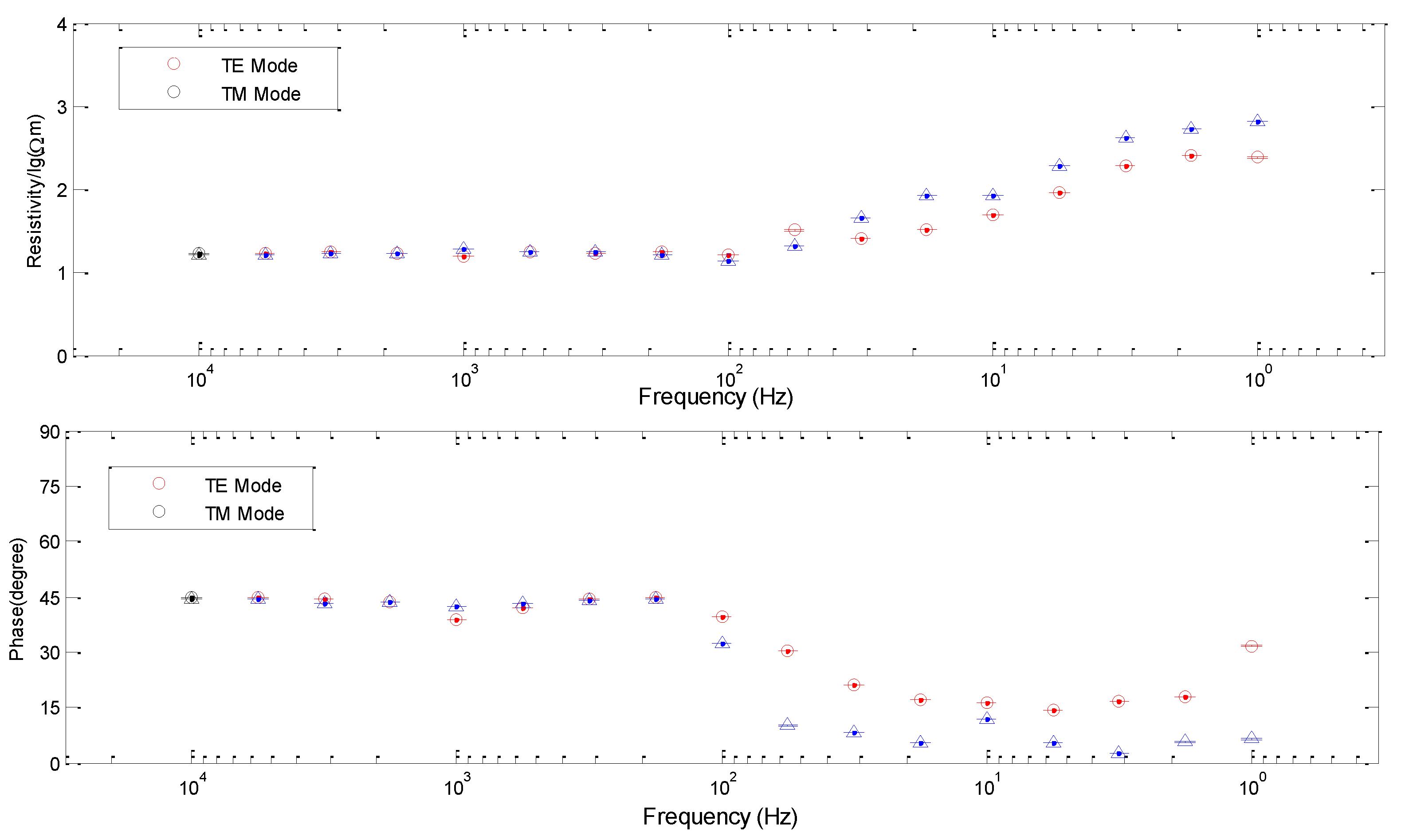
2.3. Three-Dimensional Electromagnetic Inversion of the AMT Method

AMT inversion is also theoretically explored for its feasibility in interpreting coal mine goafs. In the past years, the two-dimensional inversion of three-dimensional (3D) models has primarily been discussed. With the distributed three-dimensional inversion program entering the industrialization stage, it is no longer difficult to realize 3D inversion of real data in AMT exploration [41]. Considering that coal mine goafs usually belong to two extreme types—either complete high-resistive air-rich areas or complete low-resistive water-rich areas—models can be designed with two types of target layers embodied, which can be used to evaluate the feasibility of three-dimensional AMT inversion. Shallow surface electrical bodies regarded as typical 3D electrical anomalies are also considered, which are often far smaller than the AMT exploration scale of several kilometers to tens of kilometers. The target layer is often only tens of meters thick, which can be regarded as a thin layer relative to the buried depth (assuming that the “depth-thickness” ratio is not less than 10). The target layer is usually distributed along the strike and can be regarded as a two-dimensional structure. The electrical properties of basement and overlying sedimentary rocks are relatively stable and can be regarded as a one-dimensional structure. The buried depth of the target layers designed in this way is generally 400 m~700 m, and the thickness of the target layer is generally 10 m~50 m. In contrast, the shallow anomalies are also tens of meters thick. In order to distinguish the abnormal response from different stratum, the resistivity values of shallow anomalies and target layers were set as 10 Ω·m and 1000 Ω·m, respectively. The limestone basement was set as 3000 Ω·m. Synthetic models of thin low and high-resistivity target layers are shown in Figure 4. In Figure 4a, y is the strike direction of the stratum. At the surface of Z = 0 in the XOY profile, the area of interest was 5 km × 3 km, of which the surface anomalies were set as a scale of 1 km × 1 km with low resistivity (10 Ω·m) and high resistivity (1000 Ω·m). Along the XOZ section with y = 0, as shown in Figure 4b, the thickness of shallow abnormal bodies was 50 m. At a depth of 470 m, a two-dimensional anomalous body (3000 m × 30 m, 1 Ω·m) was designed as the exploration target layer extending infinitely along the strike Y direction. The high-resistive substrate at a depth of 50 m below the target layer was set as 3000 Ω·m. As for the high-resistivity target layer model, the design was almost consistent with that of the low-resistivity model, except that a two-dimensional high-resistive anomaly (3000 m × 30 m, 1000 Ω·m) was present in the XOZ section at y = 0, shown in Figure 4c. As for the mining area, there are often multiple target layers (coal seams or goafs), and, therefore, two-layered target models were also designed with a particular depth distance. The first layer was set as a low-resistive layer and the second layer was set as a high-resistive or low-resistive layer; these models were also used to test the AMT 3D inversion, as shown in Figure 4d,e.

A typical measurement line, which strides over a shallow inhomogeneous body at Y = 0 in the XOY plane, as shown in Figure 5a, was selected. The impedance tensor responses of 20 points along the line were simulated by 3D forward modeling. For each response, 5% Gaussian random noise was added. The synthetic data were treated as the initial data file of the 3D inversion. Then, the 3D impedance tensor inversion of the line was performed using the ModEM inversion system [48]. Both the initial model and the priori model were set to a uniform half-space of 100 Ω·m. The 3D inversion grid was set to 24 × 32 × 28, and the air layer was divided into 7 grids. The horizontal grid profiles were carried out in 250 m steps in the region of interest. In the vertical Z-direction, the shallow surface and target layers were dissected in 10 m grid steps. Meanwhile, the surrounding layers were dissected at 25 m–100 m intervals, and so that the substrate depth meets the minimum frequency skinning depth and boundary conditions. The initial RMS of the 3D inversion was 10, on average, and the final RMS was about 1.5–2 after 80–100 iterations when the final iteration converged. The results of 3D tensor impedance inversion for all points of the same line are shown in Figure 5b–e, where all the superficial anomalies can be accurately circled. In Figure 5b, the low-resistive target body is clearly prominent. However, there are still some false anomalies in the vertical direction of the target layer, which may be related to the excessive thickness and the low-resistive influence of the surface anomalies. The model inversion procedure in the “high-resistive target layer” model is the same as that of the low resistive model in the previous section; the inversion results are shown in Figure 5c. Both the resistivity distribution and anomalous boundary can be accurately extracted for the shallow anomalies. However, it is very difficult to distinguish the high-resistive target layer from the background. This demonstrates that it is difficult to extract the high-resistive thin layer in the 3D impedance tensor inversion of the AMT method, and it is not suitable to use the high-resistive thin layer as the target. Therefore, taking into account the available computational resources, it is better to choose the 3D inversion of a thin low-resistive target layer in the AMT exploration, which can achieve the purpose of highlighting the targets as much as possible and reducing the influence of false anomalies.

The 3D inversion results of the “two target” models are further discussed in Figure 5d. When the first layer is low resistive, the high-resistive anomalies below will be completely masked. If the lower layer is a low-resistive anomaly, the inversion effect of the first layer will be enhanced, and it will be difficult to infer the lower anomaly, as shown in Figure 5e. All of the results show that it is almost always easier to completely invert the shallow anomalies. Although both the boundary and resistivity values of the target layer can be inverted, there is still a small vertical resistivity bias in the inversion. In the exploration depth range of the AMT method, the vertical distribution of the area of interest in models is 1000 m deep. As for the target layer at tens or hundreds of meters, the inversion results will be affected by the inversion algorithm, calculation accuracy and shallow surface anomalies. Even under ideal circumstances, it is very likely that electrical deviations of several meters or even a dozen meters from the target layer will be caused, which cannot be completely avoided in practical applications. Therefore, the AMT method is suitable for 3D inversion interpretation of single-layer conductive anomalies. In addition, we conducted a stability test of 3D inversion with different initial models and error bars, including full-information (impedance tensors + tippers) inversion. The results demonstrate that full-information 3D inversion does not provide more target information than that of impedance tensor inversion. Additionally, the initial model plays a key role in 3D inversion. However, there is not sufficient empirical evidence to demonstrate that the initial model would be better on the AMT sounding scale. In practice, the uniform half-space model is usually chosen as the initial model, or one-dimensional inversion is performed and interpolated based on real data [48].

Coal mine goafs often form water-rich areas due to groundwater infiltration or inflow, and low-resistive anomalies can be considered as targets. Through the theoretical analysis above, the aforementioned electromagnetic methods were also appropriately applied in our coal mine goaf areas. In the mining or coal retrieval areas, there is an urgent need to improve the geological discrimination of geological threats and water-rich damages, such as coal seams, fault positions and caves. In the following section, the actual application will be discussed in detail.

3. Collapse-Type Coal Mine Goaf Interpretation

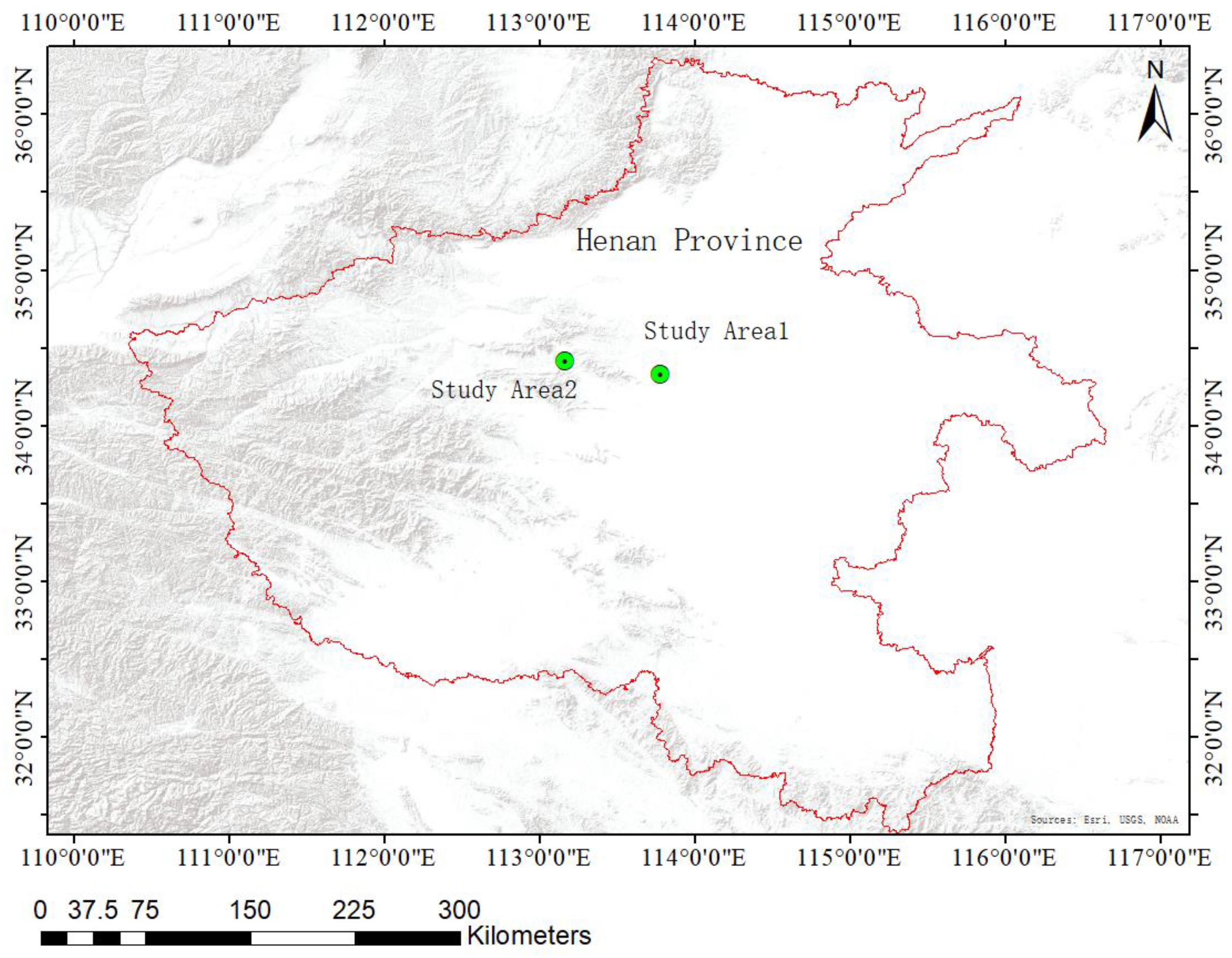
3.1. Overview of the Collapse-Type Mining Area

This area is located in Study Area 1 (shown in Figure 2), where the whole tectonic pattern is an incomplete asymmetric diagonal structure with an axial direction from NE to SW. For collapse-type mining area, two folds were distributed and about 82 faults with a drop greater than 5 m were identified, all of which were high-angle positive faults with a fault density of 1.48 faults/km². A field survey should be carried out to reveal the status of faults which lie concealed around coal mine goafs, as shown in

Table 3. Statistical characteristics of faults in collapse-type coal mine goaf area.

Fault ID	Fault Feature	Extension Length (m)	Bed Attitude			Stratigraphic Fall (m)	Corresponding Sites
			Strike	Dip	Dip Angle
F13	Positive	1700	Near EW	S	65°	0~15	8–10
F12	Positive	>3600	NWW~SEE	NNE	65°	0~60	8–10
F11	Positive	4300	NWW~SEE	NNE	65°	0~175	13–15
F10	Positive	1050	NWW~SEE	SSW	65°	0~70	16–17

. Additionally, the stratigraphic formations, from old to new, revealed by boreholes, belong to the Ordovician’s Majiagou Group, the Upper Carboniferous’ Taiyuan Group, the Lower Permian’s Shanxi Group and Lower Shi Box Group, the Upper Permian’s Upper Shi Box Group and the Quaternary Formation. The Carboniferous and Permian formations are the main coal-bearing seams.

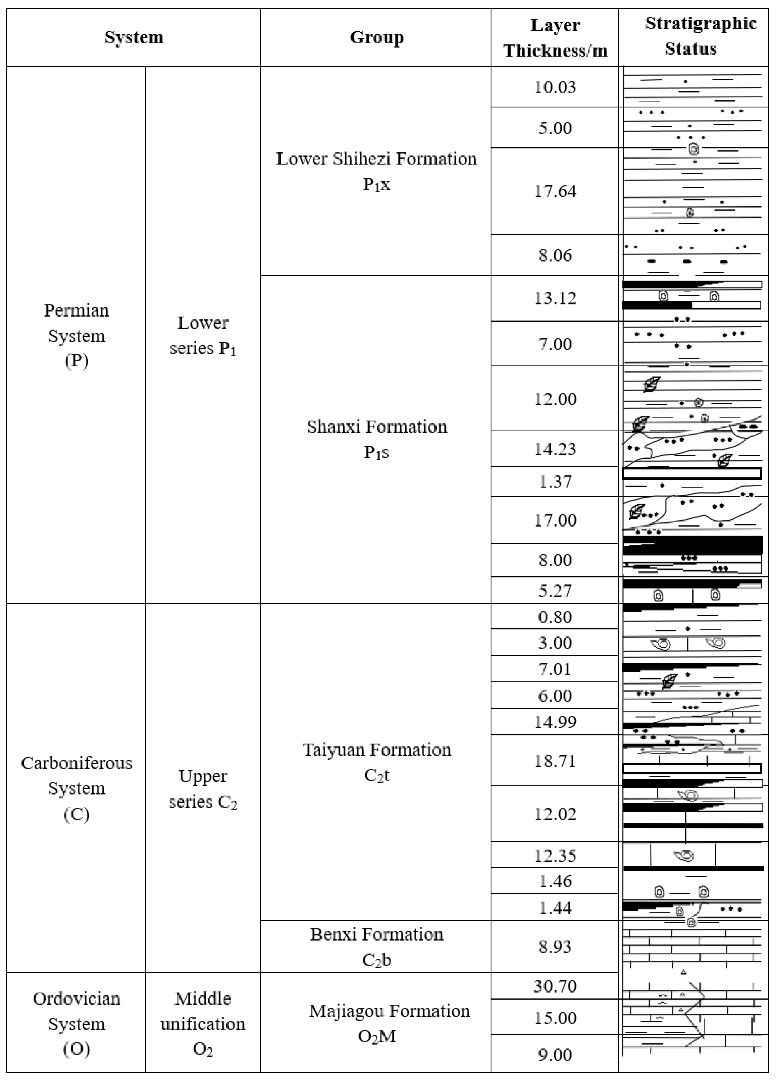
3.2. Stratigraphic Characteristics and Preliminary Exploration Basis

The coal-bearing strata in this area were mainly distributed in the Taiyuan Group, Shanxi Group, Lower Shi Box Group and Upper Shi Box Group, and the total thickness of coal seams was 8.14 m. The No. 2_1 coal seam is the main minable coal seam. At this location, it is scarcely possible to distinguish the mining area from the surrounding rocks. However, the overlying aquifer of the No. 2_1 coal seam forms the direct water filling source, and this may have a hydraulic connection with other strong aquifers and coal mine goafs. The fracture water enters the working faces as the mining process occurs; this can form a low-resistive zone. This zone was quite closely related to the faults, and the fracture water status and fault distributions in the collapsed mining area must be accurately measured before the successive mining plan is initiated.

3.3. The SLF Exploration Tests

High-quality detection data are important to improve SLF signal resolution and inversion accuracy. In recent years, a high-precision and portable device used in the SLF method has been developed; a workflow for the field survey is summarized in detail. For the acquisition of data in the SLF band, a BD-6 electromagnetic detector developed by us is mainly used [40]. The detector uses a high-precision magnetic sensor to receive a horizontal magnetic field component signal from 3 Hz to 3000 Hz. The system consists of three parts: a magnetic sensor, a host and a power supply. The magnetic sensor contains a magnetic rod, an amplification circuit, a programmable trap circuit, a high-speed acquisition circuit and other modules. The minimum received induced voltage value is 0.1 μV, and the response of the weak varying magnetic field amplitude can be obtained sensitively. The sensor noise is very faint, and the preamplifier output gain can amplify the weak signal at micro-voltage level by 10⁶ times, which provides hardware support for the effective signal identification. The host contains data acquisition, format conversion, storage and control units, and is capable of suppressing powerline noise (50 Hz) and its harmonics. The power supply unit can supply power to the host and the sensor for a long time. The equipment is portable, easy to use and highly efficient.

The workflow of the SLF method is shown in Figure 6. In a specific study area, suitable measurement points are selected according to real data, and the BD-6 detector is used for multiple, multi-angle data acquisitions. The data quality is evaluated after each acquisition; a high signal-to-noise ratio and good spectral repeatability are required. Through the averaging, normalization, filtering and denoising to suppress the powerline interference, the effective geological information is highlighted with semi-quantitative inversion. In fact, it is necessary to, firstly, evaluate the resistivity distributions of the target layer and the following strata from known geological and geophysical data. The empirical parameter of the improved frequency-depth transformation in Section 2.2 is often not more than 0.5 when the target layer is of low resistivity. In the study area, the electromagnetic detection test was carried out for production monitoring from 27–28 April 2012. The detection depth, step size, magnification, probe orientation and wiring plan were initially determined according to the actual conditions. A total of 26 measurement sites were selected from north to south at intervals of about 20 m—as far as possible from the surrounding human noise.

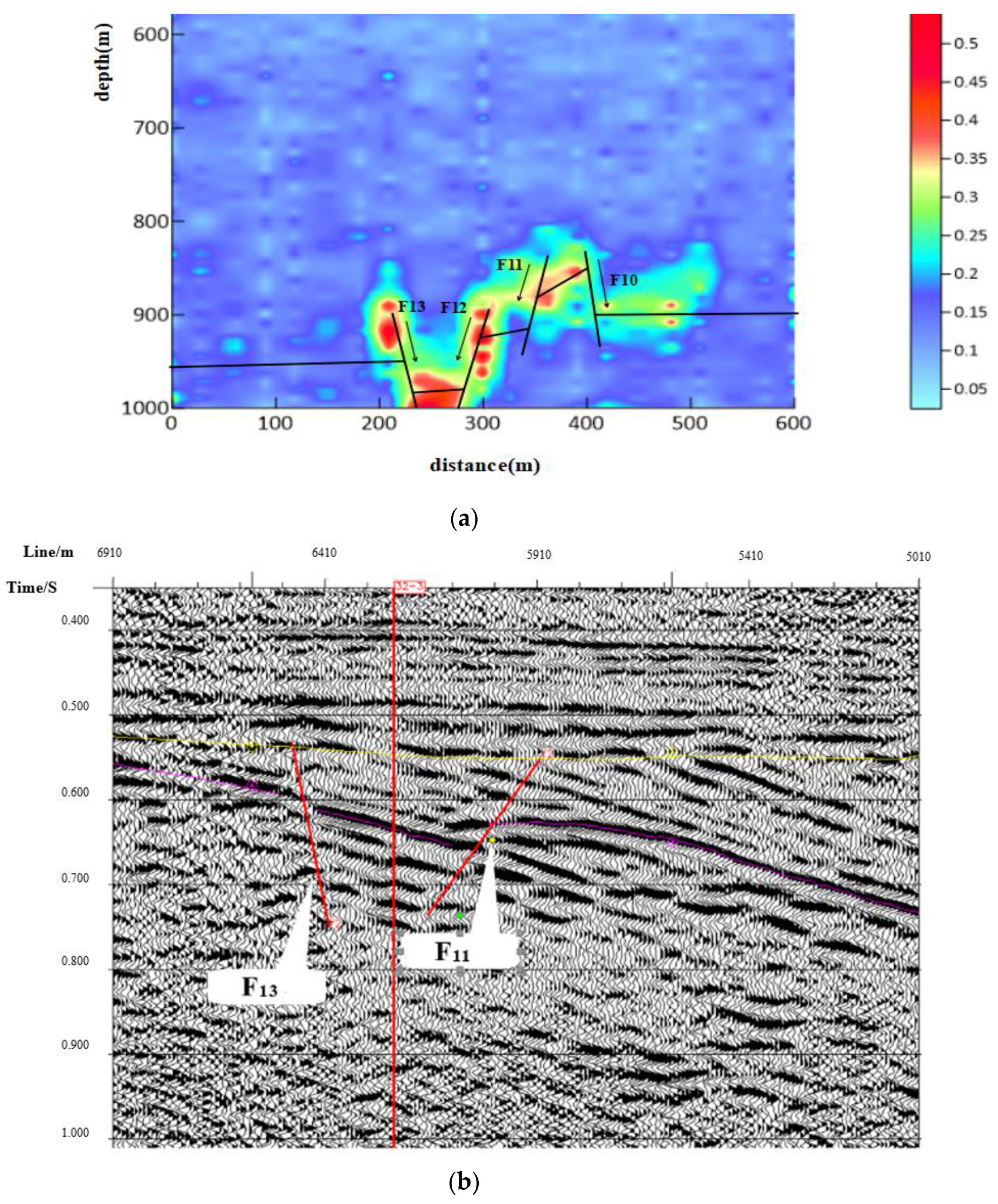
3.4. Result Interpretation and Comparative Validation

The semi-quantitative inversion profile of the SLF method was obtained from the left to the right of No. 8–16 sites, as shown in Figure 7a. The anomalous response in the curve was mainly around 900 m, which may be due to the conductive difference between the upper and lower layers. The response section demonstrated that there were indeed faults at measurement sites 08–10 and sites 13–16. The low-resistive layers in the different depths of 500–700 m formed because of faults, which led to the anomalous responses at dislocated depths. The drilling data show that the coal seam is located at a depth of 590–610 m, which is mostly consistent with the exploration results. Combined with the 2D seismic travel time profile (Figure 7b), the faults were also interpreted based on the distortion or misalignment of the reflection waves, corresponding to significant interruptions or disappearances of the coal seams. The profile showed that the stratum above the yellow line was horizontally distributed, and, meanwhile, the reflection waves below demonstrated a misalignment of the seismic events, where there are interruptions and disappearances at the faults. The reflection waves on the left and right sides were clearly different, which indicated that there were some electrical differences between two sides of the faults. The characteristics of the faults in the profile were similar to those of the SLF interpretation. The misalignment of F13 and F11 faults was consistent with the fault characteristics. In contrast, F12 and F10 were also further revealed in this SLF profile. Thus, the SLF method can feasibly reflect the hidden fault distribution with more details than that of the 2D seismic method.

According to the geological data of the study area, F12 is located north of F11, in the northwestern part of the study area. F11 starts from Xiaolianlou village in the west and passes through Xiaofanzhuang village in the north. F10 is located in the central part of the study area, starting from Lions Xing village in the west and ending at the F11 fault in the east, which is basically consistent with the SLF-interpreted distribution. The F13 fault is a positive fault with an extension of 1700 m, trending nearly east–west and tilting southward with a dip angle of 65°. It intersects with the positive F12 fault, which extends more than 3600 m, trending north–west–west with a maximum drop of 60 m. This shows that these two faults have been verified by the mine production units, and the distribution of faults at this location is indeed consistent with the predicted depth range. This shows that the SLF electromagnetic method is effective for the rapid estimation of collapse-type mining areas.

4. Water-Rich Type Coal Mine Goaf Interpretation

4.1. Overview of Hydraulic-Threat Coal Mining Areas

There are a few water-type coal mine goafs located in Study Area 2 (shown in Figure 2), where two mining areas were selected for AMT exploration tests. The stratigraphy of the No. 01 mining area is dominated by a sedimentary rock system, and the main geological structure is a broad and gentle anticline with a dip angle 3–15° and an axial NWW–SEE direction. This anticline controls coal seam production in the northern part of the mining area with some wide and gentle folds. Tens of kilometers away from area No. 01, the No. 02 mining area is sandwiched between two major anticlines: Songshan and Minshan anticlines. The structure is generally characterized by a broad and gently incomplete syncline. The northwest of coal mining area No.2 is generally high, but lower in the southeast, with a highest elevation of 470 m. The two coal mining areas face upwards with a high water-damage risk, which has resulted in great challenges for the coal mining process.

4.2. Stratigraphic Characteristics and Coal-Water Distribution

The stratigraphic development of the two coal mining areas is deposited, from bottom to top, from the Paleozoic Cambrian in the Ordovician Middle Majiagou Group, from the Carboniferous in the Upper Benxi Group, and, in the Taiyuan Group, from the Permian and the Quaternary, as shown in Figure 8. The main coal seams in the Permian Shanxi Group are mainly mined at a depth of 200–400 m, with an average seam thickness of 4.86 m. According to the field survey, the fissure water source in the mining area was mainly from the roof aquifer, and water bursts have occurred many times. The main water-bearing layers, with regards to the minable No. 2_1 coal seam, were as follows. Firstly, the Upper Carboniferous Taiyuan Group aquifer, consisting of 4 layers of limestone, from L1 to L4, with a thickness of 13.86~42.99 m. The average distance of this aquifer section from the bottom of the No. 2_1 coal seam was 40~60 m; this aquifer is an indirect water-filled aquifer. The roof-fractured aquifer of the No. 2_1 coal seam was initially stable because of the significant thickness of the overlying aquifer and large static storage capacity. However, the original status of the sliding tectonic zone was destroyed along with the mining of this coal seam, which directly led to a connection between the overlying caving zone and sandstone aquifers. In the later stage of mining, aquifuges can be greatly weakened by damage to the working face. This may pose a hydraulic threat to the mining of the working face, leading to the demand for detection of these weaknesses by the AMT method, as described in the following sections.

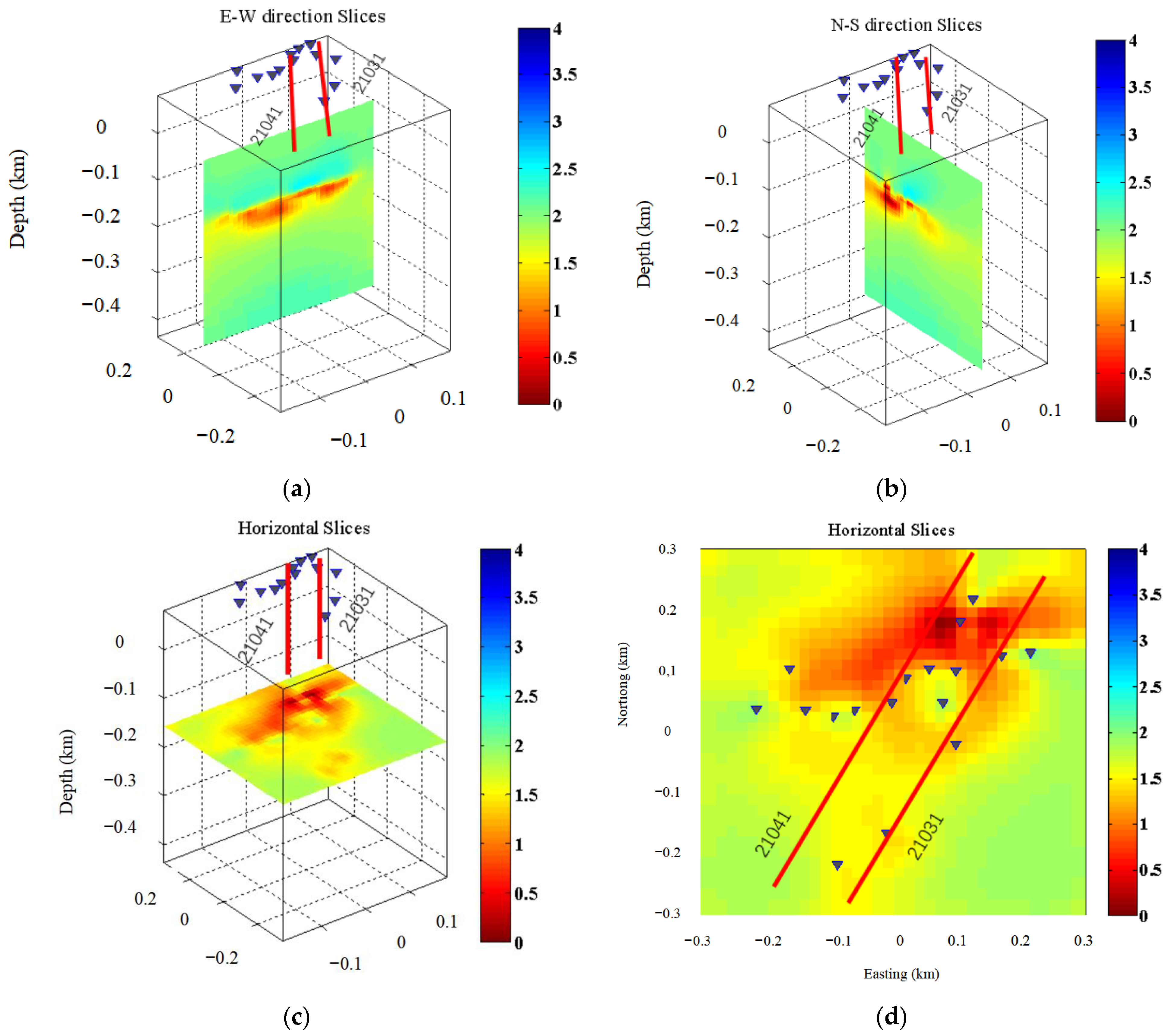
4.3. AMT Data Acquisition and 3D Inversion

The AMT module of the V8 multifunctional electromagnetic device from Phoenix Geophysics Ltd., Toronto, Canada has been used to fulfill the field survey of water-rich coal mine goafs. The data from the working face of the No. 1 mining area was collected in August 2013, and the survey was carried out to allow the measuring line to cover the main mining face. The observation time for each measurement site was one or two hours. In late June 2014, data collection was also carried out along the working area of the No. 2 mining area. The measurement sites were geographically distributed in a straight line. The surrounding area was mostly covered by farmland, with no interferences from the AMT module. The distance between the sites was basically from 30 m to 50 m. In Figure 9, the AMT’s apparent resistivity and phase curves of a field survey site showed that a nearly consistent trend was similar to the responses of the one-dimensional stratified model. However, at the low frequency stage (below 10 Hz), it showed two-dimensional characteristics. In a word, the stratigraphic distribution in these areas is simple and homogeneous, but they need to be accurately interpreted by subsequent 3D inversion.

4.4. Results and Discussions of the No. 01 Mining Area

The coal seam in the No. 01 mining area is relatively stable; No. 21041 is the first comprehensive mining face. The coal seam’s elevation is −190 to −120 m with a surface elevation from +225.3 to +296 m. The average coal thickness is 4.7 to 5.3 m. The water-bearing layer, 25 to 85 m thick, is 20 to 100 m high from the coal seam roof. The water richness of the aquifer is unevenly distributed in No. 21041, and the similar working face No. 21031 is located to the west. The measurement sites almost cover the two working faces as far as possible, as shown in Figure 10. In Figure 10a,b, the 3D inversion slices extracted from the E-W and N-S directions can be further cross-checked with each other. The inversion results also show that there is a clear low-resistive distribution in the depth range of 280 m to 400 m. Especially in the NE part of the working faces, the conductive area is characterized by larger thickness and lower resistivity, which is probably due to the presence of a hydraulic fracture zone. According to the drilling data, there is a heavily water-filled upper roof aquifer adjacent to No. 21041. Therefore, the roof fracture permeability is likely related to the surrounding hydraulic conductivity structures and has probably already posed a threat to coal mining in the past.

In order to illustrate the detection results more clearly, we intercepted the resistivity cross-section slice of 310–320 m, as shown in Figure 10c,d. The No. 21041 comprehensive mining face is located in the middle of the profile, and the roof of the coal seam is water-rich with fissure water. The field survey demonstrates that the roof water has entered the coal mine goafs along the fissure zone during the mining process. This could also be verified by an in situ sampling test, revealing that the bottom slab of the coal seam was not affected and has been reinforced by grouting operations in recent years. Therefore, the water is deduced to originate from the roof fissures. The upper part of the cross-section, as shown in Figure 10d, shows a very clear low-resistive distribution. This likely indicates that the overlying fissure permeability zone of the goafs has been located; this is also consistent with the distribution of the No. 21041 and No. 21031 mine passages. Furthermore, this may cause a permeability hazard to subsequent mining. In the lower part of the profile, there is no hydraulically permeable area, which is also consistent with the actual mining situation. Additionally, the drilling data revealed that the main No. 2-1 coal seam distribution depth was 340 m–400 m, and the roof aquifer was located 20–100 m above it. This is also consistent with the low-resistive anomaly distribution from 250 m to 400 m indicated by 3D inversion, and the local distribution of suspected water-rich goafs also corresponds to the inferred depth range of the coal seam.

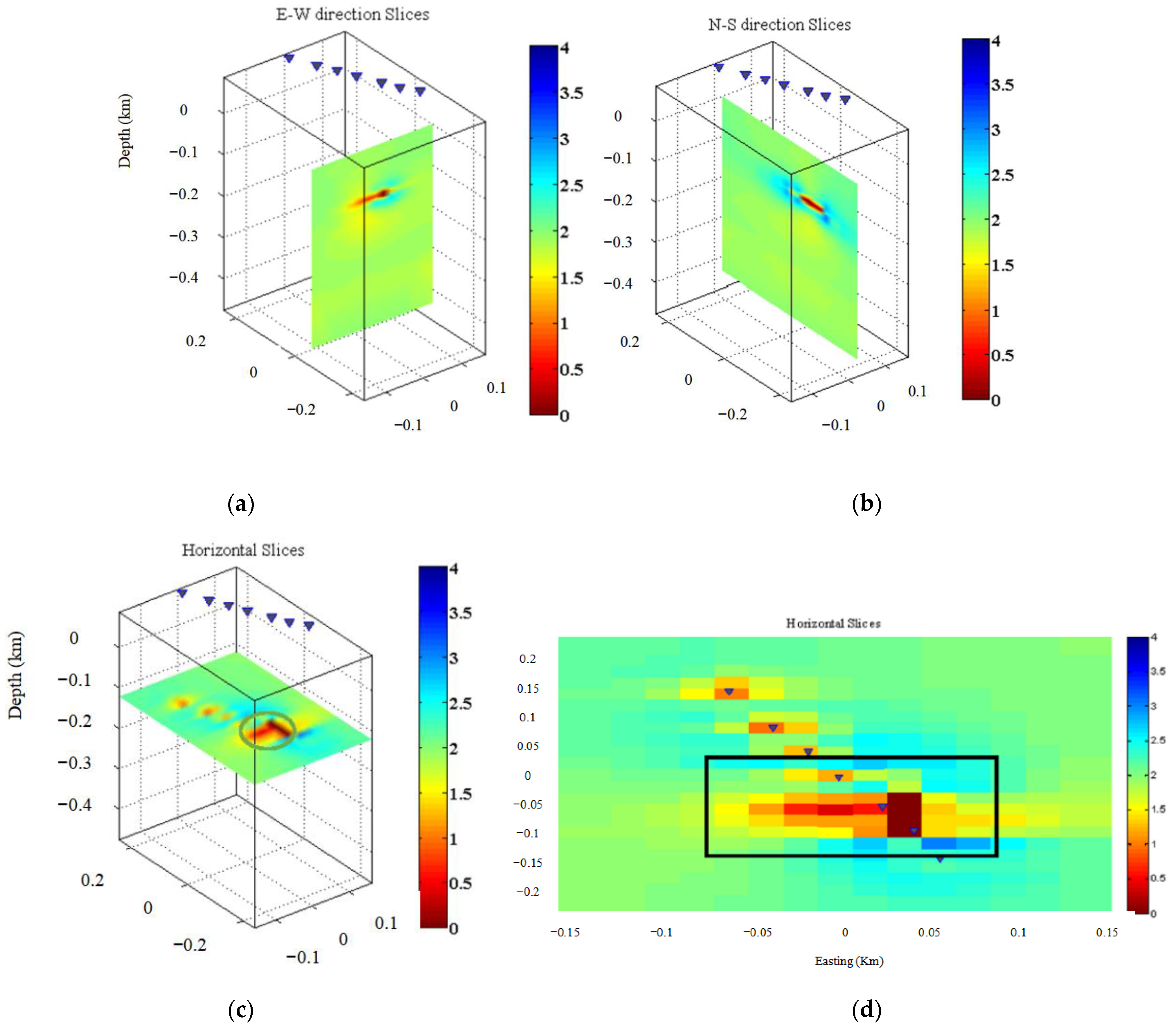
4.5. Result Analysis of the No. 02 Mining Area

The working face No. 12201 in the No. 02 mining area was selected as the main water-rich type goaf target. This working face involves Neoproterozoic strata, and the fallout fracture zone could reach the Neoproterozoic bottom “sand-gravel” aquifer. The distribution of the total thickness of the Neoproterozoic sandstone layer has been damaged by mining; fractures were found in the bottom 0–50 m of the rock. The working face spread towards the east through the fold axis, and the hydraulic permeability zone formed because of the gradually intensive fracture of the aquifers at the bottom of the Neoproterozoic system. This may cause water from the bottom of the Neoproterozoic system to enter the mining area, thus threatening the safety of mining operations.

The finite difference method was used for 3D forward modeling, and the resistivity sections of each depth layer were obtained by 3D inversion; the anomalies were sliced along the east–west, north–south and horizontal directions of the sectioning grid, as shown in Figure 11a–c. It can be seen that there is a clear distribution of low-resistive anomalies at the depths between 100 m and 200 m. Especially around sites circled in Figure 11c, the distribution of low-resistive anomalies was particularly obvious, with lower resistivity values and a wider distribution. As shown in Figure 11d, there was an obvious conductive area between measurement sites (circled in the black box). Considering that the working face is located in the axis of the Hutuo anticline, the coal seam is covered by the slightly water-rich Neoproterozoic aquifer. It can be inferred that the water source of the low-resistive area may come from the overlying zone. According to a comprehensive analysis, the No. 12211 working face caused the fractured zone to fall to the bottom of the Neoproterozoic aquifer at nearly 150 m depth, which resulted in the aquifer’s connection with the coal seam. Finally, a hydraulic connection between the Neoproterozoic aquifer and the coal seam formed. In order to reduce the damage from roof fracture and the damage of the lower Neoproterozoic aquifer, it is recommended to strengthen the monitoring of the roof water level and the water influx after mining, especially to prevent the formation of a suspected water-filled area (shown by the rectangle box) at depths between 100 m and 150 m. These exploration tests successfully guided the subsequent mining plan.

5. Conclusions

This paper proposes and illustrates a goaf interpretation trend using passive electromagnetic methods (especially for the SLF method and the AMT method). The effectiveness of these methods has previously been validated in theory and practice, which lays a foundation for the future popularization of the electrical delineations of goafs. Some key concluding remarks:

(1)

Geo-electrical goaf models were designed and the theoretical feasibility of interpreting goaf targets was fully explored by developing forward modeling and inversion algorithms using the finite difference method (FDM).

(2)

Semi-quantitative inversion of the SLF method was fully explored with a three-layer electrical model, which can efficiently perform the vertical delineation of low-resistive bodies and facilitate fault structure identification.

(3)

Theoretical 3D inversion analysis of “single and double target” models has been discussed systematically, and this AMT method, with appropriate initial models and data accuracy selections, was most appropriate for single low-resistive layer distribution at a depth range of 100 m–400 m.

(4)

In field surveys of goaf areas, the inverted depth distributions using both methods are basically consistent with the water-filled goafs and surrounding layers, as verified by known data. SLF interpretation was successfully applied in collapse-type mining goaf areas. In contrast, with regards to water-rich-type coal mine goafs, the AMT method, using stable 3D inversion, has the capability of revealing obvious low-resistive anomalies appropriate for determining the hydraulic tectonic area connected with fracture zones. These results can help industries to improve subsequent coal production.

In the future, a joint use of these passive electromagnetic methods should be investigated more thoroughly; a set of economic and rapid goaf evaluation methods should be the subject of greater practical attention for subsequent mining areas under study.

References

1. Gui, H.; Qiu, H.; Qiu, W.; Tong, S.; Zhang, H. Overview of Goaf Water Hazards Control in China Coalmines. Arab. J. Geosci. 2018, 11, 1–10. [Google Scholar] [CrossRef]
2. Guoqiang, X.; Hai, L.; Weiying, C. Progress of Transient Electromagnetic Detection Technology for Waterbearing Bodies in Coal Mines. J. China Coal Soc. 2021, 46, 77–85. [Google Scholar]
3. Yin, Y.; Zhao, T.; Zhang, Y.; Tan, Y.; Qiu, Y.; Taheri, A.; Jing, Y. An Innovative Method for Placement of Gangue Backfilling Material in Steep Underground Coal Mines. Minerals 2019, 9, 107. [Google Scholar] [CrossRef] [Green Version]
4. Chlebowski, D.; Burtan, Z. Geophysical and Analytical Determination of Overstressed Zones in Exploited Coal Seam: A Case Study. Acta Geophys. 2021, 69, 701–710. [Google Scholar] [CrossRef]
5. Wang, Y.; Fan, X.; Niu, K.; Shi, G. Estimation of Hydrogen Release and Conversion in Coal-Bed Methane from Roof Extraction in Mine Goaf. Int. J. Hydrogen Energy 2019, 44, 15997–16003. [Google Scholar] [CrossRef]
6. Xinhai, Z.; Hui, Z. Prediction Method of Coal Mine Goaf Temperature and Its Practical Application. IOP Conf. Ser. Earth Environ. Sci. 2021, 647, 12008. [Google Scholar] [CrossRef]
7. Xie, H.; Gao, M.; Zhang, R.; Peng, G.; Wang, W.; Li, A. Study on the Mechanical Properties and Mechanical Response of Coal Mining at 1000 m or Deeper. Rock Mech. Rock Eng. 2019, 52, 1475–1490. [Google Scholar] [CrossRef]
8. Yu, C.; Wang, Z.; Tang, M. Application of Microtremor Survey Technology in a Coal Mine Goaf. Appl. Sci. 2023, 13, 466. [Google Scholar] [CrossRef]
9. Xue, G.Q.; Pan, D.M.; Yu, J.C. Review the Applications of Geophysical Methods for Mapping Coal-Mine Voids. Prog. Geophys. 2018, 33, 2187–2192. [Google Scholar] [CrossRef]
10. Zhang, S.; Sun, L.; Qin, B.; Wang, H.; Qi, G. Characteristics and Main Factors of Foam Flow in Broken Rock Mass in Coal Mine Goaf. Environ. Sci. Pollut. Res. 2022, 29, 47095–47108. [Google Scholar] [CrossRef]
11. Zhang, C.; Tu, S.; Zhao, Y.X. Compaction Characteristics of the Caving Zone in a Longwall Goaf: A Review. Environ. Earth Sci. 2019, 78, 1–20. [Google Scholar] [CrossRef]
12. Zhang, X.X.; Ma, J.F.; Li, L. Monitoring of Coal-Mine Goaf Based on 4D Seismic Technology. Appl. Geophys. 2020, 17, 54–66. [Google Scholar] [CrossRef]
13. Zhu, G.A.; Dou, L.M.; Cai, W.; Li, Z.L.; Zhang, M.; Kong, Y.; Shen, W. Case Study of Passive Seismic Velocity Tomography in Rock Burst Hazard Assessment During Underground Coal Entry Excavation. Rock Mech. Rock Eng. 2016, 49, 4945–4955. [Google Scholar] [CrossRef]
14. Zhou, B.; Deng, C.; Hao, J.; An, B.; Wu, R. Experimental Study on the Mechanism of Radon Exhalation during Coal Spontaneous Combustion in Goaf. Tunn. Undergr. Sp. Technol. 2021, 113, 103776. [Google Scholar] [CrossRef]
15. Xiang, Z.; Si, G.; Wang, Y.; Belle, B.; Webb, D. Goaf Gas Drainage and Its Impact on Coal Oxidation Behaviour: A Conceptual Model. Int. J. Coal Geol. 2021, 248, 103878. [Google Scholar] [CrossRef]
16. Li, L.; Qin, B.; Liu, J.; Leong, Y.-K.; Li, W.; Zeng, J.; Ma, D.; Zhuo, H. Influence of Airflow Movement on Methane Migration in Coal Mine Goafs with Spontaneous Coal Combustion. Process Saf. Environ. Prot. 2021, 156, 405–416. [Google Scholar] [CrossRef]
17. Yang, C.; Liu, S.; Wu, R. Quantitative Prediction of Water Volumes Within a Coal Mine Underlying Limestone Strata Using Geophysical Methods. Mine Water Environ. 2017, 36, 51–58. [Google Scholar] [CrossRef]
18. Wu, G.; Yang, G.; Tan, H. Mapping Coalmine Goaf Using Transient Electromagnetic Method and High Density Resistivity Method in Ordos City, China. Geod. Geodyn. 2016, 7, 340–347. [Google Scholar] [CrossRef] [Green Version]
19. Xu, X.; Peng, S.; Yang, F. Development of a Ground Penetrating Radar System for Large-Depth Disaster Detection in Coal Mine. J. Appl. Geophys. 2018, 158, 41–47. [Google Scholar] [CrossRef]
20. Bharti, A.K.; Singh, K.K.K.; Ghosh, C.N.; Mishra, K. Detection of Subsurface Cavity Due to Old Mine Workings Using Electrical Resistivity Tomography: A Case Study. J. Earth Syst. Sci. 2022, 131, 39. [Google Scholar] [CrossRef]
21. Bharti, A.K.; Pal, S.K.; Ranjan, S.K.; Kumar, R.; Priyam, P.; Pathak, V.K. Coal Mine Cavity Detection Using Electrical Resistivity Tomography—A Joint Inversion of Multi Array Data. In Proceedings of the 22nd European Meeting of Environmental and Engineering Geophysics, Near Surface Geoscience 2016, Barcelona, Spain, 4–8 September 2016. [Google Scholar] [CrossRef]
22. Chang, J.; Su, B.; Malekian, R.; Xing, X. Detection of Water-Filled Mining Goaf Using Mining Transient Electromagnetic Method. IEEE Trans. Ind. Inform. 2020, 16, 2977–2984. [Google Scholar] [CrossRef]
23. Zhang, L.; Xu, L.; Xiao, Y.; Zhang, N. Application of Comprehensive Geophysical Prospecting Method in Water Accumulation Exploration of Multilayer Goaf in Integrated Mine. Adv. Civ. Eng. 2021, 2021, 1434893. [Google Scholar] [CrossRef]
24. Chen, K.; Xue, G.Q.; Chen, W.Y.; Zhou, N.N.; Li, H. Fine and Quantitative Evaluations of the Water Volumes in an Aquifer Above the Coal Seam Roof, Based on TEM. Mine Water Environ. 2019, 38, 49–59. [Google Scholar] [CrossRef]
25. Wang, P.; Yao, W.; Guo, J.; Su, C.; Wang, Q.; Wang, Y.; Zhang, B.; Wang, C. Detection of Shallow Buried Water-Filled Goafs Using the Fixed-Loop Transient Electromagnetic Method: A Case Study in Shaanxi, China. Pure Appl. Geophys. 2021, 178, 529–544. [Google Scholar] [CrossRef]
26. Wang, C. Dual-Frequency Induction Polarization Electric Field Focusing Based on Intelligent Algorithm for Coal Mine Electric Exploration. J. Phys. Conf. Ser. 2021, 2143, 12012. [Google Scholar] [CrossRef]
27. Li, J.; Gao, F.; Lu, J. An Application of InSAR Time-Series Analysis for the Assessment of Mining-Induced Structural Damage in Panji Mine, China. Nat. Hazards 2019, 97, 243–258. [Google Scholar] [CrossRef]
28. Fan, H.; Li, T.; Gao, Y.; Deng, K.; Wu, H. Characteristics Inversion of Underground Goaf Based on InSAR Techniques and PIM. Int. J. Appl. Earth Obs. Geoinf. 2021, 103, 102526. [Google Scholar] [CrossRef]
29. Li, T.; Zhang, H.; Fan, H.; Zheng, C.; Liu, J. Position Inversion of Goafs in Deep Coal Seams Based on Ds-Insar Data and the Probability Integral Methods. Remote Sens. 2021, 13, 2898. [Google Scholar] [CrossRef]
30. Gui, X.; Xue, H.; Zhan, X.; Hu, Z.; Song, X. Measurement and Numerical Simulation of Coal Spontaneous Combustion in Goaf under Y-Type Ventilation Mode. ACS Omega 2022, 7, 9406–9421. [Google Scholar] [CrossRef]
31. Yang, Z.; Li, Z.; Zhu, J.; Yi, H.; Feng, G.; Hu, J.; Wu, L.; Preusse, A.; Wang, Y.; Papst, M. Locating and Defining Underground Goaf Caused by Coal Mining from Space-Borne SAR Interferometry. ISPRS J. Photogramm. Remote Sens. 2018, 135, 112–126. [Google Scholar] [CrossRef]
32. Chave, A.D.; Jones, A.G. The Magnetotelluric Method: Theory and Practice; Cambridge University Press: Cambridge, UK, 2012; pp. 1–584. [Google Scholar] [CrossRef] [Green Version]
33. Mackie, R.L.; Madden, T.R.; Wannamaker, P.E. Three-Dimensional Magnetotelluric Modeling Using Difference Equations—Theory and Comparisons to Integral Equation Solutions. Geophysics 1993, 58, 215–226. [Google Scholar] [CrossRef] [Green Version]
34. Jones, A.G. Static Shift of Magnetotelluric Data and Its Removal in a Sedimentary Basin Environment. Geophysics 1988, 53, 967–978. [Google Scholar] [CrossRef]
35. Newman, G.A.; Alumbaugh, D.L. Three-Dimensional Magnetotelluric Inversion Using Non-Linear Conjugate Gradients. Geophys. J. Int. 2000, 140, 410–424. [Google Scholar] [CrossRef] [Green Version]
36. Siripunvaraporn, W. Three-Dimensional Magnetotelluric Inversion: An Introductory Guide for Developers and Users. Surv. Geophys. 2012, 33, 5–27. [Google Scholar] [CrossRef]
37. Zhao, H.; Zhang, Q.; Tan, J.; Liu, Z.; Li, B. Research and Application of AMT in Tunnel Hidden Goaf under Complex Conditions. IOP Conf. Ser. Earth Environ. Sci. 2021, 861, 52085. [Google Scholar] [CrossRef]
38. Xu, J.; Yang, Z.; Zhang, Y. Application of EH4 Electromagnetic Imaging System in Goaf Detection. IOP Conf. Ser. Earth Environ. Sci. 2021, 651, 32086. [Google Scholar] [CrossRef]
39. Song, D.; Wang, E.; Li, Z.; Zhao, E.; Xu, W. An EMR-Based Method for Evaluating the Effect of Water Jet Cutting on Pressure Relief. Arab. J. Geosci. 2015, 8, 4555–4564. [Google Scholar] [CrossRef]
40. Wang, N.; Qin, Q. Natural Source Electromagnetic Component Exploration of Coalbed Methane Reservoirs. Minerals 2022, 12, 680. [Google Scholar] [CrossRef]
41. Wang, N.; Zhao, S.; Hui, J.; Qin, Q. Three-Dimensional Audio-Magnetotelluric Sounding in Monitoring Coalbed Methane Reservoirs. J. Appl. Geophys. 2017, 138, 198–209. [Google Scholar] [CrossRef]
42. Wang, N.; Zhao, S.; Hui, J.; Qin, Q. Passive Super-Low Frequency Electromagnetic Prospecting Technique. Front. Earth Sci. 2017, 11, 248–267. [Google Scholar] [CrossRef]
43. Wang, N.; Qin, Q.; Chen, L.; Bai, Y.; Zhao, S.; Zhang, C. Dynamic Monitoring of Coalbed Methane Reservoirs Using Super-Low Frequency Electromagnetic Prospecting. Int. J. Coal Geol. 2014, 127, 24–41. [Google Scholar] [CrossRef]
44. Wu, Z.; Pan, P.Z.; Konicek, P.; Zhao, S.; Chen, J.; Liu, X. Spatial and Temporal Microseismic Evolution before Rock Burst in Steeply Dipping Thick Coal Seams under Alternating Mining of Adjacent Coal Seams. Arab. J. Geosci. 2021, 14, 1–28. [Google Scholar] [CrossRef]
45. Bharti, A.K.; Pal, S.K.; Saurabh; Kumar, S.; Mondal, S.; Singh, K.K.K.; Singh, P.K. Detection of Old Mine Workings over a Part of Jharia Coal Field, India Using Electrical Resistivity Tomography. J. Geol. Soc. India 2019, 94, 290–296. [Google Scholar] [CrossRef]
46. Chang, J.H.; Yu, J.C.; Liu, Z.X. Three-Dimensional Numerical Modeling of Full-Space Transient Electromagnetic Responses of Water in Goaf. Appl. Geophys. 2016, 13, 539–552. [Google Scholar] [CrossRef]
47. Wang, P.; Wang, Q.; Wang, Y.; Wang, C. Detection of Abandoned Coal Mine Goaf in China’s Ordos Basin Using the Transient Electromagnetic Method. Mine Water Environ. 2021, 40, 415–425. [Google Scholar] [CrossRef]
48. Kelbert, A.; Meqbel, N.; Egbert, G.D.; Tandon, K. ModEM: A Modular System for Inversion of Electromagnetic Geophysical Data. Comput. Geosci. 2014, 66, 40–53. [Google Scholar] [CrossRef]
Figure 1. Sketch map of the vertical “three zones” in the coal mine goaf areas.
Minerals 13 00422 g001
Figure 2. Geological map of two study areas (shown by the green dots).
Minerals 13 00422 g002
Figure 3. Three-layer model and theoretical responses using semi-quantitative frequency-depth transformation. The SLF responses in the depth domain (the second objective layers’ top depths) are set as 200 m, 400 m and 1000 m. Different dotted lines represent the trend lines. The arrows are located at the intersection points of trend lines of the SLF responses.
Minerals 13 00422 g003
Figure 4. Profiles of the 3D synthetic models of single- or double-target layers from different perspectives. (a) Schematic diagram of XOY profiles at Z = 0 for both single-target models; (b) XOZ profile at Y = 0 for the low resistive target layer model; (c) XOZ profile at Y = 0 for the high resistive target layer model; (d) double-target layer model with the second target as high resistive; (e) double-target layer model with the lower layer set as low resistivity.
Minerals 13 00422 g004
Figure 5. Schematic diagram of the theoretical measuring line and 3D inversion results of different models. (a) A typical profile in X-direction on the surface of one 3D model. The black dots represent the locations of the measurement points, the red boxes circle the shallow low-resistive target bodies (10 Ω·m), and the blue boxes circle the shallow high-resistive bodies (1000 Ω·m); from (be): three-dimensional impedance tensor inversion results of single- or double-target models—the black boxes show the positions of the real anomalies in each model, respectively.
Minerals 13 00422 g005
Figure 6. Workflow chart of the SLF electromagnetic method.
Minerals 13 00422 g006
Figure 7. (a) The 2D semi-quantitative SLF inversion profile of the measurement sites No. 8–No. 16; (b) the corresponding seismic travel time profile.
Minerals 13 00422 g007
Figure 8. The integrated geological drilling histogram of the water-rich type coal mining goaf areas (modified from the geological report of this study area).
Minerals 13 00422 g008
Figure 9. The processing results of collected data in one site in the water-rich coal mining goaf area. The red curve indicates the TE mode and the blue curve indicates the TM mode.
Minerals 13 00422 g009
Figure 10. 3D inversion results of the No. 01 coal mining area. (a) Slices in the EW direction; (b) slices in the NS direction; (c) horizontal direction slice at the depths from 310 m to 320 m; (d) the horizontal view of the slice in (c). The resistivity data is lg(Ω·m).
Minerals 13 00422 g010
Figure 11. 3D AMT inversion results of the No. 02 coal mining area. (a) Slices in the EW direction; (b) slices in the NS direction; (c) horizontal direction slice at the depths from 120 m to 125 m; (d) the horizontal view of the slice in (c). The resistivity data is lg(Ω·m). AMT sites are shown by blue triangles in each figure.
Minerals 13 00422 g011