A Correction Method of Positioning for Deep-Sea Camera Data

Abstract

The deep-sea camera is the most intuitive and effective detection tool for seabed investigation, and the accuracy of camera positioning can ensure its data value. A bundled ultra-short baseline (USBL) positioning system is generally employed to realize the spatial positioning of an underwater camera. The influence of the underwater acoustic environment and other factors cause USBL positioning data to become unstable, leading to abnormalities, or missing data, which creates difficulties for camera positioning. In order to solve the problem, this paper selects the seabed camera data of the “XunMei” mineralization area acquired from the China south Atlantic voyage. Moreover, the USBL positioning data, combined with high-precision terrain, bathymetry, and ship-borne GPS positioning data, were analyzed and mined comprehensively. In order to eliminate the abnormal data, a four-dimensional anomaly culling model of USBL positioning data is established based on the time and space scales through the ArcGIS tool. Then, modeling, simulation, and interpolation prediction are performed for the positioning data after anomaly elimination to achieve the geographic location correction of the hydrothermal sulfide near-bottom camera and its data. This method has achieved good results in practical applications. The corrected water depth profile of the camera survey line is compatible with the high-precision terrain detected at different times in the same area. The characteristics of the corrected video images are compatible with the sample characteristics of the TV grab sampling position. A set of high-quality positioning data (sampling test 5000 points) not participating in the correction model is compared with the corrected USBL data at the same position. The following results are obtained: in the case of a confidence interval of 95%, the correlation coefficient is 1, the significance is 0, there is no significant difference between the corrected data after the simulation and its original positioning data (not participating in the model), and the correction error is below 5 m. This shows that the problem of locating a submarine camera and its data can be solved using the proposed four-dimensional anomaly elimination model established based on the USBL positioning data, high precision terrain, bathymetry and GPS data, and the corresponding cubic polynomial least-squares correction model.

1. Introduction

With the mature application of deep-sea high-definition cameras and photographic technologies, near-bottom camera surveys have become an intuitive detection method for deep-sea hydrothermal activity and sulfide resource surveys [1,2,3]. Deep-sea exploration platforms equipped with deep-sea cameras and photographic equipment include underwater robots (remotely operated vehicles (ROVs) and autonomous underwater vehicles (AUVs)), deep-sea landers (Lander), and towed detection platforms. The accurate positioning of seabed cameras is the basis for further in-depth investigation and scientific research on sulfide resources. Ultra-short baseline (USBL) has been generally employed to realize the underwater positioning of the towed detection platform [4,5,6]. Although USBL has a high positioning speed and high accuracy, it will cause different degrees of abnormal, inaccurate, and missing data due to the measurement environment, instrument installation calibration deviation, peripheral equipment measurement reliability, and other reasons, affecting the underwater positioning of deep-sea camera equipment [7]. Therefore, effective processing and correction of ultra-short baseline positioning data are necessary to ensure further mining and utilizing the near-bottom camera data.

Some scholars have studied the processing method of the USBL positioning data. For example, Augenstein et al. [8] analyzed the causes of outliers with ultra-short baselines. Morgado et al. [9] utilized Kalman filtering for data processing of ultra-short baselines. Liu Xianjun et al. [10] proposed a robust data cleaning method using online support vector regression to handle measurement outliers and missing values, significantly reducing latitude and longitude’s root mean square error. Filip Mandić et al. [11] fused ultrashort baselines with multibeam sonar images to track underwater targets. Xuewen Wu et al. [12] adopted the more intuitive process data XYZ as the judgment object for the first time to eliminate the abnormal positioning data quickly and effectively. Tao and Bao [13] employed the Kalman filter and its improved algorithm to obtain smoother filtered data compatible with the original one. Kai Zhang et al. [14] implemented a correlation analysis algorithm to remove random outliers and correct regression filling. Hongwei Zhou et al. [15] developed a MATLAB program to eliminate the wobbly positioning point of USBL data and employed smooth filtering to obtain a smooth positioning curve.

However, some methods are analyzed and processed only for the USBL positioning data, which has limitations and degrades the calibration results under the anomalies in the USBL data [16,17,18]. Moreover, USBL positioning anomaly data processing is mainly performed on a spatial scale without eliminating the anomaly data generated by the change of accompanying time on the course, affecting the correction model’s simulation accuracy. Various anomalies in the USBL data lead to limitations, affecting the correction results’ accuracy. With the continuous improvement of the detection technology level, it is generally possible to simultaneously adopt multiple detection methods to perform the same target survey and obtain various related data. Therefore, several pieces of information should be combined to comprehensively analyze and realize positioning correction.

This paper adopts the USBL positioning data, combined with the pressure sensor bathymetric data bound to the drag body, the AUV high-precision terrain data, and the shipboard GPS positioning data to establish a four-dimensional abnormal elimination model from the time and space scales, which eliminates the abnormal data generated by changes in heading, vertical heading, depth direction, and travel time T of the USBL data.

Accordingly, a positioning correction model is established to correct the near-bottom video data. Finally, the technical method is consolidated through experimental verification, which lays a foundation for future real-time positioning correction and makes technical preparations.

2. Data

This section discusses the brief background of the research area, the data source, and the relationships between multiple data.

2.1. Study Area

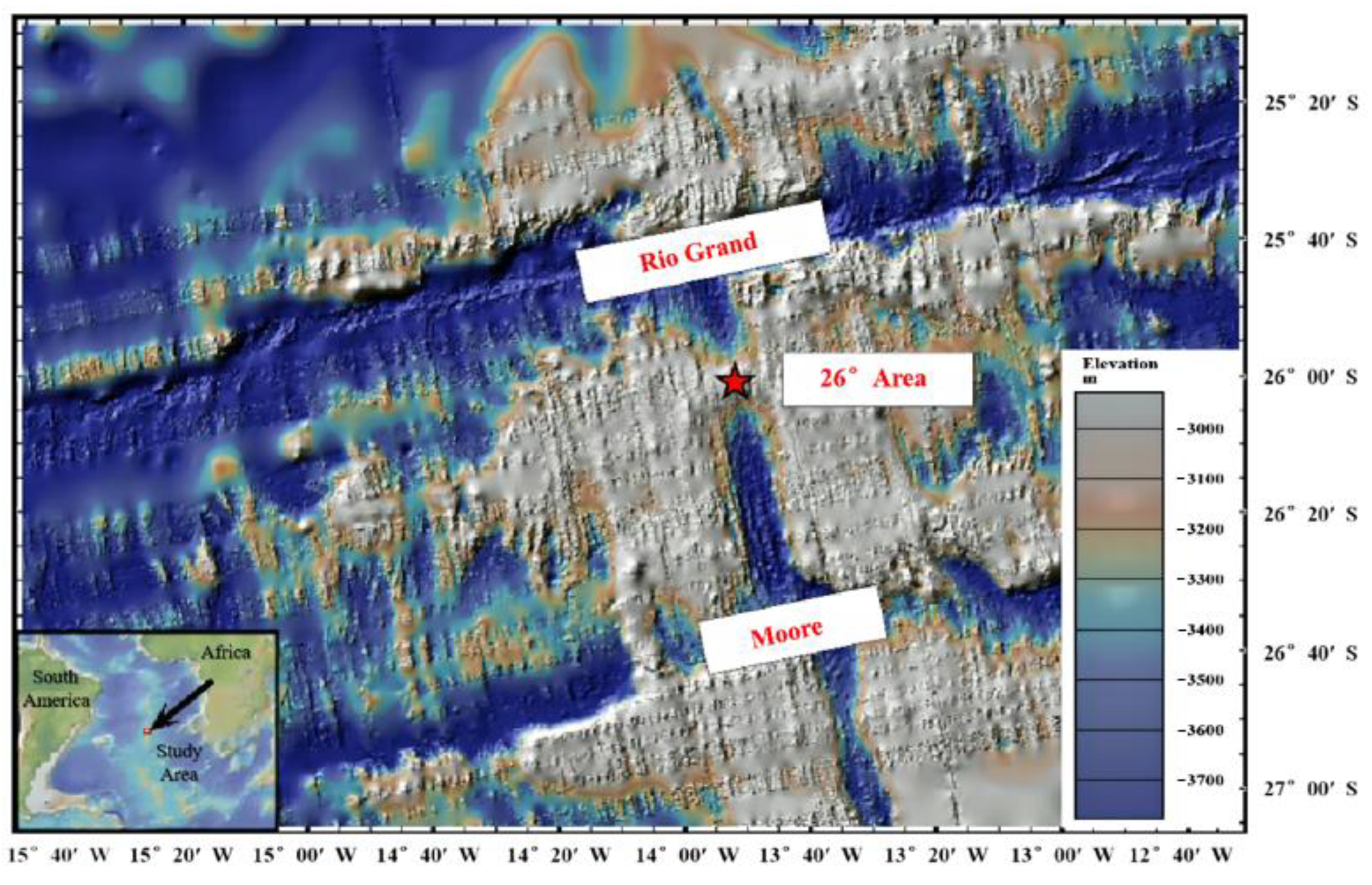
The South Mid-Atlantic Ridge is a typical slow-spreading oceanic ridge with conditions for developing large sulfide deposits [19]. As shown in Figure 1, the Austral ridge segment is located between 25°10′ S and 26°35′ S of the Mid-Atlantic Ridge [20], starts from the Rio Grand transform fault in the north, and ends at the Moore fault zone in the south, with a total length of about 100 km. The study area is located in this region. In the topographic highland of the central rift in the ridge segment, the water depth at the top is about 2600 m, and the water depth at the axial part of the transform fault is deepened to about 4100 m [21]. The area marked with a dot in Figure 1 is a typical 26° hydrothermal area called the “Xunmei hydrothermal zone”. China has surveyed hydrothermal sulfide resources in this area [22].

2.2. Data Sources

The Chinese Ocean voyage obtained several polymetallic sulfide seafloor camera data through the optical tow body in the XunMei area of the South Atlantic Ridge. The submarine camera towbody employs photoelectric composite cables to transmit electrical energy and signals to the survey ship. The system is equipped with hydrothermal anomaly detection on the camera towbody and includes an imaging unit, auxiliary light source, and bottom altimeter. Figure 2 shows the sensor and USBL. During the detection of the camera towbody, the survey vessel equipped with Global Positioning System (GPS) sailed along with the preset survey line at a constant speed of 1 to 1.5 knots in a straight line, and the camera towbody was kept 3 to 5 m from the bottom through winch operation. In order to complete the observation and video recording of the seabed situation, the seabed video image is transmitted to the scientific research vessel through the high-definition imaging unit on the tow body. The underwater positioning of the camera towbody is realized using the Posidonia 6000 USBL positioning system fixed on the drag body. The system consists of three parts: transmitting array, transponder, and receiving array. The transceiver array is installed on the ship, while the transponder is fixed on the underwater equipment to measure the underwater target position. As shown in Figure 2, the ship-borne GPS, camera equipment, and CTD (Conductivity, Temperature, Depth) work simultaneously with the USBL to detect the information of the same point. In addition, full coverage high-precision terrain data were obtained through the “Qianlong No.3” autonomous underwater vehicle (AUV, Autonomous Underwater Vehicle) at different times in the same research area.

In this study area, 28 camera survey lines were performed, and 18 were equipped with the USBL positioning system. In this case, a correction method was adopted for camera equipment for the lines with reliable USBL positioning data.

2.3. Data Analysis

The camera towbody can intuitively record and display the near-bottom video data during the detection operation in this area. Moreover, the ship-borne GPS provides the ship position data, the CTD pressure sensor obtains relatively accurate water depth data (sub-meter accuracy), and the USBL obtains the near-bottom equipment positioning information. Four kinds of equipment work simultaneously, and their information can compensate for each other’s deficiencies and cooperate to process and analyze. The accuracy of the AUV terrain data operating in the same space at different times is 1 m, which provides comparable background data for the above detection data, and provides the basis for anomaly analysis, correction, and comparison for CTD sounding data and USBL positioning data.

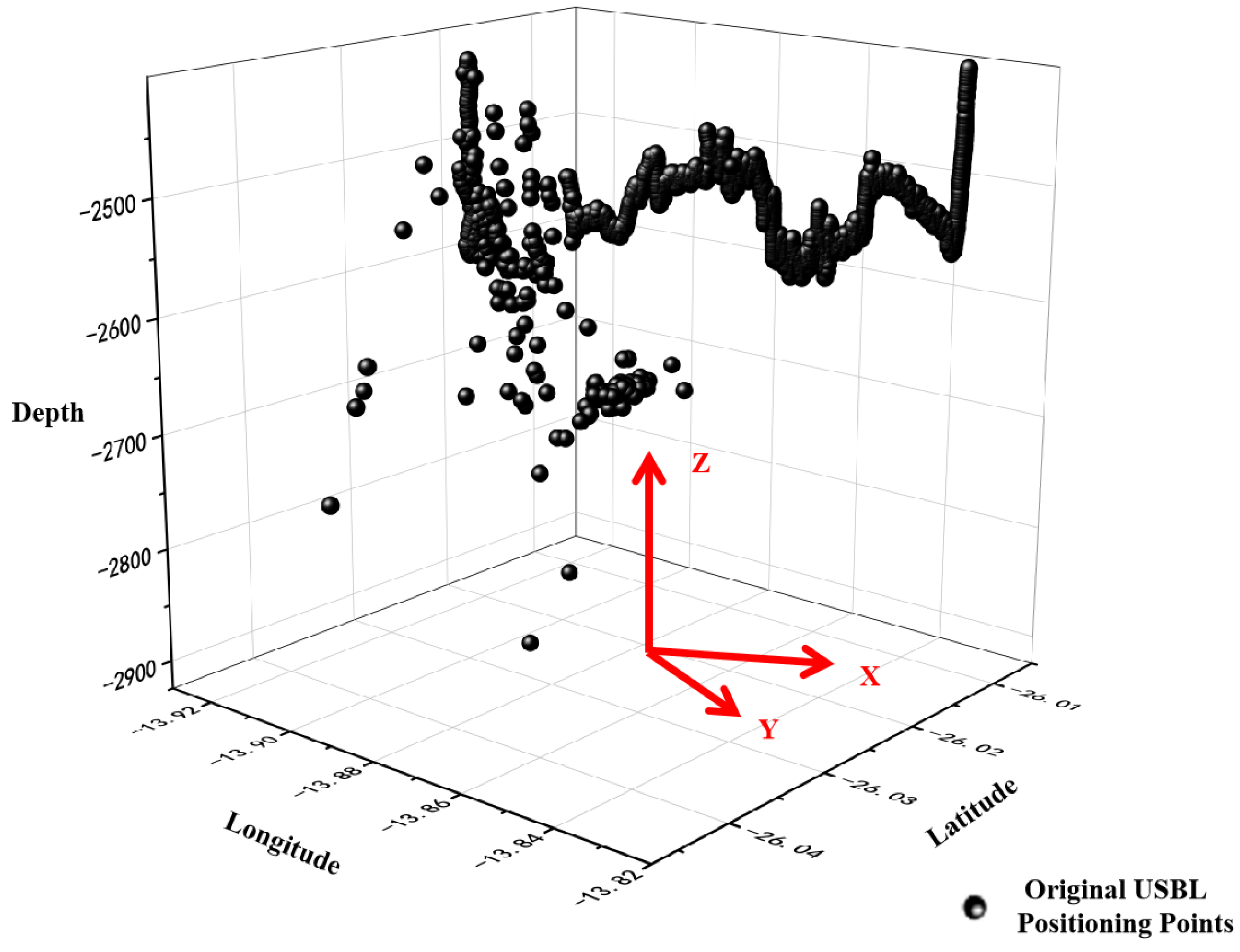
Figure 3 shows the spatial distribution of the USBL data, which contain time, longitude, latitude, and water depth data.

As shown in Figure 4, the position data of the USBL is oscillating and unstable, especially in the equipment descent process. At the beginning of the line measurement, the acquired signal is extremely unstable and generates more anomalies. The data acquired by the USBL device are more disparate and have many outliers compared with the data acquired by the CTD and other devices.

As presented in Figure 4a, the thick line is the “USBL position-CTD depth” profile of the camera survey line “2-3” of voyage 46, while the thin line is the “USBL position -USBL depth” profile. The difference between the two measurements of bathymetric data is highly significant. The CTD equipment’s detection principle and technical method are mature, and sub-meter depth data can be obtained through pressure sensors.

Regarding the comparison between the AUV and CTD depth data, as shown in Figure 4b, the dark line is the profile of “ship position-of camera depth” (water depth data from CTD, position data from shipborne GPS) of the “2-13” camera survey line, and the gray line is the water depth profile of AUV acquired in voyage 52 (water depth data from AUV, position data from USBL positioning system), whose position is compatible with the original USBL position of the “2-13” camera line, and is thus called camera equipment original position-AUV terrain profile. The two profiles maintain the same trend and morphological consistency. However, there are differences in details due to the instabilities and anomalies in the spatial distribution of the USBL positioning data. During the detection process, the stability of the operation state of the ship and equipment is preserved. Therefore, the micro-anomalies in the profile morphology caused by the instability of the USBL positioning data can be determined based on the differences between the two profiles. Accordingly, the anomalies from the USBL data in the camera line’s vertical direction(Y) can be rejected.

Figure 4c shows the USBL positioning data connected in chronological order in the ship’s direction of the “2-13” camera line, indicating that the anomalous data in the heading should not be neglected. Figure 4d shows the distribution of the USBL positioning points in the vertical ship’s travel direction(Y) of the “2-13” camera line.

The above analysis shows the necessity of analytical processing and anomaly elimination of the USBL data so they can be positioned for the camera equipment and its acquired data. Further, it is possible to eliminate its anomalies in the longitudinal direction using the CTD-detected bathymetry and the AUV terrain data and eliminate its anomalies in the navigation direction by using the GPS navigation positioning data.

3. Methods

Two key problems should be addressed to solve the positioning problem of near-bottom camera equipment and its data: (a) eliminating the USBL abnormal data employed for camera equipment positioning and (b) performing the positioning correction of camera equipment based on the USBL positioning data after abnormal processing. In order to achieve the above objectives, this paper first established a four-dimensional anomaly elimination model based on the USBL positioning data, supplemented with AUV terrain, pressure sensor bathymetry, shipboard GPS, and other data, and then established a positioning correction model for camera positioning correction. The technical flow chart is shown in Figure 5, and the specific steps are as follows.

3.1. 4D Anomaly Elimination Model

The ArcGIS10.2 technical environment and Python3.7 were employed to realize data processing and anomaly elimination, and a 4D anomaly elimination model was established. The time series (T), heading (X), vertical heading (Y), and longitudinal (Z) are the four dimensions of the 4D model. The Technology Roadmap is shown in Figure 6.

Firstly, ArcGIS was utilized to generate an “shp” graphic file from the USBL data and to judge the positioning point’s water depth and time change. The operational situation of the USBL equipment was comprehensively judged through data analysis, and then the unstable data of the USBL equipment in the descending and ascending process were removed in ArcGIS.

(1)

The USBL data obtained in (1) were correlated to the CTD data through the detection time to obtain more accurate water depth data for the USBL positioning data.

(2)

“USBL position-USBL depth” and “USBL position-CTD depth” profiles were constructed, the differences between the two datasets were compared and analyzed, longitudinal (Z) anomalies were removed using ArcGIS, and a Z-directional anomaly removal model was established.

(3)

The data in (2) were integrated with the shipboard GPS positioning data according to time and reorganized to form a new dataset.

(4)

The sequential change curve of the ship’s travel direction (X) location points was constructed based on the time series (T) in (4), as shown in Figure 4c, and anomaly clearance thresholds were developed to clear the X-direction anomaly regarding GPS time and travel progress length, and the method model was established in ArcGIS.

(5)

According to the characteristics of the USBL equipment, the water depth of the operating area, and other environmental characteristics, 0.3% of the average cable length of each measurement line of USBL was set as the initial determination threshold to eliminate the anomalous values in the vertical boat direction (Y), and a method model was established based on Python 3.7 and ArcGIS (10.2).

(6)

A “GPS position-USBL depth (CTD depth)” profile was constructed based on (4), the AUV depth was extracted based on the USBL position data in (4), and a “USBL position-AUV depth” profile was established.

(7)

The abnormal data in the Y direction (vertical survey line) were eliminated by comparing the two profiles from (7).

ArcToolbox tool of ArcGIS modeled the above data processing and anomaly-eliminating processes and methods. The location data after anomaly removal are called “restructured data”.

3.2. Positioning Correction Model

After eliminating the abnormality by the four-dimensional culling model, there will still be anomalies, and some positioning points cannot represent the position of the submarine camera, and the error is significant. Moreover, the data density of ultra-short baselines will be significantly reduced after the mentioned elimination, especially in locations with poor signal quality, qualified positioning data will be sparse or missing, and further models should be established for positioning prediction.

In order to establish the positioning correction model, several methods were employed and evaluated, including Exponential approximation, Fourier approximation, Gaussian approximation, Smoothing Spline, Kalman filtering, and Cubic polynomial least square fitting. Various fitting times were tested for each method, and the best fitting results are listed in

Table 1. The best fitting results of different methods.

Method	Degree	SSE	R-Square	RMSE
Exponential	2	0.1	0.99	0.002
Fourier	3	0.3	0.96	0.001
Gaussian	3	0	0.97	0
Smoothing Spline	default	0.1	0.97	0.001
Kalman filtering	default	0.1	0.99	0.001
Cubic polynomial least square fitting	3	0	0.99	0

.

Comparing the results in Table 1 indicates that the Cubic polynomial least squares fitting provides a zero SSE and RMSE, while the R-square is close to 1. This model is the most suitable for the construction of the correction model.

3.2.1. Polynomial Fitting Algorithm

According to the kinematics principle, the trajectory of the USBL positioning data should be a linear curve. Therefore, a specific polynomial function is proposed to fit the relationship curve.

The polynomial data fitting algorithm is as follows:

$$f\left(x\right)=p_0+p_{1}x+p_2{x}^2+\dots +p_m{x}^m$$

(1)

where $n$ data points $\left(x_i,y_i\right), i=1,2,\dots ,n$ are fitted to find $p_0,p_1,\dots ,p_m$. Based on the multiple linear regression theory, the following matrix equation can be written:$X^{T}XB=X^{T}Y$, where:

$$X=\left[\begin{array}{ccccc}1& x_1& x_1^2& \dots & x_1^m\\ 1& x_2& x_2^2& \dots & x_2^m\\ ⋮& ⋮& ⋮& \dots & ⋮\\ 1& x_n& x_n^2& \dots & x_n^m\end{array}\right]$$

(2)

$$Y=\left[\begin{array}{c}{y}_1\\ y_2\\ ⋮\\ y_n\end{array}\right] B=\left[\begin{array}{c}{p}_0\\ p_1\\ ⋮\\ p_n\end{array}\right]$$

(3)

Consider that $X^T$ is the transpose matrix of X. Let $A=X^{T}X,C=X^{T}Y$, then the problem is transformed into the linear system of equations $AB=C$. The actual data situation determines the degree m of the polynomial and the number of data points $n$. After obtaining the required model, the actual measured data are compared with the theoretical one obtained by the formula to calculate the error to measure the fitting quality; that is, appropriate parameters are chosen to make the fitting function. The mean square error with the actual observed value $\mathrm{R}={\displaystyle \sum }_{\dot{i}=1}^m{\left(\phi \left(x_i\right)-y_i\right)}^2$ reaches the minimum, and the obtained curve is called the fitting in the sense of the least-square method [23].

3.2.2. Polynomial Least-Squares

Appropriate parameters are selected to minimize the mean square error between the fitting function and the actual observed value. At this time, the obtained curve is called the fitting curve in the sense of the least-squares method. In order to evaluate the fitting accuracy, SSE, R-square, and RMSE are employed.

$$\mathrm{SSE}={{\displaystyle \sum }}_{i=1}^n{w}_i{\left(y_i-\widehat{y_i}\right)}^2$$

(4)

$$\mathrm{RMSE}=\sqrt{\mathrm{SSE}/n}=\sqrt{\frac{1}{n}{{\displaystyle \sum }}_{i=1}^n{w}_i{\left(y_i-\widehat{y_i}\right)}^2}$$

(5)

where $y_i$ and ${\widehat{y}}_i$ represent the actual and fitted data, respectively. SSE calculates the sum of squares of the errors between the fitted data and the corresponding points of the original data. RMSE describes the root mean square error between the predicted and original data.

The closer the SSE and RMSE are to 0, the better the model fitting effect is.

$$\mathrm{SSR}={{\displaystyle \sum }}_{i=1}^n{w}_i{\left(\widehat{y_i}-\overline{y_i}\right)}^2$$

(6)

$$\mathrm{SST}={{\displaystyle \sum }}_{i=1}^n{w}_i{\left(y_i-\overline{y_i}\right)}^2$$

(7)

$$\mathrm{R}-\mathrm{square}=\frac{\mathrm{SSR}}{\mathrm{SST}}=\frac{\mathrm{SST}-\mathrm{SSE}}{\mathrm{SST}}=1-\frac{\mathrm{SSE}}{\mathrm{SST}}$$

(8)

SSR is the sum of squares of the difference between the fitted data and the mean of the original data. SST is the sum of squares of the difference between the original data and the mean. The “coefficient of determination” (R-square) is defined as the ratio of SSR to SST, and the closer the value is to 1, the better the model fits the data.

3.3. Camera Positioning Correction

This paper implements the Cubic Least square fitting method by MATLAB(R2016Bb). Moreover, the positioning correction model of the measuring line is established based on “restructured data” from 3.1, which is a time series as the index. The steps are as follows:

(1)

Using the method implemented by MATLAB, the “restructured data” is substituted into the polynomial Equation (1), and simulated by varying the value of m from 1 to 5, to compare and judge the three indicators of SSE (summed variance), R-square (coefficient of determination) and RMSE (fitted standard deviation).

(2)

When the SSE and RMSE values are close to 0, R-square is close to 1 and tends to be smooth while increasing m. Now, the value of m is taken as the highest number of polynomials or the number of final correction models.

(3)

In order to ensure robustness, the data are centralized and normalized using the conventional least squares, and their correction coefficients are calculated using the data number (time order) as x and the longitude or latitude as f(x), respectively, to fit the USBL data. A 95% confidence interval fitting constant indicates that the data and method are satisfactory.

(4)

The calibration model qualified for testing and training is employed to simulate the USBL positioning data with the removed exceptions, and interpolation prediction is performed according to the required video positioning accuracy to obtain near-bottom video positioning.

4. Application

The implementation of the proposed method is divided into four parts: eliminating anomalies with a four-dimensional model, constructing the correction model, positioning correction of video data, and verifying the application results.

4.1. Anomaly Elimination

Helpful information is extracted from the USBL positioning data obtained in the field, and a four-dimensional culling model is established for the time series (T), heading (X), vertical heading (Y), and longitudinal direction (Z), as shown in Figure 3. X represents the distance of the USBL points along with the heading direction, Y represents the distance of the USBL points in the vertical direction of the heading, and Z represents the vertical distance of the USBL points. Z describes the water depth value as the first judgment basis, which is less disturbed. Since there may be many abnormal points in different periods in the X direction, which fall in the dense area of another period, the elimination is not performed entirely, which creates difficulties for the judgment of the X direction. Therefore, Y is adopted as the second judgment object, while the X direction performs the auxiliary judgment. As long as one of the X, Y, and Z directions is abnormal, it is defined as locating abnormal data and is eliminated.

4.1.1. Eliminating Outliers in the Z Direction

In the Z direction, many points with obviously abnormal water depth can be seen after arranging the USBL data of a survey line in chronological order. Firstly, obvious outliers were removed during the descent and ascent of the USBL device, and the remaining positioning data were kept as the initial dataset. Since the positioning data are acquired in 1 s on average, the data sequence of the measuring line is taken as a segment every 10 s (the distance that the boat travels at this time is about 5 m), and the abnormal water depth value in each segment is statistically determined, and the data point is eliminated when the deviation exceeds 10 m.

Taking the black dotted line circled in Figure 7a as an example, the red points deviate from the normal water depth value and have a very low distribution density. These data are the points with obviously abnormal water depth values, while the data of points with similar distribution status that deviate from the reasonable water depth values are excluded.

This problem can also be solved by performing a linear simulation of the data, as shown in Figure 7b, and a moving average of the data was employed to obtain a simulated curve. Outliers with simulation residuals above 10 m are removed to obtain a dataset with preliminary clearance of anomalies.

Moreover, the above dataset can establish a “USBL position-USBL depth” profile. Furthermore, the dataset can be associated with the CTD data through the time field, and a “USBL position-CTD depth” profile is constructed using the USBL position and CTD depth in the same position and time, as shown in Figure 4a. The “USBL position-USBL depth” profile is compared with the “USBL position-CTD depth” profile, and the USBL data are eliminated for points or areas whose bathymetry trends differ significantly.

4.1.2. Eliminating Outliers in the Y Direction

After removing the Z direction, the USBL still has many outliers in the two-dimensional angle of latitude and longitude. Buffers are constructed in the vertical direction of clustered, trended, and reliable drag body position data. Since the USBL array is calibrated, the positioning accuracy must be within 0.3% of the slant range [24]. Therefore, the buffer zone range is set as 0.3% of the average length of each measuring cable.

The “Buffer” method from ArcGIS was employed to establish a model, which sets the “Average Length (m) × 0.3%” as the buffer radius to eliminate the preliminary anomalies of the Y-direction of the target measurement line.

After eliminating the points outside the buffer, the remaining data have a better positioning quality, as shown in Figure 8.

As shown in Figure 8, the red points are the more credible drag points after being eliminated by the blue buffer, and the data outside the blue area are the abnormal data, which will be eliminated.

The GPS data and the above USBL dataset were associated with the time field. Then, a “GPS position-USBL depth (CTD depth)” profile is established using the GPS position and USBL depth (CTD depth) at the same time and position.

ArcGIS employs the method of the “Extract attribute by points” raster data tool to extract AUV depth data with the above USBL points positions. Then, a “USBL position-AUV depth” profile is constructed, as shown in Figure 4b.

The “GPS position-USBL depth (CTD depth)” profile is compared with the “USBL position -AUV depth” profile. The USBL localization points in the areas of the “USBL position -AUV depth” profile with significant morphological variations are eliminated.

This completes the Y-direction (vertical survey line) anomaly elimination.

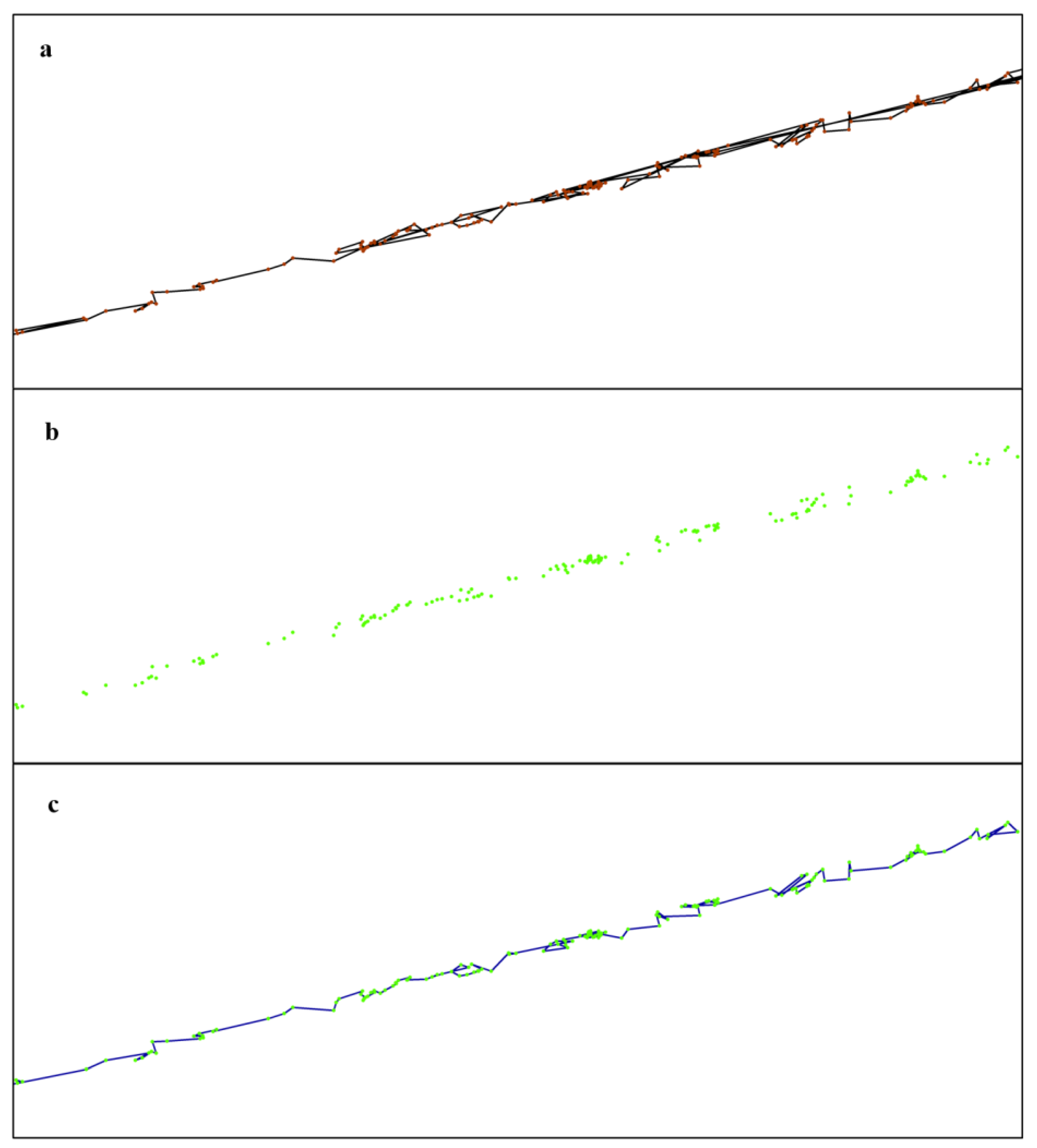
4.1.3. Eliminating Outliers in the Time and X Direction

The datasets obtained after eliminating the anomalies in the Z and Y directions are still the new “restructured data”. At this point, the “restructured data” are arranged in time sequence, plotted in ArcGIS, and sequentially connected into lines. Then, the analysis of their distribution characteristics in the time series in the X-direction indicated that with the increase in time T, the distribution of folding lines was not sequentially arranged on a curve according to the trend but backward and forward, as shown in Figure 9a. It demonstrates the existence of anomalies, and the anomalous data in the X-direction should be eliminated based on time T.

Since the ship and the underwater detection equipment simultaneously traveled along the same course, they maintained the same speed and position. In order to obtain the range of possible changes in USBL positioning points, the changes in GPS positioning points and position are calculated simultaneously. For example, if the GPS line corresponding to the “2-13” camera line and the USBL measurement line traveled within 1 to 5 m in an average of 5 s, the maximum travel speed of the measurement line equipment was 1 m/s. Thus, the distance of the USBL measurement line cannot exceed 1 m in 1 s. The distance of the measurement point within 1 s adjacent to the USBL positioning point cannot exceed 1 m, and a distance of more than 1 m is regarded as an anomaly. The distance of adjacent positioning points can be calculated using Equation (9). The positioning points whose distance exceeds 1 m in 1 s are eliminated. Accordingly, the abnormal data in the X direction and T sequence is eliminated. This leads to positioning datasets with eliminated anomalies in the X direction.

D_i = (T_{i + 1} − T_i) × 1 m/s

(9)

where Di is the distance from the point i to point i + 1 in the sorted reconstituted dataset, T is the detection time of the locating point, and 1 m/s is the travel speed of the equipment acquired from GPS.

This operation was performed in ArcGIS. Due to the instability of USBL equipment operating underwater, the upper threshold of the distance traveled per second is set to 3 m. The dataset was generated as a vector layer according to the time series, the point series was connected to a polyline, and the length of its sections was calculated. If D_i/(T_{i + 1} − T_i) > 3 m/s, the data were considered abnormal, and the point was eliminated. Accordingly, the anomalies in the X-direction and T sequence of the camera line “2-13” were eliminated, and a new dataset was obtained after 4D anomaly elimination, as shown in Figure 9b,c.

After the above operation, the 4D anomalies are eliminated from the USBL data. Now, the model data are ready for simulation. The green dot in Figure 10 indicates the “restructured data” of the camera line “2-13” obtained after eliminating the corresponding USBL anomalies.

4.2. Correction Model

Camera positioning correction can be realized based on the datasets obtained in Section 4.1.3 after 4D anomaly elimination. Taking the dataset of the camera survey line “2-13” with 12,200 points as the model data, the polynomial least-squares fitting method is employed to fit and correct it. As shown in Table 1, the three index parameters are compared for m = 1, …, 5.

It can be seen from

Table 2. Comparing the fitting performance indices for different values of m.

m	SSE	R-Square	RMSE
1	0.1	0.94	0.003
2	0.4	0.97	0.002
3	0	0.99	0
4	0	0.99	0
5	0	0.99	0

that the fitting effect becomes better by increasing the value of m. When m = 3, the SSE and RMSE values are close to 0, and the R-square is close to 1. When m exceeds 3 (m = 4, 5), the fitting performance indices are kept unchanged. Therefore, m = 3 is suitable for fitting and correcting USBL data. Accordingly, the following polynomial function is chosen for the data fitting.

$$f\left(x\right)=p_0+p_{1}x+p_2{x}^2+p_3{x}^3$$

(10)

Therefore, the cubic polynomial least-squares method is adopted to establish the fitting model, as shown in the above formula, with the serial number (time sequence) as $x$ and the longitude and latitude as $f\left(x\right)$. After centralization and standardization, the correction coefficients were calculated, and the currently available USBL data were fitted and corrected to obtain the fitting constant within the 95% confidence interval. These fitting constants are substituted into Equation (9) to obtain the fitting curve equation and establish the fitting model.

4.3. Camera Positioning

4.3.1. Location Model Simulation

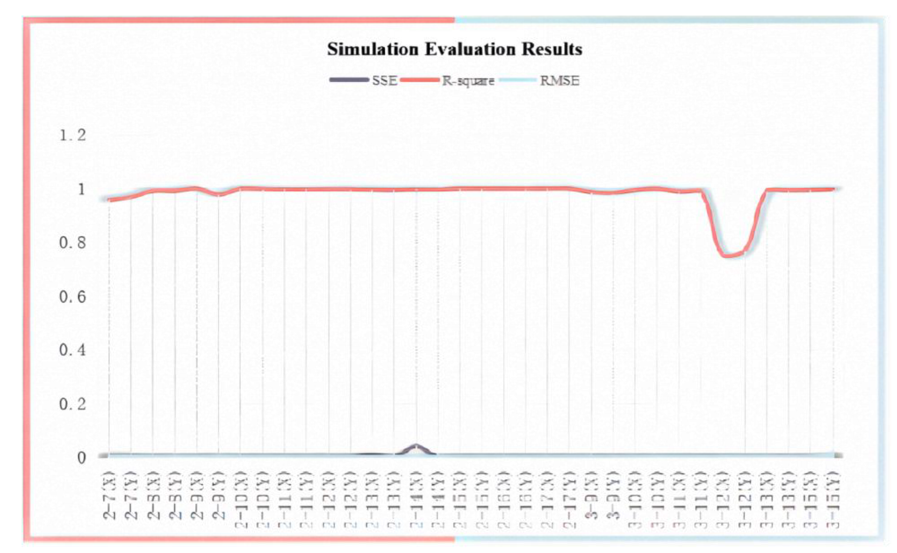
After eliminating the 4D abnormality, the corresponding USBL data of the camera line were selected, and the mentioned correction model was adopted to simulate the USBL positioning data.

The fitting effect is evaluated using the above three parameters (mentioned in Section 3.2.2). The results are shown in Figure 11.

As shown in Figure 11, the simulation results indicate that the number of lines with SSE and RMSE less than 0.01 accounts for about 85%, and the number of lines with R-square between 0.9 and 1 accounts for about 95%, indicating the high fitting accuracy of the proposed method. Among them, the determination coefficient of the camera survey line “3-12” is about 0.75 due to the severe shortage of qualified data for the line, which also shows that the proposed method is unsuitable for correction for the USBL data with poor quality.

The simulation results show that the above methods and procedures are suitable for calibrating all camera lines except for the case of the “3-12” line.

4.3.2. Positioning for Camera

The positioning correction can be performed for the camera based on the corresponding USBL data sequence that has passed the correction model test in the mentioned positioning model simulation.

The “restructured data” eliminated by the 4D anomaly elimination model and sorted in time series are taken as the model data and substituted into Equation (10) to obtain the corrected model curve through simulations. Then, the continuous-time simulated positioning data are obtained based on the fitted curve equation. The curve equation is employed for camera positioning correction. Taking the time series dataset of the “2-13” camera line as an example, the above 12,200 data are employed to train and simulate the correction model. Accordingly, the positioning correction curve equation is obtained. Then, according to the camera positioning point density requirements, 1 s is taken and substituted into the curve equation. Then, the sequence of longitude and latitude coordinate pairs corresponding to f(x) in the equation of the 1-s interval is obtained, which gives the camera positioning data of the 1-s interval. Figure 12 shows the distribution of the camera line after positioning. The yellow point indicates the position after the simulation correction of the USBL (camera position), and the green point indicates the predicted camera position.

4.3.3. Correction Result

The accurate and fast positioning of the camera and its data is realized under the existing conditions and the established operation mode using the above method to obtain the submarine camera’s geographic location. Figure 12 and Figure 13 show the effect of the “2-13” camera line correction and positioning. After the correction, the position of the underwater camera becomes continuous and stable from the longitude, latitude, and water depth values.

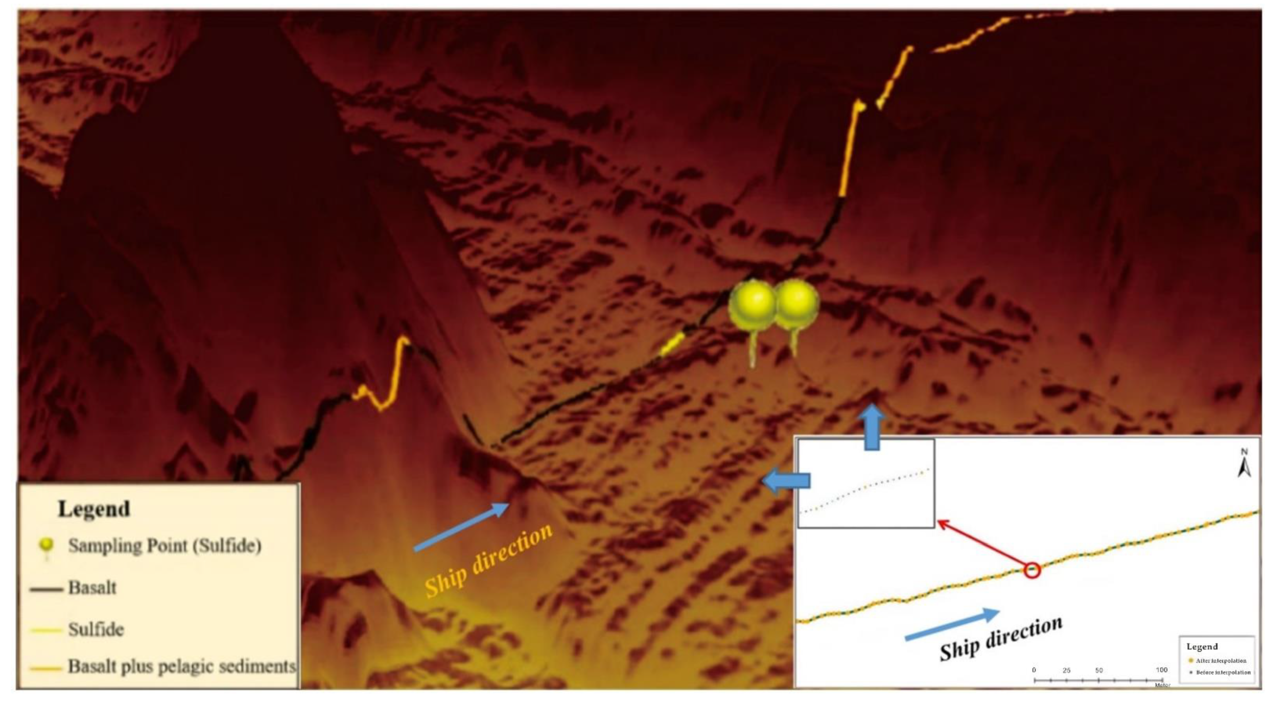
As shown in Figure 14, the “2-13” camera survey line’s water depth profile after positioning correction is highly compatible with the AUV terrain. After the camera positioning correction, the substrate type interpreted according to the video corresponds to the two TV grab station’s sample types in the same location.

This work corrects the USBL positioning data of 17 camera lines. All camera points of each line are positioned according to the accuracy requirement. The principle of de-isotropy and fidelity was followed while removing anomalies from the original USBL positioning data of the camera lines to provide high-quality model data for establishing the correction model, optimizing the correction model, and ensuring the accuracy of the correction results. The positions after correction and prediction are reasonably compared with the GPS positioning data. The sample types acquired from the geological sampling points are consistent with those identified by the camera data at the same positions obtained by correcting and predicting. After positioning, the depth profiles of the 17 camera lines are compatible with the AUV terrain and fit perfectly. Accordingly, the subsequent use of the camera data was ensured.

5. Discussion

The USBL positioning equipment signal is relatively stable in flat seabed terrain. However, there may be multipath effects in areas with complex terrain, degrading signal tracking and causing unstable positioning data. Due to the positioning anomalies caused by various factors, such as terrain, bottom current, weather conditions, and equipment, the USBL positioning data cannot guarantee an accurate and practical indication of the position of the underwater camera. Therefore, some processing and corrections are required to solve the positioning problem of submarine camera data.

The seabed camera trajectory is linear. The simulation of linear feature data implies eliminating as much anomalous data as possible to ensure the effectiveness of the simulation. This paper establishes a four-dimensional anomaly elimination model based on time and space sequences, eliminates the USBL anomalous data, and provides reliable model data for establishing the correction model. This is the most critical step in all similar calibration and simulation works for the USBL data and is also the key to achieving better results in this paper.

This paper evaluates various commonly-used linear models, selects the best polynomial least squares method to simulate the localization data, and determines the cubic polynomial least squares method as the most suitable model. The screening and testing of the method can provide a reliable basis for further localization correction.

This paper adopts the USBL positioning data, combined with the pressure sensor bathymetric data bound to the drag body, the AUV high-precision terrain data, and the shipboard GPS positioning data to establish a four-dimensional abnormal elimination model from the time and space scales, to eliminate abnormal data generated by changes in heading, vertical heading, depth direction, and travel time T of the USBL data. This is an unprecedented innovation in thinking, which guarantees future relevant work.

In order to evaluate the effectiveness of the proposed method, the 5000 USBL positioning points with good positioning quality were randomly selected uniformly from the “restructured data” of the “2-13” camera survey line without participating in the model simulation, marked according to the time sequence, and the remaining data were simulated. Then, the positions of the above 5000 points were obtained according to the fitting curve. The predicted positions were compared with the original ones, and the paired sample T-test method [25,26] was employed to evaluate the difference between the data after fitting and the original positioning data. The test results are shown in

Table 3. Comparing the Data Before and After Positioning.

Pair	Cases	Correlation	Salience
Longitude	5000	1	0
Latitude	5000	1	0

.

After comparison, when the confidence interval is 95%, the correlation coefficient is 1, and the significance is 0, indicating no significant difference between the processed and original positioning data. Moreover, the error range between the predicted positioning data and the original one is within 5 m, which is within an acceptable range for the current seabed survey and positioning technology level.

After processing the experimental data with the USBL positioning data method in [13,15], it is found that the processing results of this paper are significantly superior to the literature because the previous studies were confined to only ultra-short baselines. The positioning data are analyzed and processed. Various errors in the ultra-short baseline data generally lead to limitations, affecting the calibration results’ accuracy. However, this paper not only eliminates and corrects the erroneous data generated by the change of the heading along with the travel time, that is, the time factor but also combines the necessary various related data to perform the positioning correction. This shows that the proposed ultra-short baseline positioning data, supplemented by a comprehensive analysis of other relevant data, can effectively solve the inaccurate spatial positioning of underwater cameras.

6. Conclusions

This paper solved the problem of positioning for deep-sea near-bottom camera data. Firstly, the ultra-short baseline(USBL) positioning data, ship-borne GPS positioning data, pressure sensor bathymetric data, and AUV terrain data were analyzed and mined comprehensively in ArcGIS. Secondly, a four-dimensional elimination model was established based on time series (T) and space series (X, Y, Z) to eliminate abnormal data, including the abnormal data generated on the direction of the ship (X), the Vertical X (Y), the vertical direction (Z), and the time series (T). Thirdly, a cubic polynomial least-squares correction model is established for correcting the position of the camera data.

The model was applicated to the data collected in Xunmei. Its SSE and RMSE values are close to 0, the R-square is close to 1, and the fitting constants are within 95%. In those corrected data, the data with variance and fitting standard deviation less than 0.01 accounted for about 95%, and the data with determination coefficients between 0.9 and 1 accounted for about 95%. Accordingly, the fitting accuracy of this method is high, meaning that it is suitable for fitting USBL data and positioning camera data.

After positioning correction, the position of the camera survey line is highly compatible with the AUV terrain. The water depth profile of the camera survey line is compatible with the topographic trend. The type of substrate interpreted from the video data is compatible with the sample type sampled by the TV grab bucket in the same location. No significant difference can be observed between the predicted positioning data and the original data in the area with high-reliability USBL signals, and the error range of the predicted position through model simulations is within 5 m. Thus, the feasibility and reliability of the proposed method for locating and correcting near-bottom camera data are verified. Therefore, this method can be utilized in production practice. This paper established a foundation to form the corresponding processing software to achieve efficient processing in field operations in the future.