Article

Prediction of Prospecting Target Based on Selective Transfer Network

1
Faculty of Intelligent Manufacturing, Wuyi University, Jiangmen 529000, China
2
State Key Laboratory of Public Big Data, Guizhou University, Guiyang 550025, China
3
College of Computer Science and Technology, Nanjing University of Aeronautics and Astronautics, Nanjing 210016, China
4
College of Computer Science and Technology, Nanjing Forestry University, Nanjing 210095, China
*
Author to whom correspondence should be addressed.
These authors contributed equally to this work.
Minerals 2022, 12(9), 1112; https://doi.org/10.3390/min12091112
Submission received: 25 July 2022 / Revised: 20 August 2022 / Accepted: 27 August 2022 / Published: 31 August 2022

Abstract

:
In recent years, with the integration and development of artificial intelligence technology and geology, traditional geological prospecting has begun to change to intelligent prospecting. Intelligent prospecting mainly uses machine learning technology to predict the prospecting target area by mining the correlation between geological variables and metallogenic characteristics, which usually requires a large amount of data for training. However, there are some problems in the actual research, such as fewer geological sample data and irregular mining features, which affect the accuracy and reliability of intelligent prospecting prediction. Taking the Pangxidong study area in Guangdong Province as an example, this paper proposes a deep learning framework (SKT) for prospecting target prediction based on selective knowledge transfer and carries out intelligent prospecting target prediction research based on geochemical data in Pangxidong. The irregular features of different scales in the mining area are captured by dilation convolution, and the weight parameters of the source network are selectively transferred to different target networks for training, so as to increase the generalization performance of the model. A large number of experimental results show that this method has obvious advantages over other state-of-the-art methods in the prediction of prospecting target areas, and the prediction effect in the samples with mines is greatly improved, which can effectively alleviate the problems of a small number of geological samples and irregular features of mining areas in prospecting prediction.

1. Introduction

Mineral resources are an essential strategic resource to ensure national stability and economic development. After years of geological exploration, surface minerals have gradually become scarce, resulting in a further increase in the difficulty of prospecting. The prospecting work started in deep surfaces and overburdened areas. In recent years, the development of machine learning technologies, especially deep learning, has achieved satisfactory success in many fields, e.g., in computer vision [1], natural language processing [2], synthetic aperture radar [3], and atmospheric prediction [4]. Meanwhile, it has also interested and been selected by geological researchers [5,6,7,8]. Therefore, the traditional geological prospecting method is gradually turning into an intelligent prospecting method based on machine learning.
An intelligent prospecting target refers to the use of machine learning technologies to mine the correlation between geological variables and metallogenic characteristics to predict the metallogenic target area [9,10]. Although quantitative prospecting target prediction based on machine learning technologies is in its infancy, some progress has been made. These works can be divided into the following three categories according to the method of implementation:
(1)
Methods based on ensemble learning combine multiple supervised learning algorithms for prospecting target prediction. For example, the authors in [11] determined the hyperparameters of the random forest by simulating the natural evolution process, which were used to improve the accuracy of the model in predicting the prospecting target area. The authors in [12] used the isolation forest algorithm to predict outliers to determine the prospecting target area. The authors in [13] proposed the use of metric learning in the random forest to project the sample features into the feature space, separating the background and mining targets, so as to improve the prediction accuracy of the model.
(2)
Methods based on the support vector machine (SVM) divide mining samples and other samples through a hyperplane. For example, the authors in [14] separated the “mines” samples from “non-mines” samples through the optimal hyperplane and determined three prospecting target areas on both sides of the hyperplane. The authors in [15] used a genetic algorithm to optimize the hyperparameters of SVM to reduce its influence on prospecting target prediction.
(3)
Methods based on depth neural networks project the geoscience data into the same depth neural network space and extract effective features through multiple nonlinear transformations for prospecting target prediction. For example, the authors in [16] used three-layer convolution to extract the features of a Zn-element concentration distribution map to predict the prospecting target area. The authors in [17] used AlexNet to extract the features of multiple ore-forming factor maps to determine four prospecting target areas.
Although the aforementioned methods have achieved success, problems such as the small number of geological samples and the irregular features of mining areas in prospecting target prediction have not been properly solved. Fortunately, in recent years, in-depth research has been carried out on these problems. These works can also be divided into the following two categories according to the method of implementation:
(1)
Methods based on data augmentation increase the diversity of geological samples by cropping, changing the chromatic aberration and size, and distorting features. For example, the authors in [18] added random noises into geological data to predict a prospecting target by a deep convolutional network. The authors in [19] first oversampled the samples with mines and then used the random forest to determine the prospecting target areas. The authors in [20] proposed recombining pixel pairs of geological samples to assist in prospecting target prediction. These methods increase the number of geological samples but cannot cope with the irregular features of the mining areas.
(2)
Methods based on multiscale feature transformation acquire mining area features of different scales through irregular sampling for training [21,22]. For example, the authors in [23] proposed to extract irregular features of different scales using multigroup convolution or a pooling operation and fused them for prospecting target prediction. The authors in [24] used four convolution operations with different sizes to extract and fuse irregular features of geological data to improve the prediction accuracy. However, these methods do not consider the small number of samples in the prospecting target area.
To summarize, the motivation behind our method comes from two aspects: (1) Selective transfer of label information learned from large tasks to small-shot tasks can effectively improve its generalization performance; therefore, we try to selectively transfer knowledge from a well-trained large prospecting target prediction task to the target task to assist training. (2) The other is to expand the receptive field of the convolution kernel without increasing the number of parameters. In this way, we can utilize it to deal with the irregular features of the mining areas. Therefore, we combine these two motives and propose a novel deep learning framework based on selective knowledge transfer (SKT) for prospecting target prediction to solve the problems existing in prospecting target prediction. As shown in Figure 1, we first introduce a large well-trained prospecting target prediction network as the source network and define multiple target networks with the same structure. Next, we use a soft mask to alleviate the differences in metallogenic effects that different elements may cause. Then, we use dilated convolution to capture features of different scales as inputs of the target networks. Based on this, we selectively transfer the weight parameters from the source network for the training of the different target networks. Finally, we perform top-down distillation on the large-scale and small-scale target network to mine the hidden knowledge between feature maps of different scales for small-scale target network learning. It is worth noting that the input size of W × H × n is obtained by processing the geochemical data, where W denotes width, H denotes height, and n denotes the number of geochemical elements. Meanwhile, the output is generated by voting through all the target networks and contains two values representing the votes obtained for with and without mines, respectively. The whole SKT framework works in an end-to-end manner. Extensive experimental results show that our method is significantly competitive with state-of-the-art methods.
The main contributions of this paper include the following:
1.
A deep learning framework for prospecting target prediction is proposed, which provides a new way for prospecting target prediction.
2.
A novel selective knowledge transfer mechanism is designed, which selectively transfers knowledge from the source network to target networks, which increases the performance of the target networks in prospecting target prediction during testing without adding additional computational cost.
3.
For the first time, a soft mask strategy is proposed to maintain the consistency of related mineral elements. Its purpose is to utilize the metallogenic indicative significance of the main mineral elements and associated mineral elements to complete the prospecting target prediction task.
The rest of this paper is organized as follows. Section 2 introduces introduces the study area and data processing methods. Section 3 infers the structure of the SKT framework. Section 4 exhibits our experiment, including analysis of the experimental results and visualization. Section 5 summarizes the work of this paper.

2. Study Area and Data

2.1. Study Area

The study area is the Pangxidong study area in Guangdong Province, China. Figure 2 shows a simple geological map of the study area, where the red dots are the mining areas. It is a part of the Qinzhou–Hangzhou metallogenic system, and the metallogenic geological conditions are superior. Its tectonic background belongs to the eastern margin of the southern segment of the Qinzhou–Hangzhou metallogenic system. Since the late Paleozoic, it has been uplifted for a long time and is an important metallogenic area for precious metals and non-ferrous metals, with many kinds of minerals [25]. The minerals that have been explored or are being exploited include gold ore, silver ore, lead–zinc ore, tungsten and molybdenum ore, iron ore, etc. [26]. The types of deposits mainly include ductile shear zone silver–gold deposits, porphyry-type molybdenum–tungsten–copper polymetallic deposits, sedimentary reformation type, magmatic hydrothermal type, and contact metasomatic lead–zinc polymetallic deposits [27]. Minerals are mainly distributed in the northwest and southeast, along the Pangxitong fault zone and the Gucheng–Shachan fault zone, in a northeast direction.

2.2. Data Processing
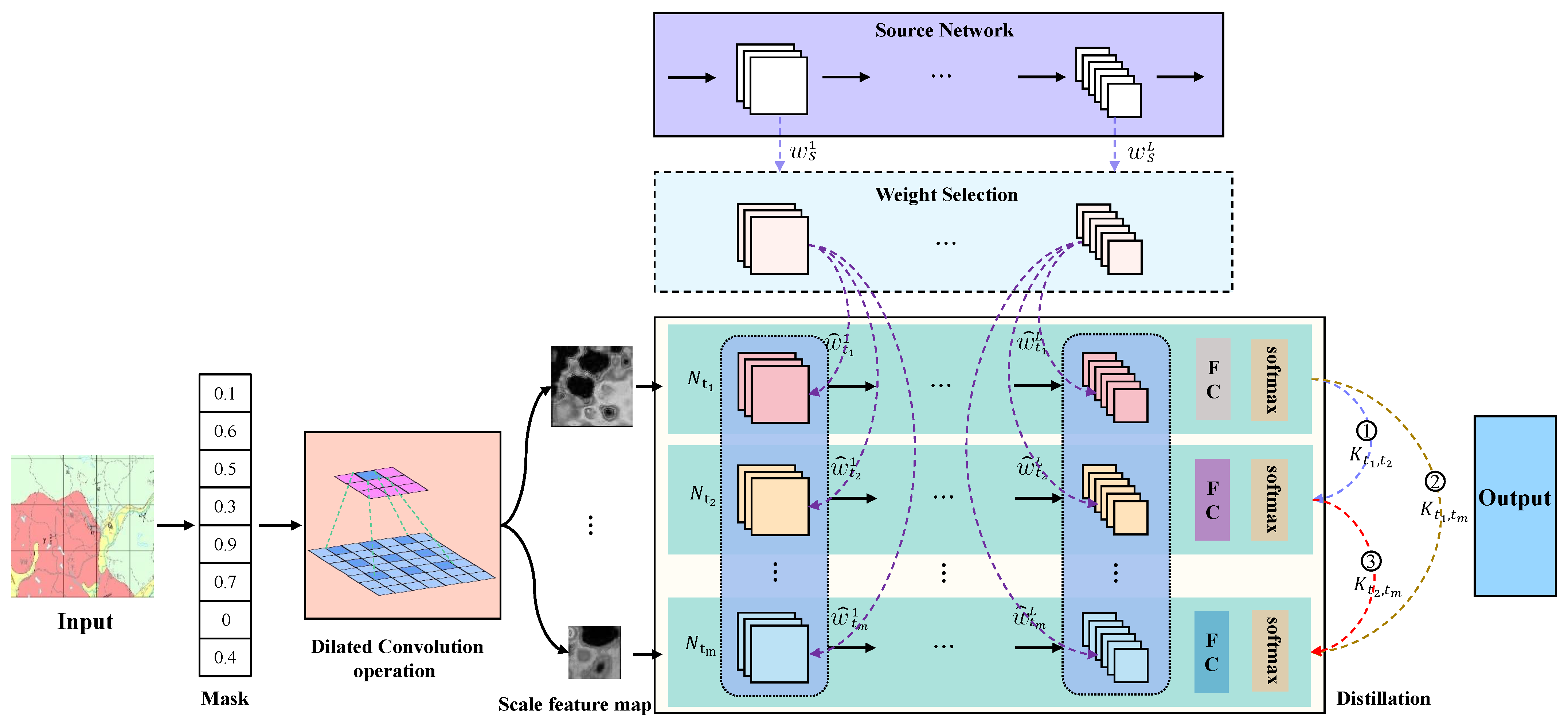
The experimental data consist of geochemical data and were extracted from a 1:50,000 stream sediment survey. They were obtained from the Pangxidong study area in Guangdong Province. The sampling area of the stream sediment was 1694 km 2 , and the average sampling density was 4.27 samples km 2 . Sixteen chemical elements, including Au, B, Sn, Cu, Ag, Ba, Mn, Pb, Zn, As, Sb, Bi, Hg, Mo, W, and F, were analyzed from the stream sediment samples. Table 1 shows some of our original data, with X and Y as the coordinates of the sampling points and the rest as the values of the geochemical elemental content, totaling to 7237 points. The area under curve (AUC) is defined as the area under the receiver operating characteristic (ROC) curve enclosed by the coordinate axes [28]. Based on thesis [29], we leveraged SVM and statistical methods to screen out geochemical elements, which are indicative of mineralization. Specifically, we calculated the AUC of each element using the SVM algorithm, and then the standard deviation of the AUC was calculated by
S AUC = AUC ( 1 AUC ) + C p 1 Q 1 AUC 2 + C n 1 Q 2 AUC 2 C p × C n
where S AUC denotes the standard deviation of the AUC; C p and C n denote the numbers of samples with and without mines, respectively; and Q 1 = AUC 2 AUC and Q 2 = 2 AUC 2 1 + AUC are temporary variables. To determine whether the AUC was significantly different from 0.5, we defined the following random variable:
Z AUC = AUC 0.5 S AUC
The random variable Z AUC satisfies a standard normal distribution. The critical value is obtained by comparing Z AUC with the standard normal distribution table. Based on Table 2, we chose a Z AUC greater than the critical value of 2.58 when the significance level was 0.01. In other words, a total of eight elements, including Au, Sn, Cu, Ag, Ba, Sb, Hg, and Mo, were selected as indicative elements for prospecting target prediction.
We combined experimental results and the geological environment of the study area for analysis. The Pangxidong study area has faults, developed fold structures, and strong magmatic activity. The metallogenic geological environment is similar to many areas with rich mineral resources in the Qinzhou–Hangzhou metallogenic belt. The types of minerals involved are mainly Au, Ag, Pb, Zn, W, Mo, Fe, and Mn metal ores. Then, Pb, Zn, and Cu metal ores are visible in Devonian strata in the study area. In addition, the northeast Gucheng–Shachan and Pangxitong faults in the study area are the main ore-conducting and storage structures for Au, Ag, Sn, and other minerals [30]. In summary, most of the eight indicator elements we selected are consistent with the metallic ores in the study area. This shows the validity of our choice of indicator elements.
By referring to the processing method of the stream sediment data in [31], we used inverse distance weight interpolation to generate 3072 × 3072 grids (elemental content map) according to the values of the geochemical elemental content. Specifically, we calculated the distance between the nearby discrete points and the grid x 0 , y 0 by
D i = x 0 x i 2 + y 0 y i 2
where D i denotes the distance from the i-th discrete point near x 0 , y 0 , and x i , y i denotes the coordinates of the i-th discrete point.
Based on this, we estimated the value of the grid x 0 , y 0 as follows:
Z x 0 , y 0 = i = 1 N 1 D i 2 Z i / i = 1 N 1 D i 2
where Z x 0 , y 0 denotes the estimated value at the grid x 0 , y 0 , Z i denotes the observed value at the i-th discrete point, and N denotes the number of discrete points involved in the calculation.
Figure 3 shows the elemental content maps of the eight elements. We normalized the values of the elemental content map, making its mean value 0 and its variance 1. For a value x in the elemental content map, the normalized value is as follows:
x ^ = x x ¯ σ
where x ^ denotes the normalized value, x ¯ denotes the mean of the values of the elemental content map, and σ denotes the variance of the values of the elemental content map.
We divided the elemental content map of size 3072 × 3072 into two parts, where the upper part (2560 × 3072) was used for making the training dataset, and the lower part (512 × 3072) was used for making the test dataset. We defined two 256 × 256 windows to slide on the upper and lower elemental content maps with a step length of 128. There were 437 patches in the training dataset, where 78 patches were with mines and 359 patches were without mines. On the other hand, the test dataset contained 69 patches, including 17 patches with mines and 52 patches without mines. In addition, Gaussian noise with a mean value of 0 and a variance of 0.01 was added to augment the data [32,33]. In the end, the generated training dataset had 2169 patches, with 1092 patches with mines and 1077 patches without mines, and the generated test dataset had 275 patches, with 119 patches with mines and 156 patches without mines. We combined the elemental content maps of the eight elements, i.e., our experimental dataset consisted of 2444 patches with a size of 256 × 256 × 8. In addition, we would randomly clip the data into a 224 × 224 size before each iteration as the input of our model.

3. Methodology

In this section, we propose a method of selective knowledge transfer for prospecting target prediction. Specifically, Section 3.1 formally addresses this issue. Section 3.2 explains how to use the soft mask to keep the weight between the associated mineral elements and the main mineral elements consistent and use dilated convolution to capture feature maps of different scales. Section 3.3 discusses selective knowledge transfer. Section 3.4 raises self-distillation to mine the hidden knowledge of target networks with different multiscale features. Section 3.5 exports the objective function of SKT used to deploy this mechanism.

3.1. Problem Formulation

In this section, we transform geochemical data into a geochemical elemental content map through inverse distance weight interpolation [31]. Then, we define a sliding window with a size of 256 × 256 by referring to [34]. At the same time, a geochemical dataset D = x h i , y h i h = 1 , i = 1 , 2 , , n N is constructed by cutting the elemental content map with a step size of 128. Here, N denotes the number of samples, i denotes the class of the geochemical element, and x h R d and y h { 0 , 1 } denote the feature vector and the corresponding label, where 0 and 1 mean “without mines” and “with mines”, respectively, and d denotes the size of the sample feature space. We suppose that the SKT framework consists of a well-trained source task network N S and multiple target task networks N T = N t 1 , N t 2 , , N t m . These networks have the same structure and L convolution layers, where the numbers of input and output channels in the l-th convolution layer are M l and M l + 1 , respectively. The convolution kernel at the l-th layer in the source network N S is defined as W S l = w S 1 l , w S 2 l , , w S M l + 1 l , where W S l R M l + 1 × M l × K × K , w S j l R M l × K × K , and K × K is the size of the convolution kernel. For all convolution kernels at the l-th layer of N T , it is defined as W T l = W t 1 l , W t 2 l , , W t e l R e × M l + 1 × M l × K × K , where the convolution kernels of the task network t v are W t v l = w t v 1 l , w t v 2 l , , w t v M l + 1 l , and the setting of the convolution kernel is consistent with that in N S . We propose using selective transfer knowledge for prospecting target prediction.

3.2. Congruence of Related Mineral Elements

We consider that the concentration of geochemical elements has indicative significance for mineralization, and different elements have differences in predicting mineralization. Generally, mined minerals contain associated minerals. Their main mineral elements have an important indicative significance for mineralization, while the associated mineral elements also have a certain indicative significance [35]. Therefore, we try to introduce a soft mask M = M 1 , M 2 , , M n strategy based on the above consideration. Its purpose is to make the corresponding weight of the associated mineral elements as consistent as possible with that of the main mineral elements and increase the diversity of effective samples as follows:
x ^ h i = x h i × M i
where x h i denotes the h-th sample in the i-th geochemical element, and M i denotes the weight corresponding to the i-th geological element in M , which is a scalar; x ^ h i denotes the h-th sample in the i-th geochemical element by the mask operation. In this way, we obtain the feature maps of different geochemical elements.
To meet the challenge brought by the irregular features of the mining areas, we perform the dilated convolution operation on the features of different geochemical elements to generate feature maps of different scales. Specifically, we define a set of dilated coefficients ρ = ρ 1 , ρ 2 , , ρ m , where each coefficient corresponds to a feature map and target network at different scales. Then, we perform a dilated convolution operation on the v-th scale feature map as the input of the target network N t v , where the value of the position p row , p col on the feature map is calculated by
f t v i = u = r r g = r r x ^ t v i ρ t v u + p row , ρ t v g + p col × o ( u , g )
where f t v i denotes the t v -th sample scale feature map of the i-th geochemical element through dilated convolution, ρ t v denotes the corresponding dilated coefficient to N t v , x ^ h i ( · , · ) denotes the weight of the h-th sample position of the i-th geochemical element, and o ( · , · ) denotes the weight of the position on the dilated convolution kernel. u , g denotes the nearest neighbor units of the position p row , p col , and r = S 1 , where S is the size of the dilated convolution kernel. For example, for a dilated convolution kernel of size 3, the nearest neighbor of u and g is 1.

3.3. Selective Knowledge Transfer

Due to the small number of samples, it easily leads to problems such as underfitting or nonconvergence in the training process of the prospecting target prediction model. Thus, we selectively transfer elements in the convolution kernels from the well-trained source task network N S to assist target network learning, as shown in Figure 4. Specifically, we first define a matrix P t v j l with the same size as the convolution kernel in the target network N t v . Then, we calculate the Hadamard product of W S l as follows:
w ^ t v j l = w S j l P t v j l
where w ^ S j l denotes the selected convolution kernels, and ⊙ denotes the Hadamard product.
To further help target task network training, we transfer w ^ S j l to N T for training by
f t v = w ^ S j l × w t v j l f t v i + b
where f t v denotes the convolution operation output, ∗ denotes the convolution operation, b denotes the convolution bias, and f t v i denotes the t v -th sample scale feature map of the i-th geochemical element.

3.4. Self-Distillation

To mine the hidden knowledge between the feature maps of different scales, we perform knowledge distillation from top to bottom according to the target network corresponding to the size of the feature maps. For example, there are three target networks, N t 1 , N t 2 , and N t 3 , and the size of their input feature maps decreases successively. We use N t 1 to guide N t 2 and N t 3 , and N t 2 to guide N t 3 . Specifically, we use Kullback–Leibler (KL) divergence to calculate the probability distribution of the softmax output between each pair of target networks by
L t v K D = j = 1 v 1 i = 1 n f f t j i , θ N t j log f f t j i , θ N t j f f t v i , θ N t v
where L t v K D denotes the self-distillation loss of the target network N t v ; the size of the input feature maps of N t j is larger than that of N t v ; θ N t j and θ N t v denote the parameters of the target networks N t j and N t v , respectively; f ( · ) denotes the softmax operation; and f t j i and f t v i denote the t j -th and t v -th sample scale feature maps of the i-th geochemical element through the dilated convolution operation.

3.5. Objective Function

The target network maps features to the corresponding label space through the full connected layer. During the training, we designed the classification loss for each target network by
L t v = i = 1 n L θ N t v , f t v i , P t v 1 : L , y h i
where L t v denotes the classification loss of the target network N t v , L ( · ) denotes cross entropy, θ N t v denotes the parameter of N t v , y h i is the label for input x h i , f t v i denotes the t v -th sample scale feature map of the i-th geological element obtained through the mask operation and dilated convolution operation, and P t v 1 : L denotes the matrix associated with selective knowledge transfer.
In the end, the overall optimization objective of SKT is to minimize the classification and self-distillation losses by
L t o t a l = v = 1 m L t v + β v = 1 m L t v K D
where L t o t a l denotes the objective function, and β denotes the coefficient of self-distillation loss.

4. Experiments

In this section, we present extensive experiments to verify our method. Specifically, Section 4.1 describes the experimental environment and settings. Section 4.2 presents the comparison of our method with state-of-the-art methods on the geochemical dataset and the analysis of the experimental results. Section 4.3 presents the experimental results based on the relevant modules and parameters of our method. Section 4.4 visualizes the prediction result of the Pangxidong study area in Guangdong Province.

4.1. Experimental Settings

The evaluation metrics used in the experiments include Accuracy, Recall, and F1-score. All experiments are programmed and implemented with the PyTorch framework and one GeForce RTX 3090 GPU.
The SKT framework is implemented based on the ResNet-18 architecture. During training, the model uses an SGD optimizer with a momentum of 0.01, a weight decay of 1 × 10 4 , and a mini-batch size of 128. The learning rate is initially 0.1 and decreases by half every 30 epochs. We set the dilated coefficients ρ = ρ 1 , ρ 2 , ρ 3 , ρ 4 , ρ 5 , = 1 , 6 , 12 , 18 , 24 , referring to DeepLab [36]. The model is trained for 150 epochs on the geochemical dataset. In addition, the coefficient β of the self-distillation loss is set to 0.7.

4.2. Experimental Results and Analysis

In this section, we compare machine learning algorithms and some state-of-the-art classification methods with SKT to demonstrate that it outperforms other models in prospecting target prediction tasks. Specifically, we compare the following methods, including the traditional methods SVM [37], KNN [38], RandomForest [39], and Decisiontree [40] and the deep learning methods ResNet-18, ShufflenetV2 [41], GoogLeNet [42], MobilenetV2 [43], Mnasnet [44], SCnet [45], Efficientnet-b0 [46], T2T-vit-14 [47], and SNL [48]. It is worth noting that for fairness of comparison, SCnet and SNL are implemented based on the ResNet-18 architecture. In a machine learning algorithm, we compress each data point in the geochemical dataset into a one-dimensional tensor as the input to the algorithm.
As shown in Table 3, our model obviously performs better than ResNet-18. Specifically, the Accuracy of our model increases by 12.30%, Recall increases by 15.83%, and F1-score improves by 11.79%. Furthermore, SKT outperforms the other methods in terms of Accuracy, Recall, and F1-score. This indicates that SKT has excellent performance in prospecting target prediction and has the highest improvement in the prediction of samples with mines. Meanwhile, this also proves that our method can effectively solve problems such as the small number of geological samples and the irregular features of mining areas in prospecting target prediction.
Figure 5 is a confusion matrix, showing the number of True Negative (TN), False Positive (FP), False Negative (FN), and True Positive (TP) samples. This figure shows that (1) among these four values, TN is the highest, i.e., the number of correctly predicted the samples without mines is the largest. At the same time, FP is the lowest, i.e., the number of incorrectly predicted samples without mines is the smallest. We explain that before using Gaussian noise for data augmentation, the samples without mines are much more than the samples with mines, and the samples without mines have rich features, which are helpful to the STS framework for prediction. (2) TP denotes the number of correctly predicted samples with mines. On the contrary, FN denotes the number of incorrectly predicted samples with mines. TP is the third of the four values, lower than FN but much higher than FP. The reason for this result is the small number of samples with mines and their irregular features, which negatively affects the STS framework for predicting the samples with mines, but still has a certain performance. In conclusion, SKT can predict the samples without mines well, and it also has a certain ability to predict the samples with mines.
In the SKT framework, the final prediction result is obtained by multiple target network voting. Table 4 shows the predicted results for the multiple target networks and voting. The following can be seen from this table: (1) As the dilated coefficient increases, the performance of the target networks first increases and then decreases. (2) When compared with the best target network, voting only has a small gap in Accuracy and F1-score, but there is a certain gap in Recall. The above result is caused by the performance of the model being affected with the increase in expansion coefficient, but at the same time, self-distillation can improve the performance of the target network, leading to first the increase and then the decrease. In addition, due to the contradiction between the dilated coefficient and self-distillation for the improvement of the model performance, we cannot determine the optimal target network. However, voting has a similar performance to the optimal target network, so the final prediction result obtained by voting is reasonable to a certain extent.

4.3. Correlation Analysis Experiment

We present the experimental results based on the relevant modules of SKT in Section 4.3.1. Then, in Section 4.3.2, we verify the effect of the coefficient of self-distillation loss on SKT.

4.3.1. Ablation Experiments

To evaluate the performance of the method proposed in this paper, we perform SKT ablation experiments and deploy various SKT variants. Specifically, we design the following ablation experiments: (1) remove soft mask (R-S-Mask), (2) remove dilated convolution (R-D-Convolution), (3) remove selective knowledge transfer (R-Sk-Transfer), and (4) remove self-distillation (R-S-Distillation). Based on SKT, we apply the control variable approach to soft mask, dilated convolution, and selective knowledge transfer one at a time. It is worth noting that we set the dilated coefficients ρ = ρ 1 , ρ 2 , ρ 3 , ρ 4 , ρ 5 , = 1 , 1 , 1 , 1 , 1 in the second experiment. Finally, SKT is compared to the above methods.
Table 5 presents the experimental results. The following observations are made:
1.
The soft mask makes the corresponding weight of the associated mineral elements as consistent as possible with that of the main mineral elements. Dilated convolution deals with the irregular features of the mining areas through different receptive fields. Selective knowledge transfer improves the model generalization performance to solve the problem of a small number of samples. Self-distillation mines the hidden knowledge between the feature maps of different scales. All of the aforementioned methods can improve the Accuracy, Recall, and F1-score of the prospecting prediction.
2.
The contributions of these methods to SKT are different. According to the contribution from large to small, they are ranked as follows: dilated convolution, selective knowledge transfer, soft mask, and self-distillation.

4.3.2. Parameter Analysis Experiments

The objective function of SKT includes self-distillation loss. To evaluate the effect of the coefficient of self-distillation loss β on SKT, we set β = 0.1 , 0.2 , , 1 to perform a total of 10 experiments. Figure 6 shows the experimental results. From this figure, we can find the following: (1) β has a certain effect on the SKT performance. (2) The best prospecting target prediction results can be obtained when β is between 0.6 and 0.8.

4.4. Visualization

In this section, we use the SKT trained in Section 4.2 to predict the prospecting target area in the Pangxidong study area and visualize the prediction results. Specifically, we first cut the elemental content map of size 3072 × 3072 obtained in Section 2.2 into 12 × 12 patches, each with a size of 256 × 256. Then, we use the trained SKT to predict and visualize it. Figure 7 shows the visualization result. Based on the visualization, we come to the following conclusions: (1) The predicted prospecting target area is basically consistent with the actual mining area. (2) The prediction results of (row 7, column 4), (row 11, column 10), (row 12, column 4), and (row 12, column 11) are inconsistent with the actual mining area. In addition, we use the principal component analysis (PCA) method to reduce the dimensionality of geochemical data in the experiment to one dimension and visualize it [49]. As seen from Figure 8, we can find that (1) most of the mining areas correspond to high values, i.e., rich in these eight geochemical elements. This proves that geochemical elements have an important influence on mineralization, which is consistent with the conclusion of paper [50,51]. (2) Irregular features of geochemical-enriched regions in incorrectly predicted samples with mines (green boxes) make STS prediction difficult. In summary, we can conclude that SKT can fit the distribution of the prospecting target area in the Pangxidong study area. This again shows the effectiveness of SKT in prospecting target prediction.

5. Conclusions

In this paper, a deep learning framework (SKT) for prospecting target prediction based on selective knowledge transfer is proposed to solve the problems of fewer geological sample data and irregular mining area features in the research of intelligent prospecting prediction. Taking the Pangxidong study area of Guangdong Province as an example, the prospecting target area is intelligently predicted by using the geochemical data of this area. Compared with other methods, the effectiveness of this method is proved. The main conclusions are:
(1)
In view of problems such as the small number of geological samples and the irregular features of mining areas in the research of prospecting prediction, the deep learning framework (SKT) for prospecting target prediction based on selective knowledge transfer has greatly improved the prediction of the samples with mines, which is obviously superior to other methods.
(2)
Soft mask makes the corresponding weight of associated mineral elements consistent with that of the main mineral elements as much as possible; dilation convolution enriches irregular features of the mining areas through capturing features at different scales; selective knowledge transfer improves the generalization performance of the model and solves the problem of a small number of samples; and self-distillation mines the hidden knowledge between different scale feature maps.
(3)
Parameter analysis experiments show that dilation convolution, selective knowledge transfer, soft mask, and self-distillation can improve the accuracy of SKT prediction, but their contribution to SKT gradually weakens.

Author Contributions

Conceptualization and methodology, Y.H. and Q.F.; software and validation, Y.H.; resources and data curation, L.G.; writing—original draft preparation, Y.H. and Q.F.; writing—review and editing, Y.H. and L.Z.; visualization, W.Z.; funding acquisition, L.G. All authors have read and agreed to the published version of the manuscript.

Funding

This paper was produced by “the Natural Science Foundation of Guangdong Province (18zxxt52), the Wuyi University Youth Team Fund (2019td10), and the Wuyi University-Hong Kong-Macau Joint Fund (2019WGALH23)”.

Data Availability Statement

The data presented in this study are available on request from the corresponding author.

Conflicts of Interest

The authors declare no conflict of interest.

References

  1. Scharf, T.; Kirkland, C.; Daggitt, M.; Barham, M.; Puzyrev, V. AnalyZr: A Python application for zircon grain image segmentation and shape analysis. Comput. Geosci. 2022, 162, 105057. [Google Scholar] [CrossRef]
  2. Middya, A.I.; Nag, B.; Roy, S. Deep learning based multimodal emotion recognition using model-level fusion of audio–visual modalities. Knowl.-Based Syst. 2022, 244, 108580. [Google Scholar] [CrossRef]
  3. Cui, S.; Ma, A.; Zhang, L.; Xu, M.; Zhong, Y. MAP-Net: SAR and Optical Image Matching via Image-Based Convolutional Network With Attention Mechanism and Spatial Pyramid Aggregated Pooling. IEEE Trans. Geosci. Remote. Sens. 2022, 60, 1–13. [Google Scholar] [CrossRef]
  4. Elashmawy, M.; Alatawi, I. Atmospheric water harvesting from low-humid regions of Hail City in Saudi Arabia. Nat. Resour. Res. 2020, 29, 3689–3700. [Google Scholar] [CrossRef]
  5. Eppelbaum, L.; Eppelbaum, V.; Ben-Avraham, Z. Formalization and Estimation of Integrated Geological Investigations: An Informational Approach. Geoinformatics 2003, 14, 233–240. [Google Scholar] [CrossRef]
  6. Siebels, K.; Goïta, K.; Germain, M. Estimation of Mineral Abundance From Hyperspectral Data Using a New Supervised Neighbor-Band Ratio Unmixing Approach. IEEE Trans. Geosci. Remote. Sens. 2020, 58, 6754–6766. [Google Scholar] [CrossRef]
  7. Li, S.; Chen, J.; Liu, C. Overview on the Development of Intelligent Methods for Mineral Resource Prediction under the Background of Geological Big Data. Minerals 2022, 12, 616. [Google Scholar] [CrossRef]
  8. Jooshaki, M.; Nad, A.; Michaux, S. A systematic review on the application of machine learning in exploiting mineralogical data in mining and mineral industry. Minerals 2021, 11, 816. [Google Scholar] [CrossRef]
  9. Duda, R.O.; Hart, P.E. Pattern Classification and Scene Analysis; Wiley: New York, NY, USA, 1973; Volume 3. [Google Scholar]
  10. Zekri, H.; Cohen, D.R.; Mokhtari, A.R.; Esmaeili, A. Geochemical prospectivity mapping through a feature extraction–selection classification scheme. Nat. Resour. Res. 2019, 28, 849–865. [Google Scholar] [CrossRef]
  11. Daviran, M.; Maghsoudi, A.; Ghezelbash, R.; Pradhan, B. A new strategy for spatial predictive mapping of mineral prospectivity: Automated hyperparameter tuning of random forest approach. Comput. Geosci. 2021, 148, 104688. [Google Scholar] [CrossRef]
  12. Zhang, S.; Carranza, E.J.M.; Xiao, K.; Wei, H.; Yang, F.; Chen, Z.; Li, N.; Xiang, J. Mineral Prospectivity Mapping based on Isolation Forest and Random Forest: Implication for the Existence of Spatial Signature of Mineralization in Outliers. Nat. Resour. Res. 2021, 1–19. [Google Scholar] [CrossRef]
  13. Wang, Z.; Zuo, R.; Dong, Y. Mapping of Himalaya Leucogranites Based on ASTER and Sentinel-2A Datasets Using a Hybrid Method of Metric Learning and Random Forest. IEEE J. Sel. Top. Appl. Earth Obs. Remote. Sens. 2020, 13, 1925–1936. [Google Scholar] [CrossRef]
  14. Wang, Y.; Zhou, Y.; Xiao, F.; Wang, J.; Wang, K.; Yu, X. Numerical Metallogenic Modelling and Support Vector Machine Methods Applied to Predict Deep Mineralization:A Case Study from the Fankou Pb-An ore Deposit in Northem Guangdong. Geotecton. Metallog. 2020, 44, 9. [Google Scholar] [CrossRef]
  15. Mandana, T.; Behnam, B.; Saeed, D. Intelligent geochemical exploration modeling using multiclass support vector machine and integration it with continuous genetic algorithm in Gonabad region, Khorasan Razavi, Iran. Arab. J. Geosci. 2021, 14, 1–15. [Google Scholar] [CrossRef]
  16. Liu, Y.; Zhu, L.; Zhou, Y. Experimental Research on Big Data Mining and Intelligent Prediction of Prospecting Target Area Application of Convolutional Neural Network Model. Geotecton. Metallog. 2020, 44, 1–11. [Google Scholar] [CrossRef]
  17. Li, S.; Chen, J.; Xiang, J. Applications of deep convolutional neural networks in prospecting prediction based on two-dimensional geological big data. Neural Comput. Appl. 2020, 32, 2037–2053. [Google Scholar] [CrossRef]
  18. Li, T.; Zuo, R.; Xiong, Y.; Peng, Y. Random-Drop Data Augmentation of Deep Convolutional Neural Network for Mineral Prospectivity Mapping. Nat. Resour. Res. 2020, 30, 27–38. [Google Scholar] [CrossRef]
  19. Li, T.; Xia, Q.; Zhao, M.; Gui, Z.; Leng, S. Prospectivity Mapping for Tungsten Polymetallic Mineral Resources, Nanling Metallogenic Belt, South China: Use of Random Forest Algorithm from a Perspective of Data Imbalance. Nat. Resour. Res. 2020, 29, 203–227. [Google Scholar] [CrossRef]
  20. Zhang, C.; Zuo, R.; Xiong, Y. Detection of the multivariate geochemical anomalies associated with mineralization using a deep convolutional neural network and a pixel-pair feature method. Appl. Geochem. 2021, 130, 104994. [Google Scholar] [CrossRef]
  21. Li, D.; Yao, A.; Chen, Q. Learning to learn parameterized classification networks for scalable input images. In Proceedings of the European Conference on Computer Vision, Glasgow, UK, 23–28 August 2020; Springer: Berlin/Heidelberg, Germany, 2020; pp. 19–35. [Google Scholar]
  22. Yang, T.; Zhu, S.; Chen, C.; Yan, S.; Zhang, M.; Willis, A. Mutualnet: Adaptive convnet via mutual learning from network width and resolution. In Proceedings of the European Conference on Computer Vision, Glasgow, UK, 23–28 August 2020; Springer: Berlin/Heidelberg, Germany, 2020; pp. 299–315. [Google Scholar]
  23. Yang, N.; Zhang, Z.; Yang, J.; Hong, Z.; Shi, J. A Convolutional Neural Network of GoogLeNet Applied in Mineral Prospectivity Prediction Based on Multi-source Geoinformation. Nat. Resour. Res. 2021, 30, 3905–3923. [Google Scholar] [CrossRef]
  24. Wang, X. Metallogenic Pattern and Mineral Prospectivity Modeling of the Dashui Gold Concentration District. Ph.D. Thesis, China University of Geosciences, Beijing, China, 2020. [Google Scholar]
  25. Xiao, F.; Wang, K.; Hou, W.; Erten, O. Identifying geochemical anomaly through spatially anisotropic singularity mapping: A case study from silver-gold deposit in Pangxidong district, SE China. J. Geochem. Explor. 2020, 210, 106453. [Google Scholar] [CrossRef]
  26. Zhou, Y.; Li, X.; Zhen, Y.; Shen, W.; He, J.; Yu, P.; Niu, J.; Zeng, C. Geological settings and metallogenesis of Qinzhou Bay-Hangzhou Bay orogenic juncture belt, South China. Acta Petrol. Sin. 2017, 33, 667–681. [Google Scholar]
  27. Lin, Z.; Zhou, Y.; Qin, Y.; Zheng, Y.; Liang, Z.; Zou, H.; Niu, J. Ore-controlling structure analysis of Panxidong-Jinshan silver-gold orefield, southern Qin-Hang belt: Implications for furthern exploration. Miner. Depos. 2017, 36, 866–878. [Google Scholar]
  28. Lobo, J.M.; Jiménez-Valverde, A.; Real, R. AUC: A misleading measure of the performance of predictive distribution models. Glob. Ecol. Biogeogr. 2008, 17, 145–151. [Google Scholar] [CrossRef]
  29. Zhang, S. Deep Learning for Mineral Prospecitivity Mapping of Lala-Type Copper Deposit in the Huili Region, Sichuan. Ph.D. Thesis, China University of Geosciences, Beijing, China, 2020. [Google Scholar]
  30. Zhang, Y.; Zhou, Y.Z.; Wang, L.F.; Wang, Z.H.; He, J.G.; An, Y.F.; Li, H.Z.; Zeng, C.Y.; Liang, J.; Lü, W.C.; et al. Mineralization-related geochemical anomalies derived from stream sediment geochemical data using multifractal analysis in Pangxidong area of Qinzhou-Hangzhou tectonic joint belt, Guangdong Province, China. J. Cent. South Univ. 2013, 20, 184–192. [Google Scholar] [CrossRef]
  31. Zeyu, Z.; Qingying, Z.; Shixian, L. Comparison of two machine learning algorithms for geochemical anomaly detection. Glob. Geol. 2018, 37, 1288–1294. [Google Scholar]
  32. Kumar, V.; Gupta, P. Importance of statistical measures in digital image processing. Int. J. Emerg. Technol. Adv. Eng. 2012, 2, 56–62. [Google Scholar]
  33. Jia, M.; Dong, M. Analysis and comparison of Gaussian noise denoising algorithms. J. Phys. Conf. Ser. 2021, 1846, 012069. [Google Scholar] [CrossRef]
  34. Zuo, R.; Peng, Y.; Li, T.; Xiong, Y. Challenges of geological prospecting big data mining and integration using deep learning algorithms. Earth Sci. 2021, 46, 350–358. [Google Scholar]
  35. Zuo, R.; Wang, J.; Xiong, Y.; WANG, Z. Progresses of researches on geochemical exploration data processing during 2011–2020. Bull. Mineral. Petrol. Geochem. 2021, 40, 81–93. [Google Scholar]
  36. Chen, L.C.; Papandreou, G.; Kokkinos, I.; Murphy, K.; Yuille, A.L. DeepLab: Semantic Image Segmentation with Deep Convolutional Nets, Atrous Convolution, and Fully Connected CRFs. IEEE Trans. Pattern Anal. Mach. Intell. 2018, 40, 834–848. [Google Scholar] [CrossRef] [PubMed]
  37. Lyu, P.; He, L.; He, Z.; Liu, Y.; Deng, H.; Qu, R.; Wang, J.; Zhao, Y.; Wei, Y. Research on remote sensing prospecting technology based on multi-source data fusion in deep-cutting areas. Ore Geol. Rev. 2021, 138, 104359. [Google Scholar] [CrossRef]
  38. Chen, Y.; Zhao, Q.; Lu, L. Combining the outputs of various k-nearest neighbor anomaly detectors to form a robust ensemble model for high-dimensional geochemical anomaly detection. J. Geochem. Explor. 2021, 231, 106875. [Google Scholar] [CrossRef]
  39. Wang, C.; Pan, Y.; Chen, J.; Ouyang, Y.; Rao, J.; Jiang, Q. Indicator element selection and geochemical anomaly mapping using recursive feature elimination and random forest methods in the Jingdezhen region of Jiangxi Province, South China. Appl. Geochem. 2020, 122, 104760. [Google Scholar] [CrossRef]
  40. Dai, L.M.; Chen, Y.L.; Zhou, Y.G.; Liu, B.; Lou, D. A decision tree model for mineral potential mapping. Prog. Geophys. 2009, 24, 1081–1087. [Google Scholar]
  41. Ma, N.; Zhang, X.; Zheng, H.T.; Sun, J. Shufflenet v2: Practical guidelines for efficient cnn architecture design. In Proceedings of the European Conference on Computer Vision (ECCV), Munich, Germany, 8–14 September 2018; pp. 116–131. [Google Scholar]
  42. Szegedy, C.; Liu, W.; Jia, Y.; Sermanet, P.; Reed, S.; Anguelov, D.; Erhan, D.; Vanhoucke, V.; Rabinovich, A. Going deeper with convolutions. In Proceedings of the IEEE Conference on Computer Vision and Pattern Recognition, Boston, MA, USA, 7–12 June 2015; pp. 1–9. [Google Scholar]
  43. Sandler, M.; Howard, A.; Zhu, M.; Zhmoginov, A.; Chen, L.C. Mobilenetv2: Inverted residuals and linear bottlenecks. In Proceedings of the IEEE Conference on Computer Vision and Pattern Recognition, Salt Lake City, UT, USA, 18–23 June 2018; pp. 4510–4520. [Google Scholar]
  44. Tan, M.; Chen, B.; Pang, R.; Vasudevan, V.; Sandler, M.; Howard, A.; Le, Q.V. Mnasnet: Platform-aware neural architecture search for mobile. In Proceedings of the IEEE/CVF Conference on Computer Vision and Pattern Recognition, Long Beach, CA, USA, 15–20 June 2019; pp. 2820–2828. [Google Scholar]
  45. Liu, J.J.; Hou, Q.; Cheng, M.M.; Wang, C.; Feng, J. Improving convolutional networks with self-calibrated convolutions. In Proceedings of the IEEE/CVF Conference on Computer Vision and Pattern Recognition, Seattle, WA, USA, 13–19 June 2020; pp. 10096–10105. [Google Scholar]
  46. Tan, M.; Le, Q. Efficientnet: Rethinking model scaling for convolutional neural networks. In Proceedings of the International Conference on Machine Learning, Long Beach, CA, USA, 9–15 June 2019; pp. 6105–6114. [Google Scholar]
  47. Yuan, L.; Chen, Y.; Wang, T.; Yu, W.; Shi, Y.; Jiang, Z.H.; Tay, F.E.; Feng, J.; Yan, S. Tokens-to-token vit: Training vision transformers from scratch on imagenet. In Proceedings of the IEEE/CVF International Conference on Computer Vision, Montreal, QC, Canada, 11–17 October 2021; pp. 558–567. [Google Scholar]
  48. Zhu, L.; She, Q.; Li, D.; Lu, Y.; Kang, X.; Hu, J.; Wang, C. Unifying Nonlocal Blocks for Neural Networks. In Proceedings of the IEEE/CVF International Conference on Computer Vision, Montreal, QC, Canada, 10–17 October 2021; pp. 12292–12301. [Google Scholar]
  49. Amaral, T.G.; Pires, V.F.; Pires, A.J. Fault detection in PV tracking systems using an image processing algorithm based on PCA. Energies 2021, 14, 7278. [Google Scholar] [CrossRef]
  50. Zhou, S.G.; Zhou, K.F.; Wang, J.L. Geochemical metallogenic potential based on cluster analysis: A new method to extract valuable information for mineral exploration from geochemical data. Appl. Geochem. 2020, 122, 104748. [Google Scholar] [CrossRef]
  51. Ayari, J.; Barbieri, M.; Barhoumi, A.; Belkhiria, W.; Braham, A.; Dhaha, F.; Charef, A. A regional-scale geochemical survey of stream sediment samples in Nappe zone, northern Tunisia: Implications for mineral exploration. J. Geochem. Explor. 2022, 235, 106956. [Google Scholar] [CrossRef]
Figure 1. Schematic architecture of the SKT framework. w S l denotes the convolution kernels of the l-th convolution layer of the source network, N t v , v = 1 , 2 , , m denotes the target networks, w ^ t v l denotes the convolution kernels transferred to N t v from the source network, and K t i , t j denotes the direction of knowledge distillation, which means that N t i guides N t j to learn. Knowledge distillation proceeds from the top down, e.g., knowledge distillation performs in the order of ①, ②, ③. Weight selection makes the source network weights sparse through the Hadamard product and then transfers to the target network.
Minerals 12 01112 g001
Figure 2. Simple geological map of the study area (1—Quaternary; 2—Early Yanshanian granite; 3—Late Yanshanian granite; 4—Upper Proterozoic migmatite; 5—Lower Member of Middle-Upper Proterozoic Fengdongkou Formation; 6—Upper Member of Middle-Upper Proterozoic Fengdongkou Formation; 7—Middle-Upper Proterozoic Lankeng Formation; 8—Devonian Yangxi Formation; 9—Devonian Laohutou Formation; 10—Devonian-Carboniferous Maozifeng Formation; 11—Devonian Xindu Formation; 12—Silurian Liantan Formation; 13—Faults; 14—Deposit).
Minerals 12 01112 g002
Figure 3. Elemental content diagrams.
Minerals 12 01112 g003
Figure 4. Description of the weight selection algorithm. w S j l denotes the convolution kernels of the l-th convolution layer of the source network, j = 1 , 2 , , M l + 1 denotes the output channels, P t v j l denotes a matrix corresponding to the target network N t v , v = 1 , 2 , , m , ⊙ denotes the Hadamard product, w ^ t v j l denotes the selected convolution kernels, and w t v j l denotes the convolution kernels of N t v .
Minerals 12 01112 g004
Figure 5. Confusion matrix.
Minerals 12 01112 g005
Figure 6. The coefficient of self-distillation loss experiment results.
Minerals 12 01112 g006
Figure 7. Visualization of experimental results in Pangxidong study area.
Minerals 12 01112 g007
Figure 8. Visualization of geochemical data.
Minerals 12 01112 g008
Table 1. Geochemical dataof Pangxidong.
XYAuBSnCuAgBaMnPbZnAsSbBiHgMoWF
422.242418.800.938.740.0253314727261.170.310.230.042.670.79212
421.372418.800.5442.5670.0788820912230.90.290.130.040.821.16204
419.762418.250.8131.5250.043111142342140.510.350.060.070.590.38101
420.122418.400.3721.6560.04694149838170.530.310.10.020.570.33111
420.552418.601.0941.5380.03342733837290.740.280.090.071.680.73186
433.812397.922.311212.240.07536523916184.310.960.430.0660.773.01186
424.172415.020.4352.1840.0694225013141.210.330.40.0311.041.53201
423.742415.310.5154.8570.0043024247310.50.260.320.0161.023.07210
425.142414.870.4662.0870.0612829815251.490.350.240.0751.751.3217
425.142415.150.4761.9570.055544209181.070.370.140.0421.080.85108
424.862414.760.551.4640.036213556111.10.330.170.0220.981.14130
424.472414.470.5962.640.038291706211.010.330.20.0391.322.02192
424.822414.370.43112.2620.027222106191.190.310.20.031.51.76177
425.222414.461.05454.230.065391256251.940.390.540.0462.173.04396
424.412414.110.461.8430.054162316100.770.280.110.0160.830.9193
424.722413.830.973.8790.09413523148452.150.410.730.0691.822.54327
424.352413.780.6862.6830.059261305252.320.340.370.0451.091.69201
431.882411.240.8143.58150.05314014383342.760.3620.0522.058.94241
432.902411.890.3933.4100.07712113393331.730.344.240.0612.336.41230
433.602410.630.4252.6210.0428115212211.550.310.30.0540.770.94135
433.912411.370.843.4920.0251208831333.170.330.720.0620.851.48231
434.072410.910.4262.9940.05710911712222.380.320.270.0480.632.19210
434.732410.270.3743.1190.04517113212211.930.310.120.0420.691.98180
434.092409.690.3652.9260.0441351235211.760.290.090.0460.710.6156
432.452414.371.86461.82110.05996278132211.580.420.350.0170.783.05150
432.292414.593.76656.0440.0364116467209.370.790.670.0472.427.75486
432.602414.752.63832.09220.049112208301726.060.540.640.0331.183.09201
Table 2. AUC and Z AUC calculational results of 16 geochemical elements.
ElementAUC Z AUC ElementAUC Z AUC
Au0.60242.8395B0.59012.4839
Sn0.60652.9595Cu0.63113.6977
Ag0.67625.1563Ba0.61473.2020
Mn0.55731.5617Pb0.57782.1341
Zn0.54501.2232As0.56551.7893
Sb0.59422.6017Bi0.59012.4839
Hg0.63933.9516Mo0.59832.7203
W0.57782.1341F0.56961.9037
Table 3. Experimental results. The optimal performances are bolded.
MethodsAccuracyRecallF1-Score
SVM49.5117.6443.73
KNN51.4535.2950.09
RandomForest59.7025.4954.27
Decisiontree58.7339.2157.03
ResNet-1856.7924.5053.21
ShufflenetV257.4517.6448.24
GoogLeNet61.8131.0956.51
MobilenetV255.8216.6647.74
Mnasnet59.2217.6450.61
SCnet58.7330.3955.05
Efficientnet-b057.2823.5251.70
T2T-vit-1457.7639.2156.19
SNL59.7035.2957.07
Ours69.0940.3365.00
Table 4. Experimental results of the target networks and voting.
Target NetworkAccuracyRecallF1-Score
ρ = 1 57.4531.9353.30
ρ = 6 65.4541.1762.08
ρ = 12 61.4535.2957.38
ρ = 18 70.1847.0567.34
ρ = 24 64.7237.8160.70
Voting69.0940.3365.00
Table 5. Ablation experiment results. The optimal performances are in bold.
MethodsAccuracyRecallF1-Score
R-S-Mask64.7229.4155.43
R-D-Convolution61.0929.4158.29
R-Sk-Transfer62.5430.2556.83
R-S-Distillation65.8131.0959.72
Ours69.0940.3365.00
Publisher’s Note: MDPI stays neutral with regard to jurisdictional claims in published maps and institutional affiliations.

