A Position Fixing Method for Near-Bottom Camera Data on the Seafloor

Abstract

The submarine camera system is one of the most effective detection methods for detecting seabed hydrothermal sulfide. The position fixing of camera equipment is generally achieved by the ultra-short baseline (USBL) positioning systems. The dynamic changes in the marine environment and the loss of acoustic signals lead to many abnormal points in the USBL positioning data. The existing methods cannot perform position fixing correction for USBL positioning data with many scattered abnormal points. This paper selects and focuses on the seabed camera data of the XunMei mineralization area acquired from the China South Atlantic voyage and employs the DTW optimization algorithm to solve this problem. This method is implemented based on Python language and an ArcGIS technical environment, and a total of 97,469 topographic profiles with 10 m spacing are extracted from the topographic data of the object area with 1m accuracy. Moreover, the highest similarity (95.9%) is obtained between the bathymetric profile of the camera survey line and the above topographic profile. The results indicate that the proposed algorithm is fast and effective, and the positioning correction accuracy of the deep-sea near-bottom camera data can reach the meter level (determined by the topographic data accuracy). Moreover, the solution can provide services for accurately position fixing near-bottom exploration equipment and its exploration data. It can also solve the problem of underwater position fixing problem that a GPS cannot solve.

1. Introduction

The USBL system has been employed to locate near-bottom survey equipment, such as the “deep-sea camera recording system”, “ROV system”, and “towed acoustics system”, which are essential for seafloor mineral resource surveys [1]. Near-bottom cameras are one of the most effective tools to observe hydrothermal sulfide on the seafloor. The USBL positioning system has been utilized to locate camera equipment for hydrothermal sulfide exploration on the South Atlantic seafloor. However, due to factors such as dynamic changes in the ocean environment, calibration deviations in the installation of measurement instruments, measurement reliability of peripheral equipment, and accuracy of sound velocity measurement and correction [2], USBL positioning can have significant coarse differences and continuous abnormal errors [3]. This leads to incorrect and abnormal positioning of marine survey equipment, thus seriously affecting the use of data at a later stage. Thus, finding an effective method to correct USBL positioning is crucial to ensure the validity and value of near-seabed resource survey data.

Several studies have been performed at home and abroad on the correction processing of underwater positioning data from USBL positioning systems. Wu et al. [4] addressed the rapid rejection of abnormal positioning data from USBL in hydrothermal sulfide field surveys. Accordingly, the direct judgment of USBL was avoided, the more intuitive process data XYZ was chosen as the object of judgment for the first time, and the abnormal positioning data were quickly and effectively eliminated. Mandt et al. [5], Steinke and Buckham et al. [6], Li et al. [7], and Lee et al. [8] employed the Kalman filter and its improved algorithm to process the USBL positioning data. Accordingly, they filtered out the anomalies in the positioning data and obtained filtered data that were smoother and more compatible with the original data. Zhang et al. [9] implemented a correlation analysis-based algorithm for removing random outliers and correcting regression, achieving good results. Xu et al. [10] proposed a new robust filter called the Huber M estimated delay Kalman filter to cope with Gaussian noise caused by outliers. Liu et al. [11] employed a modified Kalman filter gain value with an adaptive scaling factor for state noise to solve low tracking accuracy caused by unknown state noise. Liu et al. [12] proposed a robust data cleaning method using online support vector regression (OSVR) to handle measurement outliers and missing values. This significantly reduced the root mean square error in latitude and longitude directions. Mandić et al. [13] fused USBL with multibeam sonar images to track underwater objects. However, this correction of USBL positioning data to locate the underwater survey equipment and its detection data is suitable for positioning data with a low dispersion of anomalies, relatively few error points, and good overall quality. The above method cannot accurately perform the position fixing of the precious data collected by the underwater survey equipment under defective USBL equipment or even missing USBL data signals due to signal interference and environmental variations.

In order to enable the seafloor camera data to reproduce the true state of the exact location of the target seafloor, this paper employs near-seabed high-precision topographic data to propose a new method of locating visual data. Specifically, the DTW optimization algorithm is constructed based on Python language and an ArcGIS technical environment. This solution is based on the water depth profile obtained during the camera survey line acquisition process (usually obtained through the pressure transducer), with the corresponding parameters, such as the travel direction and the ship distance. It employs the DTW optimization algorithm to retrieve and match the topographic profile with the highest similarity to the water depth profile of the camera survey line in the high-precision topographic data. Accordingly, it can determine the camera survey line’s position and realize the camera data’s positioning.

The paper is organized as follows. Section 2 describes the employed data sources and their nature. The proposed method, as the main contribution of this paper, is illustrated in Section 3. This method solves the camera data localization problem under extremely anomalous USBL data by matching and comparing the camera’s water depth profile of the survey line with tens of thousands of high-precision topographic profiles. The details of the positioning correction of the camera data using the proposed method are presented in Section 4. Section 5 discusses the proposed positioning correction method for submarine cameras. Finally, Section 6 provides concluding remarks on the subject and future aspects.

2. Data

2.1. Source of Data

The Mid-Atlantic Ridge (MAR) is a slow-spreading ridge divided into Southern Mid-Atlantic Ridge (SMAR) and Northern Mid-Atlantic Ridge (NMAR) by the equatorial Romanche transform. The SMAR is an asymmetrically slow-spreading ridge segment with a spreading rate of 17–19 mm/year [14]. The SMAR is divided from the north to south by the large fracture zones, the Equatorial segment, the Central segment, the Austral Segment, and the Falkland Segment [15]. In the Austral Segment, the Moore discontinuity between 25° S and 27°30′ S is subdivided into three ridge subsegments: 1 N, 2 N, and 3 N [14]. The SMAR 26° S segment is located within the 2 N subsegment (Figure 1). Several vent fields have been discovered along the SMAR, including Zouyu (13.2° S) [16], Caifan (14° S) [16], Deyin (15° S) [17], and Xunmei (26° S) [18]. The study area is placed in the Xunmei hydrothermal field, located between 25°40′ S, 13°46′ W, and 26°35′ S, 14°05′ W of the South MidAtlantic Ridge (SMAR), and it was first discovered by Research Vessel (R/V) Dayang Yihao during the Chinese DY22th cruise in 2011 [18]. The hydrothermal field is in a water depth of approximately 2600 m [14], along a slow-spreading and sediment-free mid-ocean ridge [19]. The area marked with a star in Figure 1 is the typical 26° hydrothermal area.

Scientists have discovered large metal sulfide debris, vent biota, chimney debris, and inactive chimneys in this area using the electro-hydraulic grab with an underwater television camera (TV-grab). Besides, the deep-sea towing system detected high temperature and turbidity anomalies in the area, detected the presence of methane (CH4), and observed high-temperature hydrothermal vents through the seafloor camera equipment [20].

As shown in Figure 2, during the near-bottom survey in this area, the survey ship with Global Positioning System (GPS) sailed along with the preset survey line at a constant speed of 1 to 1.5 knots in a straight line. The camera tow was kept at 3 to 5 m from the bottom through winch operation. Its height from the bottom is measured by CTD (Conductivity, Temperature, Depth) attached to the camera to obtain a water depth profile for camera operation. Besides, it was utilized to perform near-bottom towing operations. It relied on a new generation of high-performance cameras and high-definition video cameras to obtain visual data (1080P resolution). The underwater position fixing of the camera tow is realized using the Posidonia 6000 USBL positioning system fixed on it. The system comprises three parts: transmitting array, transponder, and receiving array. The transceiver array is installed on the survey ship. At the same time, the underwater target position is measured using the transponder fixed on the underwater equipment.

The Qianlong No. 3 (4500-m class) Autonomous Underwater Vehicle (AUV) was adopted to accomplish hydrothermal sulfide related exploration operations, such as microtopography, thermohaline in-depth profile, methane detection, turbidity detection, and REDOX potential detection. As an ideal platform for seabed exploration, Qianlong No. 3 AUV can approach the seabed to the maximum extent [21]. It can obtain high-precision and small-scale topography-sounding data. This paper employs high-precision topographic data with a resolution of 1 m × 1 m.

2.2. Data Analysis

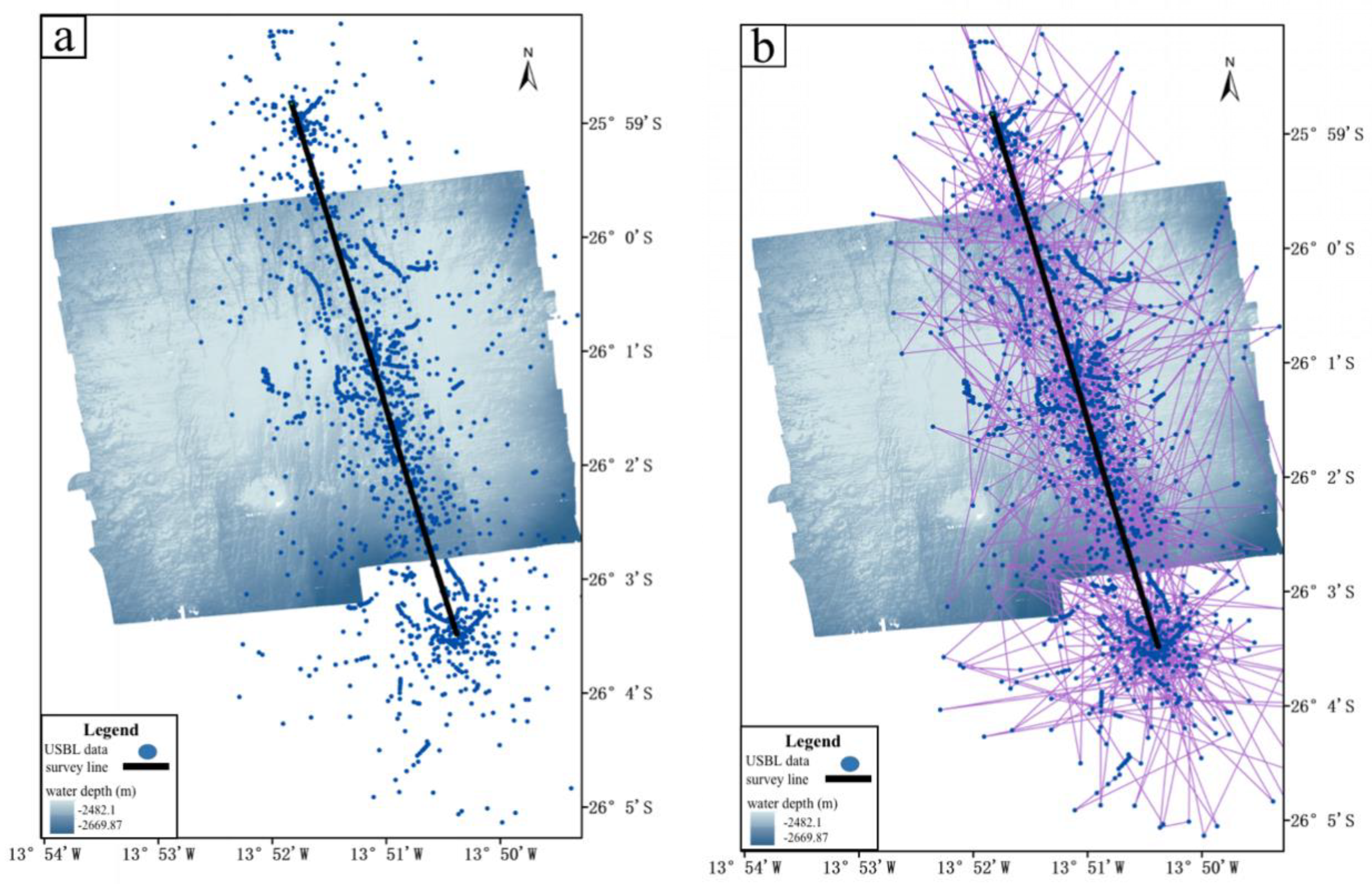
A USBL fixed to the platform is generally employed to achieve the underwater position fixing of the camera tow. However, not all lines were equipped with a USBL positioning system. Only 18 of the 28 lines surveyed in this area were equipped with an ultrashort baseline. Among them, 11 lines had UBSL data for the complete survey area and the remaining 7 had UBSL data for only part of the survey area. Among several survey lines acquired in the study area, some USBL positioning data were good. However, the USBL positioning data quality for some lines was poor, as shown in Figure 3a. The blue dots describe the camera’s USBL data, which can be very scattered along the way, and does not reflect the camera’s actual position. This situation is inevitable in seabed exploration and is not a minority.

In order to solve the camera data positioning problem, the depth data of the camera and the positioning data with better ultra-short baseline positioning signals were initially analyzed. The following conclusions were drawn.

By carefully analyzing the camera’s depth data, the depth data of the camera equipment is stable. During the detection operation, the up and down oscillation ranges are within 6 m. The maximum and minimum height from the seabed is 9 m and 1 m, respectively, basically stable at 5m, indicating a weak longitudinal oscillation of the camera. Therefore, the stability of the camera in operation is reliable.

We carefully analyzed the camera’s positioning data with better ultra-short baseline detection and positioning quality. An experiment with a sample of 5000 points indicates that the error range between the predicted positioning data and the original is within 5 m. It reflects that the lateral positioning error of the camera represented by the ultra-short baseline can be accurate within 5 m, that is to say, the camera’s lateral swing error is within 5 m.

According to the above analysis, the near-seabed camera towed body will not be disturbed too much during the operation of the seabed resource survey or it will not produce violent oscillation under no particular circumstances.

Figure 3a shows the shipboard GPS navigation positioning data during the near-bottom camera exploration operation. Figure 3b shows the USBL positioning data carried by the corresponding camera tow. A total of 2338 USBL positioning points were recorded for this survey line. When the USBL data were connected in chronological order, they could not correctly show the onboard underwater camera’s actual position and working path. The deviation of the displayed position information in the heading was also inaccurate compared to Figure 3a. The distance between the previous and the following positioning points varies up to 6 km in 1 s, which is impossible in practice.

Several analyses are performed to solve the position fixing camera data in this case. First, the ship will generally maintain a certain speed to work along the set survey line in the actual seabed resource survey operation. The ship will tow the camera tow for a near-seabed filming operation. Accordingly, the actual operation path of the camera tow is the same as the direction, path, and distance of the ship’s navigation in parallel, and the difference is negligible in a small area. Second, the camera tow is bound with a pressure sensor simultaneously, which can obtain high-precision distance data from the seabed and the sea surface and calculate the water depth profile of the camera survey line. It can be assumed that the water depth profile elevation data sequence recorded by the camera tow reflects the topographic profile information of the geographical location while the camera tow is working near the bottom. What is more, the area’s 1 m precision topographic data was obtained during the preliminary AUV survey operation, which can be employed as a background reference for the camera data. Since the area’s topography is highly variable and recognizable, it is easier to implement and validate the positioning correction using topographic alignment.

Therefore, subsequent attempts should be performed to match the water depth profile of the camera survey line with the profiles extracted from the high-precision topographic data of the study area acquired by the AUV. Accordingly, it is possible to find the most similar profile positions, verify the validity of the solution by combining data, such as shipboard and grab sampling records, and correct the positioning of the camera.

3. Methods

In order to match and correct the camera line, the following solution was adopted. First, the bathymetry data of the camera line was acquired, and the water depth profile of the camera survey line was generated. In order to facilitate the subsequent matching of similarity between the profile sequences and improve efficiency and accuracy, the profile segment sequence with greater undulation was selected as the camera line correction segment profile A (position is unknown, and the bathymetry value is the water depth data of the camera line). Second, the time record of profile A is checked, and the ship GPS data synchronized with the camera line (i.e., the position data of the ship’s route) is acquired to obtain the ship position “baseline” B, which is compatible with the time record of profile A. B’s starting and ending positions are obtained. Its length and direction angle are calculated to determine ship position B’s reference parameters. Then, according to the matching and correction requirements and the accuracy of AUV topographic data and topographic characteristics, the translation distance is adjusted to obtain topographic profiles with the same distance and direction as the ‘baseline’ B in large quantities from AUV high-precision topographic data. Accordingly, the profile set B {B₁, B₂, B₃, …, B_n} is formed. Finally, the DTW optimization algorithm matches the camera line correction section profile A with the topographic profile set B. The position of the profile with the highest similarity, B_i, is the geographic location of the camera tow in actual operation. Moreover, to realize the positioning correction of the camera tow, the position information of the sequence of Bi is read into the corresponding position sequence of the camera data. Figure 4 and Figure 5 show the schematic diagram of the textual method and the flow diagram of data acquisition and integration for fixing of camera data, respectively.

3.1. Extracting Profiles Big Data from Topographic Data

Python3.7 and an ArcGIS10.6 technical environment are employed to extract big data profiles from topographic data. The Technology Roadmap is shown in Figure 6. Within the object area’s high-precision water depth topographic data, many topographic profiles with the same direction and length as the object survey line (where the ship position profile B is located) are extracted as densely as possible according to the data accuracy and calibration accuracy requirements. These profiles are labeled in the order of extraction, and the data of each topographic profile is stored on the specified path to obtain a collection of profiles.

First, the baseline parameter is extracted, and the baseline is moved in parallel with a certain distance and direction so that the generated offset trajectory line set traverses the entire study area. The specific implementation method is as follows:

(1)

Import the acrpy, math, and pyproj modules required for data processing;

(2)

Employ the SearchCursor in the arcpy module to establish read-only access rights to return records from feature classes or tables, read the baseline parameters, and generate vector data;

(3)

Use the Transformer of the pyproj module to convert the baseline geographic coordinate value and the projected coordinate value to each other;

(4)

Use the Describe (lineFile) function of the arcpy module to obtain the baseline length in the x and y directions, and combine the floor function of the math module with the set translation parameters to ensure that the baseline is within the object area, east, west, north, and south orientations. Set the maximum number of offsets according to the batch translation direction;

(5)

Record the translated trajectory node coordinates in the array of the arcpy module, employ the Polyline function of the Arcpy module to convert the coordinate array into line elements, and utilize the InsertCursor function of Arcpy to write the line elements into the Shapefile;

(6)

Use Arcpy’s Merge function to label the vector data files composed of all the translated lines in the order of extraction and store the data of each offset track line on the specified path to obtain an offset trajectory line set.

Next, combine the high-precision water depth imaging data of the object area with the geographic location data of the offset trajectory lines after the above steps to extract and save the topographic profile data corresponding to each offset trajectory line in batches. Specific implementation steps are:

(1)

Use the Raster in the arcpy module to acquire the original raster data of the research area;

(2)

Use the Raster (Rasterfile) function of the arcpy module to obtain the grid range of the study area;

(3)

Use the StackProfile_3d function of the arcpy module to extract the topographic profile corresponding to each line in the line set according to the vector data file of the translation line set and the original raster data of the study area, saving the extracted profiles as a list;

(4)

In order to facilitate the calculation of the subsequent similarity, use the Table To Table conversion function of the arcpy module to convert the profile information list into a text file, and organize the data in the table to obtain the offline text file, which contains the elevation value sequence of the profile set.

3.2. Calculation of the Similarity between the Topographic Profile Sequence and the Water Depth Profile

The DTW algorithm [22] is a similarity measure that better matches the mapping of time series morphology by bending the time axis. Just such a technique, based on dynamic programming, has long been known to the speech-processing community [23,24,25]. Berndt and Clifford [26] employed the DTW algorithm to measure time series similarity. This algorithm can be utilized for similarity measures of time series of different lengths with good metric accuracy and robustness. It has been continuously improved [27,28,29] and is widely utilized in several fields [30,31,32,33]. The DTW algorithm measures the similarity between two sequences by bending, stretching, or shrinking the time axis. It can handle both equal-length and non-equal-length sequences. This algorithm overcomes the Euclidean distance problem for sequences that cannot be matched accurately after deformation. Lowe’s efficiency is superior to Euclidean distance and triangular similarity [34,35]. Euclidean distance data points can only be matched one-to-one. This algorithm compensates for this drawback and can simultaneously match data points of equal-length and non-equal-length sequences. Moreover, it supports appropriate stretching and bending operations on the time axis. The dynamic programming approach can be employed to find the optimal matching path with minimum bending cost while ensuring certain accuracy, thus forming offsets between time series data points and quickly matching to similar time series to achieve similarity metrics. The method is robust and can describe the specific shape of the time series. It can be employed for line shape comparison between near-bottom sounding bathymetric profiles and sea-level topographic profiles in the same region. In order to solve the localization problem of the sounding data, this paper applies this algorithm to the field of deep-sea solid resources for the first time.

In order to establish the DTW algorithm, two profile sequences A = (a₁, a₂, … a_i, …a_n) and B = (b₁, b₂, …b_j, … b_m) of length n and m are considered, where a₁ and b₁ denote the data points on the profile data sequence greater than or equal to a₁ and b₁, and less than or equal to a_n and b_m in the profile data sequence A and B, respectively. The adjacency distance matrix D_n×m = d (a_i, b_j) is constructed that the elements (i, j) in each matrix are aligned, corresponding to the points ai and b_j. A path is found from the top left corner to the bottom right corner such that the sum of the values of the elements through which the path passes is minimized to obtain the minimum value of the optimal matching path. Accordingly, the twisted curve is obtained. This means that the correspondence of the k points from the A sequence to the points in the B sequence is found. For example, if $\mathsf{\phi }\left(\mathrm{t}\right)$= (1,1), the first point in the A sequence corresponds to the first point in the B sequence. The principle of the DTW similarity measurement method is shown in Figure 7.

Further, the cumulative distance between the two time series can be obtained, as shown in Equation (1). Eventually, the most suitable twist curve minimizes the path’s cumulative distance, as shown in Equation (2).

$$D_{\phi }\left(A,B\right)={{\displaystyle \sum }}_{i=1}^{k}d\left({\phi }_A\left(t\right),{\phi }_B\left(t\right)\right)$$

(1)

$$\mathrm{DTW}\left(\mathrm{A},\mathrm{B}\right)=\min D_{\phi }\left(A,B\right)$$

(2)

The DTW distance allows sequence points to be self-replicated and then matched, supporting time axis bending and scaling. In the actual calculation process, the ‘quasi-symmetric step mode’ is utilized, and the loss matrix M is generated based on the distance matrix D and the step mode to a certain extent. It covers different constraints. $\mathrm{M}\left[\mathrm{i}\right]\left[\mathrm{j}\right]=\min (\mathrm{M}\left[\mathrm{i}-1\right]\left[\mathrm{j}\right],\mathrm{M}\left[\mathrm{i}\right]\left[\mathrm{j}-1\right],\mathrm{M}\left[\mathrm{i}-1\right]\left[\mathrm{j}-1\right]+\mathrm{D}\left[\mathrm{i}\right]\left[\mathrm{j}\right].$ Then, the value of the last column of the last row of the loss matrix is the minimum cumulative distance.

Based on the definition and the constraints, the DTW algorithm is established based on Equation (3).

$$\mathrm{M}\left[\mathrm{i}\right]\left[\mathrm{j}\right]=\left\{\begin{array}{cc}{(\mathrm{a}\left[0\right]-\mathrm{b}\left[0\right])}^2\hfill & \hfill \mathrm{i}=0,\mathrm{j}=0\\ {(\mathrm{a}\left[0\left]-\mathrm{b}\right[0\right])}^2+\mathrm{M}\left[0\right]\left[\mathrm{j}-1\right]\hfill & \hfill \mathrm{i}=0\\ {(\mathrm{a}\left[0\left]-\mathrm{b}\right[0\right])}^2+\mathrm{M}\left[\mathrm{i}-1\right]\left[0\right]\hfill & \hfill \mathrm{j}=0\\ {(\mathrm{a}\left[0\left]-\mathrm{b}\right[0\right])}^2+\mathrm{m}\mathrm{i}\mathrm{n}(\mathrm{M}\left[\mathrm{i}-1\left]\left[\mathrm{j}\right],\left[\mathrm{i}\right]\right[\mathrm{j}-1\right]\hfill & \hfill \\ \mathrm{M}\left[\mathrm{i}-1\right]\left[\mathrm{j}-1\right])\hfill & \hfill \mathrm{i},\mathrm{j}>0\end{array}\right.$$

(3)

Equation (3) indicates that $\mathrm{M}\left[\mathrm{len}\left(\mathrm{A}\right)-1\right]\left[\mathrm{len}\left(\mathrm{B}\right)-1\right]$ is the similarity distance $DTW\left(A,B\right)$ between sequences A and B. Then, the similarity distance can be transformed by $similarity=\frac{1}{1+DTW(A,B)}$ to obtain the similarity of sequences A and B.

3.3. Optimization of the DTW Algorithm

During the similarity calculation of topographic profile sequences with the DTW algorithm, it is found that some topographic profile data sequences have periodic fluctuation characteristics. At the same time, the monotonic advancement rates of their curves are inconsistent. During the calculation process of the above algorithm, it can be found that the path direction can only be adjusted to maintain the short-term monotonicity. This leads to the ‘ill-conditioned matching’ phenomenon in which the trends of the peaks and troughs are inconsistent while calculating the distance of the topographic profile sequence [37].

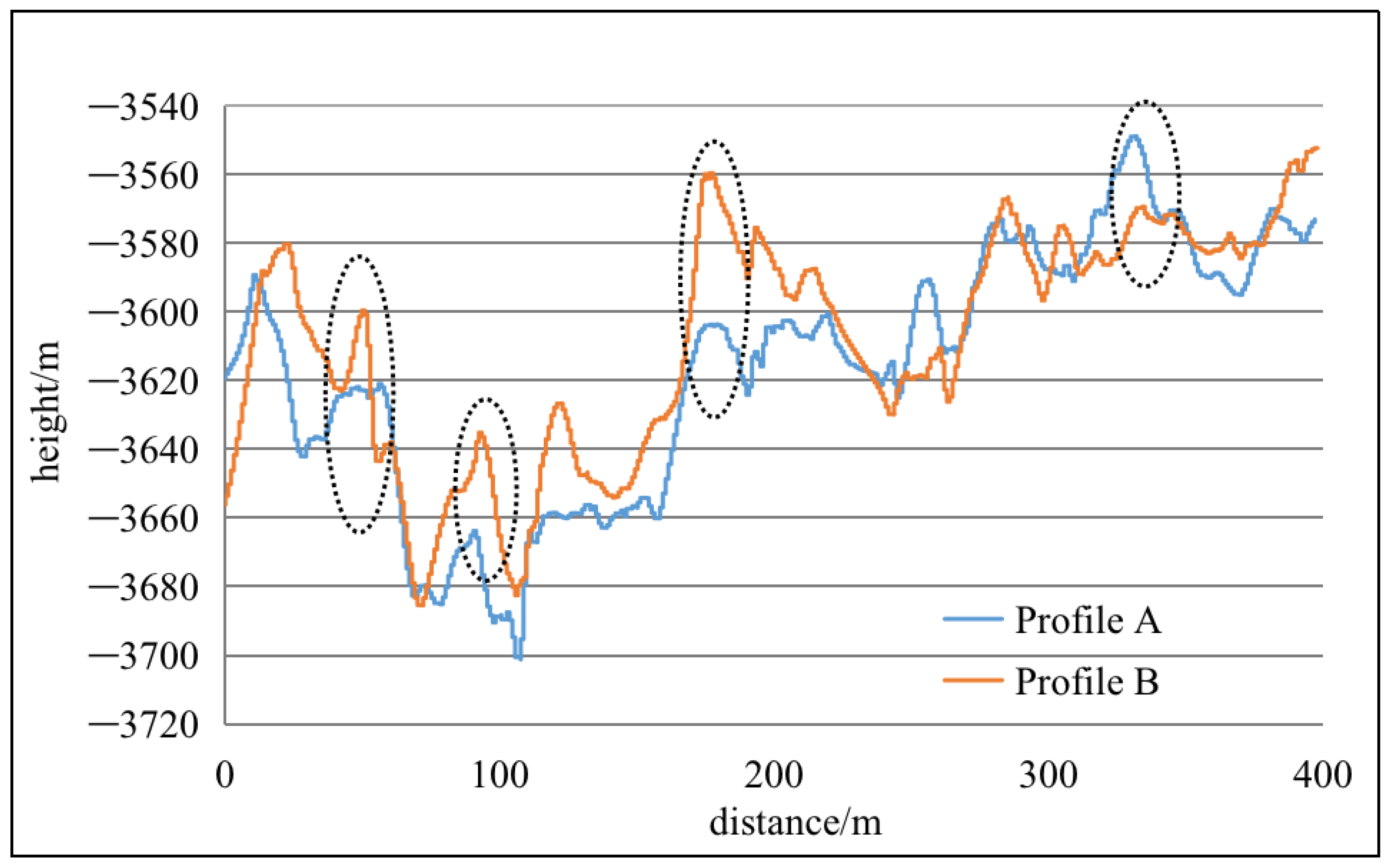
As shown in Figure 8, the distance between the two topographic profiles at the locations shown by the dashed circles is too significant, which increases the average distance between the two sequences, resulting in a ‘sick match’ during the matching process. The similarity of the regional trends can be satisfied by shifting the curves forward or backward, thus eliminating the effect of the ‘sick match’ on the similarity calculation. The longer the longest common substring of two series, the smaller the deviation and the magnitude of the required adjustment. Therefore, a penalty factor α is defined to adjust the original algorithm. The specific algorithm is as follows.

(1)

Calculate the maximum standard deviation sd_max. The mean values of the profile sequence A and B are denoted by $\overline{a}$ and $\overline{b}$, respectively; n and m denote the length of profile sequences A and B, respectively. Equations (4) and (5) describe the formulas for calculating the standard deviations of sequences A and B.

$$s{d}_A=\sqrt{\frac{{{\displaystyle \sum }}_{i=1}^n\left(a_i-\overline{a}\right)²}{n}}$$

(4)

Similarly, it follows that:

$$s{d}_B=\sqrt{\frac{{{\displaystyle \sum }}_{j=1}^m\left(b_j-\overline{b}\right)²}{m}}$$

(5)

Therefore, we have:

$$s{d}_{max}=\max \left(s{d}_A,s{d}_B\right)$$

(6)

(2)

Solve for the longest common substring and its length l. Since A and B are sequences of values in two profiles, the maximum standard deviation is set as the offset range, while solving for the longest common substring. The two values are within this standard deviation and are considered part of the common substring.

Let the length of sequences A and B be n and m, respectively. Define the matrix dp[i][j] (0 ≤ i < n, 0 ≤ j < m) according to Equation (7), where

$$\mathrm{dp}[\mathrm{i}][\mathrm{j}]=\left\{\begin{array}{ccc}0\hfill & \hfill \hfill & \hfill \mathrm{A}[\mathrm{i}]-\mathrm{B}[\mathrm{j}]\ge {\mathrm{sd}}_{\max }\\ 1\hfill & \hfill \mathrm{A}[\mathrm{i}]-\mathrm{B}[\mathrm{j}]<{\mathrm{sd}}_{\max }\hfill & \hfill \mathrm{i}\parallel \mathrm{j}=0\\ \mathrm{dp}[\mathrm{i}-1][\mathrm{j}-1]+1\hfill & \hfill \mathrm{A}[\mathrm{i}]-\mathrm{B}[\mathrm{j}]<{\mathrm{sd}}_{\max }\hfill & \hfill \mathrm{i},\mathrm{j}>0\end{array}\right.$$

(7)

The dynamic programming principle can be employed to find the optimal path of dp[i][j] from the top left corner to the bottom right corner. Accordingly, the longest common substring and its length l can be obtained.

(3)

Calculate the penalty factor using Equation (8).

$$\mathsf{\alpha }=1-\frac{{\mathrm{l}}^2}{\mathrm{n}\times \mathrm{m}}$$

(8)

$$similarit{y}_{update}=\frac{1}{1+\alpha DTW\left(A,B\right)}$$

(9)

In summary, this paper proposes an optimized DTW algorithm based on the principle of the longest common substring. This algorithm can eliminate the “sick match” phenomenon caused by the inconsistency of the peaks and troughs between two topographic profile sequences and facilitate the accurate calculation of the similarity between the two profile sequences.

4. Position Fixing of Camera Data

4.1. Data Preparation

The ship’s trajectory is an adjusted long-distance survey line in the actual survey of seabed resources. The video collected by the towed camera body during the ship’s journey is utilized to understand the seabed conditions and to discover seabed resources. The TV grab sampling can also determine whether to collect samples according to the video situation and simultaneously verify the camera data. Besides, the seabed topography varies, while some areas have apparent changes, and some are relatively gentle. According to the above characteristics, a specific survey line segment should be appropriately selected in the camera survey line as the calibration section of the camera line to achieve a better correction effect and to improve the calculation efficiency. This means that a segment of the mark is selected in the camera survey line to be corrected as the matching “baseline”. The “baseline” should be selected as the best section with hydrothermal sulfide (there are generally multiple ways to sample and provide validation), more pronounced topographic variations, and large topographic inflection points. The orange dashed and the solid lines in Figure 4 indicate the calibration section of the camera line and its corresponding ship position GPS data, respectively.

The GCS_WGS 1984 was employed to process the raw data of the object area (AUV high-precision topographic data of the study area) in ArcGIS to GRID raster format with data ranges −13.85800~−13.845994 and −26.037005~−25.999996 and data accuracy of 1 m × 1 m. The selected ‘baseline’ data range is −26.016742~−26.019834 and −13.852539~−13.851571 with a Shapefile spatial data type, using the GCS_WGS_1984 spatial reference coordinate system, whose datum is D_WGS_1984.

4.2. Method Application

A Python script was written based on the above method to batch the calibration section of the camera survey line in the study object area at 10 m intervals from east to west and north to south. Accordingly, all the trajectory lines generated after the offset were parallel to the object survey lines traversing the raster layers of the object area. Due to many offset trajectory lines, a Shapefile was generated for every 10,000 offset trajectory lines and saved for processing in batches, considering the efficiency of the single machine calculation.

Figure 9, shows that 47,627 offset trajectory lines parallel to the object survey line were obtained after offsetting. The file was named offLines_merge, a Shapefile spatial data type, geographic coordinate system GCS_WGS_1984, and datum D_WGS_1984.

The corresponding elevation data sequences of 47,627 topographic profiles are extracted in batches from the AUV high-precision topographic data of the object area according to the geographic location data of the above offset trajectory lines.

Table 1. Sequential list of elevation data for selected topographic profiles (partial).

Euclidean Distance from the Start of the Profile/m	Elevation Value of the Profile Sequence/m
	Profile_1	Profile_2	Profile_3	……	Profile_47626	Profile_47627
0	−2593.4	−2637.1	−2638.5	……	−2604.5	−2605.3
1.1	−2593.8	−2637.1	−2638.6	……	−2604.4	−2605.2
2.2	−2593	−2638.1	−2638.5	……	−2604.6	−2605.1
3.2	−2591.9	−2637	−2638.7	……	−2604.6	−2605
4.3	−2591.8	−2637.1	−2638.8	……	−2604.3	−2604.8
5.4	−2591.3	−2637.2	−2638.9	……	−2604.4	−2604.7
6.5	−2591.5	−2637.3	−2639.1	……	−2604.3	−2604.5
7.6	−2591.5	−2637.4	−2639.3	……	−2604.1	−2604.9
8.6	−2592.7	−2637.6	−2639.6	……	−2603.9	−2604.5
9.1	−2594.9	−2638	−2639.9	……	−2603.7	−2604.6
9.7	−2592.7	−2638.4	−2640.2	……	−2603.5	−2604.7
10.8	−2592.9	−2638.8	−2640.4	……	−2603.4	−2604.8
11.9	−2591.9	−2639.1	−2640.6	……	−2603.3	−2604.9
13	−2592.7	−2639.3	−2640.7	……	−2603.3	−2604.9
14	−2596.7	−2639.4	−2640.7	……	−2603.3	−2604.7
15.1	−2597	−2639.5	−2640.8	……	−2603.3	−2604.6
……	……	……	……	……	……	……
338.2	−2623	−2651.6	−2650.4	……	−2583.9	−2585.2
339.3	−2623.7	−2651.8	−2650.5	……	−2583.7	−2585.1
340.4	−2623.7	−2651.9	−2650.6	……	−2583.5	−2585
341.5	−2623.8	−2652	−2650.8	……	−2583.3	−2584.7
342.5	−2623.9	−2652.1	−2651	……	−2583.1	−2584.3
343.6	−2623.7	−2652.1	−2651.1	……	−2582.9	−2583.9
344.7	−2623.6	−2652.2	−2651.3	……	−2582.8	−2583.5
345.8	−2624	−2652.3	−2651.5	……	−2582.7	−2583.1

presents the elevation data sequences of some topographic profiles, the full data is available in the Supplementary Materials.

In order to calculate the similarity between 47,627 topographic profile elevation data sequences and the camera’s water depth profile sequence of the camera survey line correction section, the DTW optimization algorithm is constructed based on Python language, and the similarity calculation results are stored in a text file. The specific implementation steps include: (1) import the NumPy, math, and panda modules required for data processing; (2) take the water depth data sequence of the matching calibration section profile A as the matching object, and calculate the similarity with the profile set B {B₁, B₂, B₃, ……, B_n} profile elevation data sequences; (3) calculate the maximum standard deviations between profile A and the sequences in profile set B; (4) calculate the longest common substring and its length between profile A and the sequences in profile set B; (5) calculate the optimization penalty coefficient α between profile A and the sequences in profile set B; (6) combine the penalty coefficient α and calculate the minimum distance and the optimized similarity between camera profile A and the sequences in profile set B; (7) repeat steps (2) to (6); and (8) rank the calculated optimized similarity and output the result.

4.3. Camera Data Position Fixing

Table 2. Similarity matching results for 10 m interval topographic profiles sequence(partial).

Serial Number of the Profile	$Similarit{y}_{update}$
profile_4331	91.30%
profile_4332	85.00%
profile_4333	83.30%
profile_4330	82.50%
profile_5147	82.40%
profile_23966	82.00%
profile_36114	81.90%
profile_40218	81.60%
profile_4795	80.90%
profile_10625	80.20%
profile_376	79.20%
profile_29874	73.40%
profile_33647	73.40%
profile_5603	72.60%
profile_19852	71.30%
profile_41597	67.10%
profile_11963	66.90%
profile_26149	66.40%
profile_33065	65.80%
profile_2063	64.40%
……	……

shows the partial similarity matching results for sequences of profiles spaced ten meters apart, the full data is available in the Supplementary Materials. It was found that the profile elevation data sequence of profile_4331 has the highest similarity to the water depth data sequence of the object survey line (91.3%).

In order to determine the location of the camera survey line, a range of 550 m north-south and 300 m east-west is taken as the center of the location of the profile_4331, a profile matched by the above method operation. Within this range, the object line’s raster data is offset in batches at 1 m intervals from east to west and north to south. All the offset trajectory lines parallel to the object line are generated after traversing the offset within the raster layers of the object area. After offsetting, 49,842 offset trajectory lines parallel to the object survey line are obtained. The geographic location data of the offset trajectory lines are then combined with the high-precision water depth data of the object area in the above step. Then, the 49,842 topographic profiles corresponding to the offset trajectory lines are extracted. The DTW optimization algorithm is employed to calculate the sequence of 49,842 topographic profiles in batch and the water depth profile data sequence.

Table 3. Similarity matching results for 1-m interval topographic profiles sequence (partial).

Serial Number of the Profile	$Similarit{y}_{update}$
profile_4331_26851	95.90%
profile_4331_28652	93.10%
profile_4331_26850	92.70%
profile_4331_26853	91.30%
profile_4331_39723	88.60%
profile_4331_891	87.90%
profile_4331_29047	86.30%
profile_4331_47829	86.00%
profile_4331_5182	85.70%
profile_4331_83	85.50%
profile_4331_39021	85.30%
profile_4331_11548	84.60%
profile_4331_17406	84.40%
profile_4331_28749	82.60%
profile_4331_27910	82.30%
profile_4331_33905	82.10%
profile_4331_14803	81.90%
profile_4331_9201	81.40%
profile_4331_8493	80.80%
profile_4331_44920	80.40%
……	……

, shows that the partial similarity between the profile elevation data sequence of profile_4331_26581 and the water depth data sequence of the object survey line is the highest, 95.9%. What’s more, the full data is available in the Supplementary Materials. It can then be judged that the geographical location of profile_4331_26581 is the actual location of the camera survey line.

Based on profile_4331_26581, the entire camera survey line is matched to this position using the camera survey line calibration section profile. The position information of profile_4331_26581 is acquired from the profile sequence to the position sequence corresponding to the camera data using the above method. The camera data positioning is corrected to extract the position corresponding to the entire camera survey line in the AUV topographic data. This allows the camera data to be positioned within the topographic accuracy of the submarine camera data, as shown in Figure 10.

5. Discussion

At present, the positioning of near-bottom camera data, as the most intuitive and effective means of detecting hydrothermal sulfide on the seafloor, is the most critical issue to avoid compromising the use and value of the camera data. In the South Atlantic mid-ridge seafloor hydrothermal surveys, equipment position fixing is achieved using a USBL positioning system (USBL) attached to the camera tow. High-quality USBL data can be utilized to locate underwater survey equipment and its detection data by correcting the USBL positioning data to solve the position fixing problem [38,39,40,41,42,43,44]. These methods are suitable for positioning data with low dispersion of anomalies, relatively few error points, and good overall quality. If the USBL data signal is extremely poor or even missing, the above methods cannot be helpful.

Thus, by correcting the USBL positioning data to locate the underwater survey equipment and its detection data, the positioning data with fewer discrete outliers, fewer error points, and better comprehensive quality can be obtained. The above method cannot accurately locate and correct the precious data collected by the submarine detection equipment under extremely poor or missing USBL data signal due to signal interference and environmental state changes.

As explained by the above analysis (2.2), the near-seabed camera towed body will not be disturbed too much during the operation of the seabed resource survey or it will not generate violent oscillation under no particular circumstances. Besides, topographic variations cannot lead to abrupt changes in morphological characteristics. Therefore, the DTW algorithm can perform subsequent similarity matching. Based on Python language and an ArcGIS technology environment, this paper constructs the background information of the camera survey line and AUV high-precision topographic data. The typical matching calibration section profile is selected in the camera survey line to be calibrated. It is employed as the profile shape reference, with the parameters of position, direction, and distance extracted based on the GPS position fixing information on board the ship simultaneously. The topographic profile in the AUV topographic is extracted according to specific density rules, and the optimized DTW algorithm is utilized to traverse all the topographic profiles and calculate the similarity between the bathymetric profile of the camera survey line calibration section and the topographic profile. Accordingly, the profile with the highest matching degree is the correct position of the camera survey line calibration section. Moreover, the camera survey line’s position matching and positioning correction are performed, thus realizing the positioning correction of the camera data. In addition, the position fixing problem of the survey data has been solved using an optimized DTW algorithm, leaving aside the USBL positioning data in the near-bottom survey. Furthermore, the underwater position fixing problem that cannot be solved by GPS and USBL positioning systems is solved.

Besides, while calculating the similarity of topographic profile sequences using the DTW algorithm, the monotonicity of their curves advances at inconsistent rates due to the periodic undulating characteristics of specific topographic profile sequences. The “sick match” phenomenon with inconsistent peak and trough trends appears, as shown in Figure 8. This paper improves and optimizes the original algorithm. A penalty coefficient α is defined to eliminate the “sick match” phenomenon and facilitate an accurate calculation of the similarity between two profile sequences.

The effectiveness of the presented solution can be validated in two ways.

Firstly, it can be seen from the above calculation (4.1, 4.2) that the matching results of two degrees of precision are unique. The matched profile similarity of the profile extracted with a 10 m data interval is 91.3%. Based on the matching result, the precise matching of the 1 m data interval is performed, and the similarity is improved to 95.9%, indicating that the actual matching result is within the range indicated by the target. The remaining 4% of the similarity difference may be due to other uncertainties. Moreover, the comparison through station sampling is also compatible with the actual situation. Therefore, the proposed method is feasible and can solve the camera data locating problem under uncertain ultra-short baseline location data. Secondly, the method’s validity can be further verified based on data, such as shipboard and grab sampling records. Data calculations show that the calibration section of the camera tow is approximately 1523 m away from the mother ship’s GPS position in the north-south direction and 109m away in the east-west direction, with the mother ship being 99.8 m long and 17.8 m wide. Since the GPS positioning device of the mother ship is located at the bow and the cable hanging the optical camera tow is located at the stern, the actual calibration position of the camera tow and the position of the cable hanging from the mother ship should be approximately 1423 m and 109 m apart in the north-south and east-west directions, respectively. The projection distance between the camera tow and the ship’s suspension cable position is approximately 1427.2 m.

According to the towing operation records of the voyage, when the ship traveled to the section selected for the experiment, it maintained a uniform speed of 1.0 Kn. The average cable length of the camera tow was approximately 2921 m, and the average depth of the optical camera tow was approximately 2610 m.

Based on the average depth of the optical camera tow during operation (approximately 2610 m) and the projected distance between the calibration position of the camera tow and the position of the ship’s suspended cable (approximately 1427.2 m) calculated in the previous section, the spatial distance between the position of the ship’s suspended cable and the calibration position of the camera tow is obtained as approximately 2974.7 m. Accordingly, after the positioning calibration of the camera tow by the proposed method, the length of the cable towed by the ship during operation is approximately 2974.7 m. This calculation results in a cable length that differs by approximately 53.7 m from the cable length recorded in the operational shift report for the voyage. The resultant positioning fixing position is credible, considering the effects of wind and waves, systematic errors, manual measurements, and other factors. It also further demonstrates the feasibility and effectiveness of the proposed method.

In terms of the efficiency of the proposed method, it took approximately 16 h to compute and initially match tens of thousands of profiles extracted at 10 m intervals over a 7 km area using a dual-core general office computer. Moreover, it took approximately 18 h to match nearly 50,000 profiles in further precision matching. Based on this efficiency estimate, processing with a high-performance server can be performed in less than an hour, a task that cannot be performed manually. Validation has indicated that the algorithm is fast, effective, and accurate, with the correction accuracy being the topographic accuracy. It can effectively solve the problem of not being able to perform accurate positioning based on USBL positioning data when it is highly abnormal. It also solves the problem of underwater position fixing that GPS and other global positioning systems cannot resolve.

6. Conclusions

This paper addresses the problem of complex positioning data in near-seabed sounding, especially for the confusing USBL positioning data, and corrects the visual data positioning using extensive data of near-seabed high-precision topographic profiles. Accordingly, it can solve the seabed position fixing problem that cannot be solved by GPS, USBL, and other positioning methods.

The DTW algorithm is first introduced into a seabed data location application. It is optimized with penalty coefficients to calculate the similarity between the camera line correction section profile and the topographic profile. The method is implemented based on Python language and an ArcGIS technical environment. The maximum similarity in the experiments is 95.9% and the topographic accuracy determines the correction error size, which is compatible with topographic accuracy. The verification and test results demonstrate that the algorithm is fast, effective, and accurate and can solve the position fixing problem of towed exploration equipment and its acquired data. The proposed algorithm is expected to be promoted, while fixing subsequent seabed survey equipment.

The conditions or limitations of this solution are the requirements for the near-bottom survey equipment to simultaneously acquire bathymetric data during the survey operation and the requirement to accomplish high-precision topographic surveys of the same area (performed for an unlimited period).