Potential of Phase-Amplitude-Based Multi-Scale Full Waveform Inversion with Total-Variation Regularization for Seismic Imaging of Deep-Seated Ores

Abstract

As the demand for ore resources increases, the target for mineral exploration gradually shifts from shallow to deep parts of the Earth (>1 km). However, for the ore-hosting strata, it is difficult to obtain high-resolution images by using the electromagnetic method. Seismic full waveform inversion (FWI) is an optimization algorithm which aims at minimizing the prestack seismic data residual between synthetic and observed data. In this case, FWI provides an effective way to achieve high-resolution imaging of subsurface structures. However, acquired seismic data usually lack low frequencies, resulting in severe cycle skipping of FWI, when the initial velocity model is far away from the true one. Phase information in the seismic data provides the kinematic characteristics of waves and has a quasi-linearly relationship with subsurface structures. In this article, we propose to use a phase-amplitude-based full waveform inversion with total-variation regularization (TV-PAFWI) to invert the deep-seated ores. The ore-hosting velocity model test results demonstrate that the TV-PAFWI is suitable for high-resolution velocity model building, especially for deep-seated ores.

1. Introduction

The seismic reflection method has great potential for deep structure imaging, which meets the requirements of mineral exploration for deep-seated ore deposits (>1 km) [1,2,3,4,5,6,7,8]. A high-quality velocity model is needed to obtain a high-resolution reverse time migration (RTM) image of deep-seated ores. However, the structures of ore bodies are usually irregular, and produce a mass of scattering waves, which result in poor resolution of seismic inversion and imaging results. Seismic full waveform inversion (FWI) is an optimization algorithm which aims at minimizing the prestack seismic data residual between synthetic and observed data [9,10,11,12,13]. In this way, FWI provides an effective way to achieve accurate velocity inversion and has great potential for subsurface structures imaging.

In recent years, the FWI-based new methods have already been successfully applied in mineral exploration and obtained effective results. Sun et al. proposed a new energy compensation strategy for elastic FWI to retrieve the deep-seated ores [14]. Mao et al. used an adjoint-state method to invert the source function and used a data similarity-based misfit to build velocity model used for imaging the ore-hosting strata [15]. Xing et al. proposed an energy spectrum-based FWI misfit to build a better ore-hosting velocity model [16]. Singh et al. used 3D FWI method to build a velocity model for an iron-oxide mining model [17]. Zhang et al. used the multisource FWI method to invert the ore bodies [18]. However, low-frequency seismic data below 6 Hz is still extremely important to retrieve low-wave-number structures and avoid cycle skipping of FWI [19,20,21,22,23,24,25,26,27].

In seismic exploration, it has been proven that phase components are similar to the travel time and have a quasi-linearly relationship with the subsurface structures [28,29,30,31,32,33,34]. In this way, the phase information has great potential to design a more linear misfit for initial velocity model building. In recent years, seismic data phase information-based FWI misfit has developed rapidly [28,29,30,31,35]. In addition, correlation-based FWI misfit functions focus on the phase similarity and relax the requirement for amplitude matching between synthetic and observed data [36,37,38,39,40]. Furthermore, adaptive matching filter-based FWI misfit functions are also a kind of phase adjustment approach, which can effectively invert subsurface structures [41,42,43,44].

In this article, to improve the inversion results of ore bodies, we introduce a phase-amplitude-based full waveform inversion (PAFWI) misfit function to focus on the phase similarity. In the PAFWI misfit function, the amplitude weights are reduced by an amplitude factor, making it possible to emphasize measuring the phase similarity between synthetic and observed data. First, we will review the traditional FWI method, and we show a phase-amplitude-based full waveform inversion with total-variation regularization (TV-PAFWI) method and derive its corresponding gradient. After that, we compare TV-PAFWI with different parameters to prove that the new method is an effective approach to invert the deep-seated ores. Finally, we test the TV-PAFWI stability in handling strong Gaussian noise.

2. Review of Full Waveform Inversion

For a 2D constant density acoustic FWI, the wave equation can be defined as:

$$\frac{{\partial }^{2}u}{\partial x^2}+\frac{{\partial }^{2}u}{\partial z^2}-\frac{1}{v^2}\frac{{\partial }^{2}u}{\partial t^2}=f(t)\delta (x-x_s),$$

(1)

where $u$ is seismic wavefield, $f(t)$ is source signature, $x_s$ is the source position, and $v$ denotes P-wave velocity model. In this case, we can formulate a least-square-based FWI misfit function, which measures the discrepancy between the synthetic and observed data as follows [10,11,12]:

$$J\left(v\right)=\frac{1}{2}{\displaystyle \sum _s{\displaystyle \sum _r{\displaystyle \underset{}{\int }{\Vert u-d\Vert }_2^2}}}\begin{array}{c}\begin{array}{c}dt\end{array}\end{array},$$

(2)

where $d,u$ in the FWI misfit function indicates the observed and synthetic data, respectively; $s$, $r$ indicates the number of shots and receivers, respectively. The chain rule—based partial derivative of the objective function is,

$$\frac{\partial J\left(v\right)}{\partial v}={\displaystyle \sum _s{\displaystyle \sum _r{\displaystyle \underset{}{\int }\left(u-d\right)}}}\frac{\partial u}{\partial v}\begin{array}{c}\begin{array}{c}dt\end{array}\end{array},$$

(3)

Therefore, according to the adjoint-state method [11], the adjoint source of FWI is denoted as

$$f_s^{}=\left(u-d\right),$$

(4)

Therefore, the FWI gradient is denoted as,

$$\frac{\partial J\left(v\right)}{\partial v}=-\frac{2}{v^3}{\displaystyle \sum _s{\displaystyle \underset{}{\int }\frac{{\partial }^2{P}_f^{}}{\partial t^2}{P}_b^{}}}\begin{array}{c}dt\end{array},$$

(5)

where the $P_f$ and $P_b$ are the forward and back-ward wavefields. We update the velocity parameter $v$ using the steepest descent method, and it can be written as:

$$v_{k+1}=v_k-{\alpha }_k{g}_k,$$

(6)

where $g_k=\partial J\left(v\right)/\partial v$ denotes the gradient direction of TV-PAFWI misfit function. ${\alpha }_k$ is the step length for kth iteration.

3. PAFWI with Total-Variation Regularization

When the seismic data lack low frequencies, it poses a great challenge for the traditional FWI to invert the deep-seated ore bodies [19,20,21,22,23,24,25,26,27]. This is because the reflection wave-based FWI misfit function shows strong nonlinear characteristics and leads to cycle skipping in the FWI process [10,11,28,32,38]. In this case, the least-squares-based PAFWI method is proposed, which helps to boost the deep reflections, and reduce amplitude constraints. In addition, to suppress imaging artifacts, we incorporated the total-variation regularization method with the PAFWI misfit function as follows,

$$J\left(v\right)=\frac{1}{2}{{\displaystyle \sum _s{\displaystyle \sum _r{\displaystyle \underset{t}{\int }{\displaystyle \underset{\omega }{\int }\left|\begin{array}{c}\end{array}{\left|\tilde{u}\right|}^p{e}^{i{\phi }_u}-{\left|\tilde{d}\right|}^p{e}^{i{\phi }_d}\begin{array}{c}\end{array}\right|}}}}}^2\begin{array}{c}dtd\omega \end{array}+\eta {\lambda }_{TV}{\Vert v\Vert }_{TV},$$

(7)

where $J\left(v\right)=J_{data}\left(v\right)+J_{TV}\left(v\right)$; $\tilde{u}$, $\tilde{d}$ are the synthetic and observed data in the time–frequency domain. The amplitude factor $p\in \left[0,1\right]$ is used to redistribute the phase and amplitude proportions. ${\lambda }_{TV}$ is used to adjust the weights of data and model constraints. However, in TV-PAFWI misfit function, we first need to normalize the value of data misfit and the model constraints. Therefore, another weighting factor $\eta =\max \left(\left|g_{data}\right|\right)/\max \left(\left|g_{TV}\right|\right)$ is introduced, where $g_{data}$ is the gradient of $J_{data}\left(v\right)$ and $g_{TV}$ is the gradient of $J_{TV}\left(v\right)$.

The chain rule—based partial derivative of TV-PAFWI misfit function is

$$\begin{array}{r}\frac{\partial J\left(v\right)}{\partial v}={\displaystyle \sum _s{\displaystyle \underset{t}{\int }{\displaystyle \underset{\omega }{\int }\mathrm{Re}\left\{\left(\Delta D\right){\left[p\left({\left|\tilde{u}\right|}^{p-1}\right)\left(e^{i{\phi }_u}\right)\frac{\partial \left|\tilde{u}\right|}{\partial v}+{\left|\tilde{u}\right|}^p\frac{\partial }{\partial v}\left(e^{i{\phi }_u}\right)\right]}^{*}\right\}}}}dtd\omega +\\ \frac{\partial }{\partial v}\left({\displaystyle {\int }_{\Omega }\sqrt{\beta +v_x^2+v_z^2}}dxdz\right)\end{array}$$

(8)

where $\Delta D={\left|\tilde{u}\right|}^p{e}^{i{\phi }_u}-{\left|\tilde{d}\right|}^p{e}^{i{\phi }_d}$, and $\beta$ is a small positive number to avoid dividing over zero. The gradient of TV-PAFWI misfit function is as follows,

$$\begin{array}{r}\frac{\partial J\left(v\right)}{\partial v}={\displaystyle \sum _s{\displaystyle \underset{t}{\int }\mathrm{Re}{\left\{W_h{}^{-1}\left\{\frac{\mathrm{Re}\left[\left(p-1\right)\left(\Delta D\right){\left(\tilde{u}\right)}^{*}\right]\begin{array}{c}\tilde{p}\end{array}+\left(\Delta D\right){\left|\tilde{u}\right|}^2}{{\left|\tilde{u}\right|}^{3-p}}\right\}\right\}}^{{}^{}}\frac{\partial u}{\partial v}}}dt-\\ \eta {\lambda }_{TV}\left[\frac{v_{xx}^{}\left(v_z^2\right)+v_{zz}^{}\left(v_x^2\right)-2v_x^{}{v}_z^{}{v}_{xz}^{}+\beta \left(v_{xx}^{}+v_{zz}^{}\right)}{{\left(\beta +v_x^2+v_z^2\right)}^{\frac{3}{2}}}\right]\end{array}$$

(9)

where $W_h^{-1}[\cdot ]$ means inverse Gabor transform. For more details, please refer to Appendix A, Appendix B and Appendix C. Therefore, according to the adjoint-state method, the TV-PAFWI gradient can also be obtained by the wave-field correlation.

4. Numerical Test

A complex ore-hosting velocity model (Figure 1) is modified from a geological model in the Luzong Basin, China. In the middle of model, it consists of multiple ore bodies, which is the target region of our FWI method testing. From Figure 1, it shows that the ore bodies present gently lenticular with dome-like geometry. In the the target region, there are only 3 large ore bodies, and the rest are small ore bodies. In addition, the center is dominated by leached poor iron ore, with rich and thick ore surrounding it [14,45]. However, with the poor quality seismic data and complexity of geological structures in ore areas, it poses a great challenge for the traditional FWI to invert the ore bodies, especially in the deep regions.

In this numerical test, the size of the ore-hosting velocity model is $7.0 \times 2.5 \mathrm{km}$ (Figure 2). There are 20 shots and 280 receivers distributed on the top of the ore-hosting velocity model. The recording time is 3.2 s, with a 2 ms time interval. To better match the filed datasets, in this case, a low-cut 6 Hz Ricker wavelet with a dominant frequency of 15 Hz is used to test the ability of low-frequency dependence (Figure 3). In addition, we consider the frequency-based multiscale strategy, and define the frequency band of 6–12 Hz as low-frequency data, and the frequency band of 6–20 Hz is as high-frequency data. In this section of numerical test, first, we give a detailed analysis of the adjoint sources. Then, a comparison of results TV-FWI and TV-PAFWI is shown in the numerical tests. In addition, we also show the different TV parameter and amplitude factor test results. Finally, a commonly used Gaussian noise was applied to test the anti-noise ability of the PAFWI and TV-PAFWI methods.

4.1. The PAFWI Adjoint Sources

To explain the characteristic of the time–frequency phase and amplitude information, in Figure 4, we show the adjoint sources with different amplitude factors in the time–space domain. In Figure 4a, we see the PAFWI adjoint source with amplitude factor p = 1, which is similar to the adjoint source of traditional FWI. The amplitude factor in the PAFWI misfit function was then gradually decreased to reduce the amplitude constraints. Comparisons in Figure 4a–c demonstrate that the PAFWI adjoint sources with p = 0.6 and p = 0.3 show clear reflection signals, especially for the deep parts. However, when the PAFWI amplitude factor is set to p = 0, it is a pure phase misfit function which contains too much phase artifacts, leading to an unstable inversion algorithm. Therefore, the amplitude information is also significant for the seismic waveform inversion. In this case, to fully use the linear characteristics of the phase information while avoiding the problems of algorithm instability and gradient imbalance, the PAFWI amplitude factor should be set between 0.3 and 0.6.

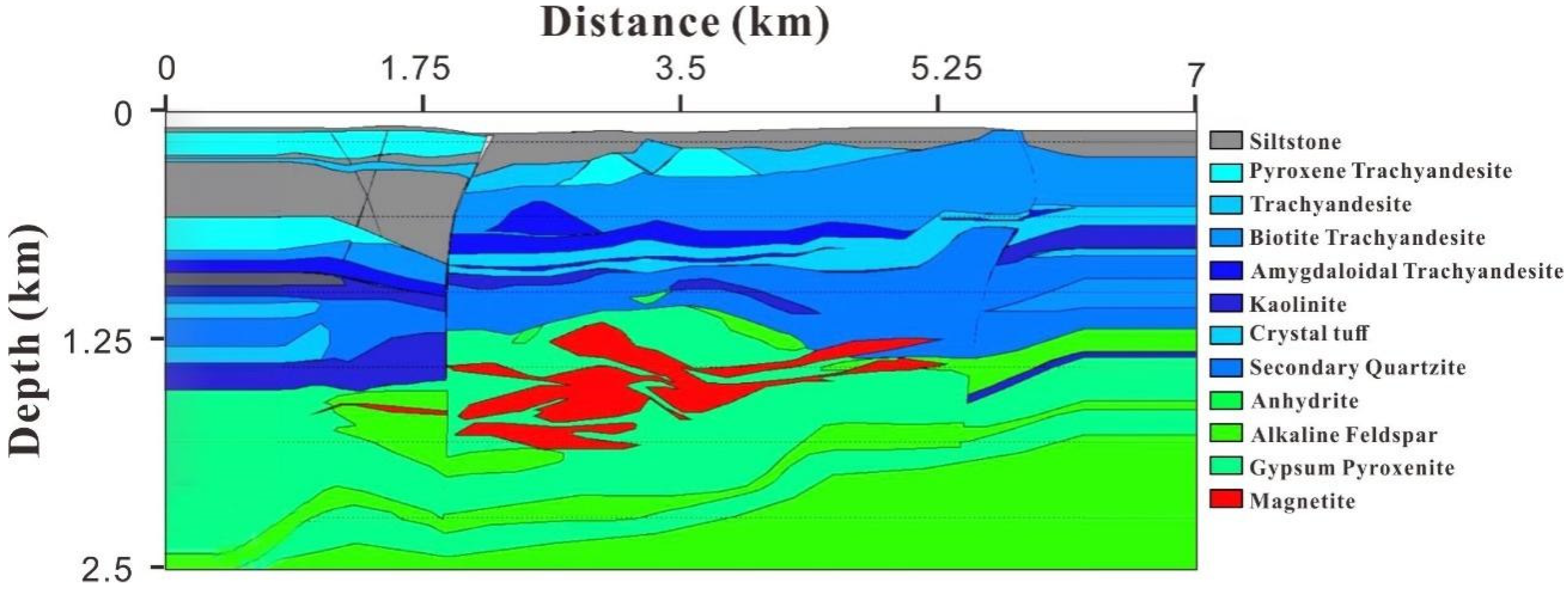
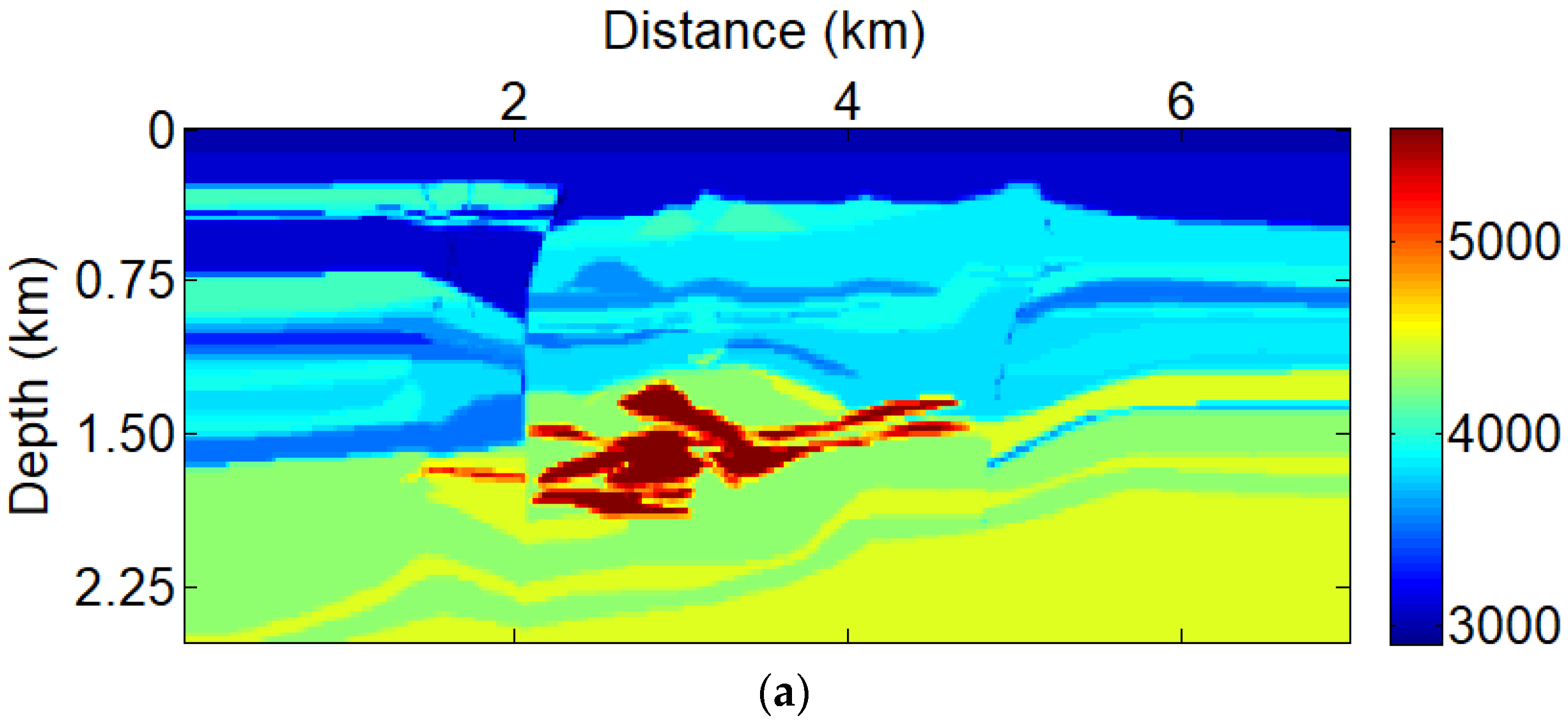
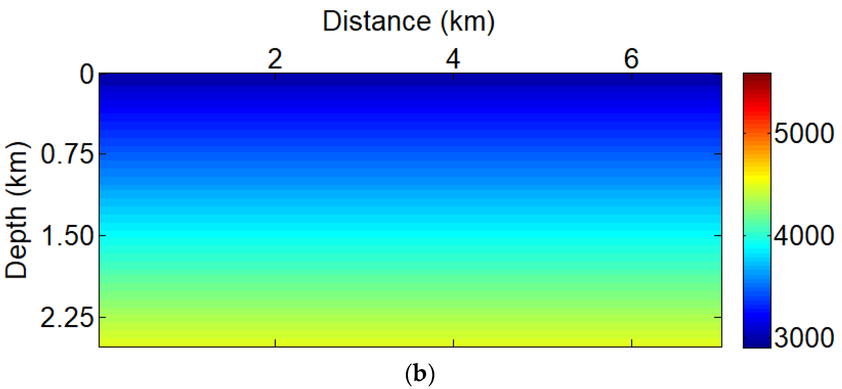
4.2. Ore-Hosting Model Test

Now, the numerical tests of low frequency seismic data-based TV-PAFWI results with different amplitude factors are shown in Figure 5. Comparisons in Figure 5a–d demonstrate that the TV-PAFWI with p = 0 shows strong phase artifacts. A comparison of Figure 5d with Figure 5b,c shows that the ore bodies inverted by the TV-PAFWI method seem better than the TV-FWI result. This is due to a purely exponential phase misfit function, resulting in the almost equal weighting of weakly scattered and strongly scattered seismic signals from direct wave to reflection wave. In addition, the subsurface structure is too complex to fully understand the propagation of seismic waves, and even the smallest perturbation of the wave field can cause strong changes in the phase characteristics of the seismic data. In addition, if the exponential phase information without amplitude weight is used for seismic inversion, the PAFWI process may be unstable, and even the problem of gradient imbalance may be encountered. The inversion result shows that the amplitude information is significant for the TV-PAFWI misfit function.

Then, the TV-PAFWI results with low-frequency seismic data are regarded as an initial velocity model to improve the resolution of the ore bodies, as shown in Figure 6. Comparison of Figure 6a–d shows that the TV-PAFWI with p = 0.3–0.6 can better recover the ore bodies. In comparison of Figure 6a with Figure 6b, we see that the quality and resolution of the ore bodies have been greatly improved, and the deep structures can be seen clearly. The velocity profiles with different methods are shown in Figure 7. The velocity comparisons show that the TV-PAFWI with p = 0.3–0.6 can obtain inversion results. Therefore, in this case, the amplitude factor was chosen as p = 0.3–0.6 for the ore-hosting velocity model inversion.

To further compare the inverted velocity values, we show some depth profiles at 3.5 km for TV-PAFWI results with different amplitude factors. From the comparison results in Figure 6a–d, it can be seen that the TV-PAFWI results with amplitude factors between 0.3 and 0.6 are more similar to the true velocity parameters. In contrast, the other results are inconsistent with the profiles of the true velocity parameters. As can be seen from the test results in Figure 7, the phase component can improve the inversion results, but the amplitude information also needs to be preserved in the TV-PAFWI misfit function.

4.3. TV Parameter Test

In the TV-PAFWI misfit, the coefficient ${\lambda }_{TV}$ balances the confidence level between the data misfit function and the regularization term. Therefore, an appropriate regularization coefficient (${\lambda }_{TV}$) is important to constrain the model inversion. In this case, a simple TV parameter selection procedure is applied to test the PAFWI methods. For example, in Figure 8, we set ${\lambda }_{TV}=0$ and ${\lambda }_{TV}=1$, respectively. Figure 8a shows that the TV-PAFWI is strongly affected by the phase artifacts, when amplitude factor p = 0 and ${\lambda }_{TV}=0$. This is because the PAFWI misfit function has great potential for enhancing deep reflections and introducing imaging artifacts. The comparison results of Figure 7b and Figure 8a show that the TV-PAFWI with amplitude factor p = 0 and results are more similar to the true velocity value. The phase artifacts have been successfully suppressed in the inversion process. Therefore, the combination of total-variation regularization and PAFWI misfit function can resist imaging artifacts caused by the amplitude attenuation. It can effectively recover the ore bodies, especially in the deep part.

4.4. Noise Testing

The previous test shows that strong phase artifacts may contaminate the PAFWI with small amplitude factors. Therefore, we added the total variation regularization to form a TV-PAFWI method to solve this problem. In this section, we added the commonly used Gaussian noise into the synthetic seismic data. Figure 9 shows one shot seismic data with strong Gaussian noise (SNR = −4.31 dB). In this case, the reflected signals are almost submerged in the noises, which makes it difficult for FWI to retrieve the subsurface structures and therefore produces incorrect inversion results.

The inversion results of ore-hosting velocity model of PAFWI and TV-PAFWI with strong Gaussian noise are shown in Figure 10. The strong Gaussian noise severely influences the PAFWI result without the TV method. This is because the PAFWI method focuses more on the phase differences, which produces phase artifacts and leads to poor inversion results. Comparing Figure 6b and Figure 10b, we can see that the TV-PAFWI method successfully inverts the ore-hosting velocity model, even in the presence of strong Gaussian noise. The noisy tests demonstrate that the TV-PAFWI method can successfully resist the Gaussian noise in the inversion process.

5. Conclusions

We proposed the use of a phase-amplitude-based full waveform inversion with total-variation regularization (TV-PAFWI) to invert for ore bodies. In the TV-PAFWI misfit function, the phase and amplitude information are both considered for inverting the subsurface structures by using an amplitude factor to adjust the proportion. Therefore, when we increase the proportion of phase differences, and simultaneously reduce the amplitude weight, it can successfully invert the deep-seated ores. In addition, the total-variation regularization is introduced in the PAFWI misfit function to form a more robust method for ore-hosting velocity model inversion. Numerical tests show that the combination of time–frequency PAFWI method and total-variation regularization has strong anti-Gaussian noise ability and can effectively restore ore bodies, especially for deep structures.

References

1. Malehmir, A.; Schmelzbach, C.; Bongajum, E.; Bellefleur, G.; Juhlin, C.; Tryggvason, A. 3D constraints on a possible deep > 2.5 km massive sulphide mineralization from 2D crooked-line seismic reflection data in the Kristineberg mining area, northern Sweden. Tectonophysics 2009, 479, 223–240. [Google Scholar] [CrossRef]
2. Malehmir, A.; Dahlin, P.; Lundberg, E.; Juhlin, C.; Sjöström, H.; Högdahl, K. Reflection seismic investigations in the Dannemora area, central Sweden: Insights into the geometry of polyphase deformation zones and magnetite-skarn deposits. J. Geophys. Res. Solid Earth 2011, 116, B11307. [Google Scholar] [CrossRef]
3. Malehmir, A.; Durrheim, R.; Bellefleur, G.; Urosevic, M.; Juhlin, C.; White, D.J.; Milkereit, B.; Campbell, G. Seismic methods in mineral exploration and mine planning: A general overview of past and present case histories and a look into the future. Seismic methods for mineral exploration. Geophysics 2012, 77, WC173–WC190. [Google Scholar] [CrossRef] [Green Version]
4. Place, J.; Malehmir, A.; Högdahl, K.; Juhlin, C.; Nilsson, K.P. Seismic characterization of the Grangesberg iron deposit and its mining-induced structures, central Sweden. Interpret. J. Subsurf. Charact. 2015, 3, Sy41–Sy56. [Google Scholar]
5. Malehmir, A.; Wang, S.; Lamminen, J.; Brodic, B.; Bastani, M.; Vaittinen, K.; Juhlin, C.; Place, J. Delineating structures controlling sandstone-hosted base-metal deposits using high-resolution multicomponent seismic and radio-magnetotelluric methods: A case study from Northern Sweden. Geophys. Prospect. 2015, 63, 774–797. [Google Scholar] [CrossRef]
6. Malehmir, A.; Donoso, G.; Markovic, M.; Maries, G.; Araujo, V. Smart Exploration: From legacy data to state-of-the-art data acquisition and imaging. First Break 2019, 37, 71–74. [Google Scholar] [CrossRef]
7. Singh, B.; Malinowski, M.; Hloušek, F.; Koivisto, E.; Heinonen, S.; Hellwig, O.; Buske, S.; Chamarczuk, M.; Juurela, S. Sparse 3D Seismic Imaging in the Kylylahti Mine Area, Eastern Finland: Comparison of Time Versus Depth Approach. Minerals 2019, 9, 305. [Google Scholar] [CrossRef] [Green Version]
8. Bräunig, L.; Buske, S.; Malehmir, A.; Bäckström, E.; Schön, M.; Marsden, P. Seismic depth imaging of iron-oxide deposits and their host rocks in the Ludvika mining area of central Sweden. Geophys. Prospect. 2020, 68, 24–43. [Google Scholar] [CrossRef] [Green Version]
9. Lailly, P.; Bednar, J. The seismic inverse problems as a sequence of before stack migration. In Proceedings of the Conference on Inverse Scattering Theory and Application, Society of Industrial and Applied Mathematics, Tulsa, OK, USA, 16–18 May 1983; pp. 206–220. [Google Scholar]
10. Tarantola, A. Inversion of seismic reflection data in the acoustic approximation. Geophysics 1984, 49, 1259–1266. [Google Scholar] [CrossRef]
11. Plessix, R.E. A review of the adjoint-state method for computing the gradient of a functional with geophysical applications. Geophys. J. Int. 2006, 167, 495–503. [Google Scholar] [CrossRef]
12. Pratt, R.G.; Shin, C.; Hicks, G.J. Gauss-Newton and full Newton methods in frequency-space seismic waveform inversion. Geophys. J. Int. 1998, 133, 341–362. [Google Scholar] [CrossRef]
13. Alkhalifah, T. Full Waveform Inversion in an Anisotropic World: Where are the Parameters Hiding? EAGE Publication: London, UK, 2016; ISBN 9789462822023. [Google Scholar]
14. Sun, H.-Y.; Han, L.-G.; Han, M.; Wang, Z.-Q. Elastic full waveform inversion based on visibility analysis and energy compensation for metallic deposit exploration. Chin. J. Geophys. 2015, 58, 4605–4616. [Google Scholar]
15. Mao, B.; Han, L.; Hu, Y.; Zhang, P. Low-frequency seismic data reconstruction based similarity phenomenon for metal mine full waveform inversion in frequency domain. Chin. J. Geophys. 2019, 62, 4010–4019. [Google Scholar]
16. Xing, Z.; Han, L.; Hu, Y.; Zhang, X.; Yin, Y. Full waveform inversion based on normalized energy spectrum objective function. Chin. J. Geophys. 2019, 62, 2645–2659. [Google Scholar]
17. Singh, B.; Górszczyk, A.; Malehmir, A.; Hlousek, F.; Buske, S.; Sito, L.; Marsden, P. 3D Velocity Model Building in Hardrock Environment Using FWI: A Case Study from Blötberget Mine, Sweden. In Proceedings of the NSG2020 3rd Conference on Geophysics for Mineral Exploration and Mining, Belgrade, Srbija, 30 August–3 September 2020; pp. 1–5. [Google Scholar]
18. Zhang, F.; Zhang, P.; Xu, Z.; Gong, X.; Han, L. Multisource Seismic Full Waveform Inversion of Metal Ore Bodies. Minerals 2022, 12, 4. [Google Scholar] [CrossRef]
19. Shin, C.; Cha, Y.H. Waveform inversion in the Laplace domain. Geophys. J. Int. 2008, 173, 922–931. [Google Scholar] [CrossRef] [Green Version]
20. Virieux, J.; Operto, S. An overview of full-waveform inversion in exploration geophysics. Geophysics 2009, 74, WCC127–WCC152. [Google Scholar] [CrossRef]
21. Hu, Y.; Han, L.; Xu, Z.; Zhang, F.; Zeng, J. Adaptive multi-step full waveform inversion based on waveform mode decomposition. J. App. Geophys. 2017, 139, 195–210. [Google Scholar] [CrossRef]
22. Warner, M.; Guasch, L. Adaptive waveform inversion: Theory. Geophysics 2016, 81, R429–R445. [Google Scholar] [CrossRef] [Green Version]
23. Chi, B.X.; Dong, L.G.; Liu, Y.Z. Full waveform inversion method using envelope objective function without low frequency data. J. Appl. Geophy. 2014, 109, 36–46. [Google Scholar] [CrossRef]
24. Wu, R.S.; Luo, J.R.; Wu, B.Y. Seismic envelope inversion and modulation signal model. Geophysics 2014, 79, WA13–WA24. [Google Scholar] [CrossRef]
25. Wu, R.; Chen, G. New Fréchet derivative for envelope data and multi-scale envelope inversion. In Proceedings of the 79th EAGE Conference and Exhibition, Paris, France, 12–15 June 2017. [Google Scholar]
26. Wu, R.-S.; Chen, G.-X. Multi-scale seismic envelope inversion using a direct envelope Fréchet derivative for strong-nonlinear full waveform inversion. arXiv 2018, arXiv:1808.05275. [Google Scholar]
27. Zhang, P.; Han, L.; Zhang, F.; Feng, Q.; Chen, X. Wavefield Decomposition-Based Direct Envelope Inversion and Structure-Guided Perturbation Decomposition for Salt Building. Minerals 2021, 11, 919. [Google Scholar] [CrossRef]
28. Fichtner, A.B.; Kennett, L.N.; Igel, H.; Bunge, H. Theoretical background for continental- and global-scale full-waveform inversion in the time-frequency domain. Geophys. J. Int. 2008, 175, 665–685. [Google Scholar] [CrossRef] [Green Version]
29. Bozdağ, E.J.; Trampert, T.J. Misfit functions for full waveform inversion based on instantaneous phase and envelope measurements. Geophys. J. Int. 2011, 185, 845–870. [Google Scholar] [CrossRef]
30. Choi, Y.; Alkhalifah, T. Unwrapped phase inversion with an exponential damping. Geophysics 2015, 80, 251–264. [Google Scholar] [CrossRef] [Green Version]
31. Luo, J.; Wu, R.-S.; Gao, F. Time-domain full waveform inversion using instantaneous phase information with damping. J. Geophys. Eng. 2018, 15, 1032. [Google Scholar] [CrossRef] [Green Version]
32. Hu, Y.; Wu, R.-S.; Han, L.-G.; Zhang, P. Joint Multiscale Direct Envelope Inversion of Phase and Amplitude in the Time–Frequency Domain. IEEE Trans. Geosci. Rem. Sen. 2019, 57, 5108–5120. [Google Scholar] [CrossRef]
33. Hu, Y.; Han, L.; Wu, R.; Xu, Y. Multi-scale time-frequency domain full waveform inversion with a weighted local correlation-phase misfit function. J. Geophys. Eng. 2019, 16, 1017–1031. [Google Scholar] [CrossRef] [Green Version]
34. Hu, Y.; Wu, R.S.; Huang, X.; Long, Y.; Xu, Y.; Han, L.G. Phase-amplitude-based polarized direct envelope inversion in the time-frequency domain. Geophysics 2022, 87, R245–R260. [Google Scholar] [CrossRef]
35. Bednar, J.B.; Shin, C.; Pyun, S. Comparison of waveform inversion, part 2: Phase approach. Geophys. Prosp. 2007, 55, 465–475. [Google Scholar] [CrossRef]
36. Van Leeuwen, T.; Mulder, W.A. A correlation-based misfit criterion for wave-equation traveltime tomography. Geophys. J. Int. 2010, 182, 1383–1394. [Google Scholar] [CrossRef] [Green Version]
37. Liu, Y.; Teng, J.; Xu, T.; Wang, Y.; Liu, Q.; Badal, J. Robust time-domain full waveform inversion with normalized zero-lag cross-correlation objective function. Geophys. J. Int. 2016, 209, 106–122. [Google Scholar] [CrossRef] [Green Version]
38. Oh, J.-W.; Alkhalifah, T. Full waveform inversion using envelope-based global correlation norm. Geophys. J. Int. 2018, 213, 815–823. [Google Scholar] [CrossRef] [Green Version]
39. Zhang, Z.; Alkhalifah, T.; Wu, Z.; Liu, Y.; He, B.; Oh, J. Normalized nonzero-lag crosscorrelation elastic full-waveform inversion. Geophysics 2018, 84, R15–R24. [Google Scholar]
40. Hu, Y.; Chen, T.; Fu, L.-Y.; Wu, R.-S.; Xu, Y.; Han, L.; Huang, X. A 2-D Local Correlative Misfit for Least-Squares Reverse Time Migration With Sparsity Promotion. IEEE Trans. Geosci. Rem. Sens. 2022, 60, 5911913. [Google Scholar] [CrossRef]
41. Zhu, H.; Fomel, S. Building good starting models for full-waveform inversion using adaptive matching filtering misfit. Geophysics 2016, 81, U61–U72. [Google Scholar] [CrossRef]
42. Sun, B.; Alkhalifah, T. Adaptive Traveltime Inversion. Geophysics 2019, 84, U13–U29. [Google Scholar] [CrossRef]
43. Sun, B.; Alkhalifah, T.A. Joint Minimization of the Mean and Information Entropy of the Matching Filter Distribution for a Robust Misfit Function in Full-Waveform Inversion. IEEE Trans. Geosci. Rem. Sens. 2020, 58, 4704–4720. [Google Scholar] [CrossRef] [Green Version]
44. Kalita, M.; Kazei, V.; Choi, Y.; Alkhalifah, T. Regularized full-waveform inversion with automated salt-flooding. Geophysics 2019, 84, R569–R582. [Google Scholar] [CrossRef] [Green Version]
45. Lian, Y.; Lv, Q.; Han, L.; Zhao, J. The Research of Seismic Modeling in Complex Metal Ore Region-Take Luzong Luohe-NiheDabaozhuang Deposits for an Example. Acta Geol. Sin. 2011, 85, 887–899. [Google Scholar]
Figure 1. A complex ore-hosting velocity model which is modified from a geological model in the Luzong Basin, China (Sun et al., 2015 [14]).
Minerals 12 00877 g001
Figure 2. Velocity model consists of multiple ore bodies; (a) Ore-hosting velocity model; (b) Initial velocity model.
Minerals 12 00877 g002aMinerals 12 00877 g002b
Figure 3. Seismic source function; (a) A low-cut 6 Hz Ricker wavelet; (b) The spectrum of the low-cut Ricker wavelet.
Minerals 12 00877 g003
Figure 4. Adjoint sources with different amplitude factors; (a) p = 1, which is the traditional FWI method; (b) p = 0.6; (c) p = 0.3; (d) p = 0.
Minerals 12 00877 g004
Figure 5. The TV-PAFWI results with different amplitude factors of (a) p = 1 which is the TV-FWI method; (b) p = 0.6; (c) p = 0.3; (d) p = 0, for the low frequency data and λ T V = 0.3 .
Minerals 12 00877 g005
Figure 6. TV-PAFWI + FWI with high frequency data (6–20 Hz), using the models shown in Figure 5a–d as the initial models with amplitude factors are (a) p = 1, which is the TV-FWI method; (b) p = 0.6; (c) p = 0.3; (d) p = 0.
Minerals 12 00877 g006aMinerals 12 00877 g006b
Figure 7. The TV-PAFWI velocity profiles (at 3.5 km in the ore-hosting velocity model in Figure 6a–d, respectively), with different amplitude factors are (a) p = 1, which is the TV-FWI method; (b) p = 0.6; (c) p = 0.3; (d) p = 0.
Minerals 12 00877 g007aMinerals 12 00877 g007b
Figure 8. TV-PAFWI with low frequency data (6–12 Hz) and amplitude factor (p = 0) also with different TV parameters (a) λ T V = 0 ; (b) λ T V = 1 .
Minerals 12 00877 g008aMinerals 12 00877 g008b
Figure 9. Observed seismic data with Gaussian noise.
Minerals 12 00877 g009
Figure 10. TV-PAFWI with amplitude factor (p = 0), also with different TV parameters (a) λ T V = 0 ; (b) λ T V = 0.6 .
Minerals 12 00877 g010
Publisher’s Note: MDPI stays neutral with regard to jurisdictional claims in published maps and institutional affiliations.