Feeding Material Identification for a Crusher Based on Deep Learning for Status Monitoring and Fault Diagnosis

Abstract

In large coal preparation plants with a capacity of 30 million tons/year, the belt speed can reach 7 m/s and the thickness of the material layer can reach 500 mm. Therefore, in high-throughput and complex environments, the problem exists that harmful feeding materials such as iron and gangue are not easily detected, and thus fault diagnosis in the crushers lags behind. Therefore, it is necessary to extract the equipment operation signals from the noisy production environment and identify the feeding materials. Currently, there is no systematic research on signal processing and image classification of crusher feeding materials, while the convolutional neural network (CNN) is outstanding in computer vision. In this paper, sound and vibration signals of the feeding materials are denoised by spectral subtraction and transformed into feature images by continuous wavelet transforms. Then, an image classification model based on CNN is built for these feature images to study its classification mechanism and performance. The results show that the model classification accuracy is respectively 84.0%, 93.5% and 80.1% in coal–iron–wood classification, coal–iron classification, and coal–wood classification. The good classification performance for coal, iron and wood can satisfy the practical demands to remove the harmful feeding materials, which provides the core technical support for the establishment of operating status monitoring and fault diagnosis system of crushing equipment.

1. Introduction

As important equipment in the process of coal preparation, crushers can improve the crushing efficiency of materials as well as product quality [1,2]. However, because of high belt speed, high throughput, and invisible iron crushing conditions in industrial production, whereby in a large coal preparation plant with a capacity of 30 million tons/year, the belt speed can reach 7 m/s and the thickness of the material layer can reach 500 mm, crushers can have higher failure rates. To ensure the normal operation of crushers, it is considered a good approach to study their feed composition.

Research has shown that feeding material is one of the key factors affecting the working life of crushing equipment. In theory, the material entering the crushing chamber is single-component coal, but other impurities, such as gangue, wood, and iron, are often interfused. In particular, if the iron mixed in the feed is too large to be crushed, it will jump between the crushing teeth and impose an impact load on the whole crushing working chamber, giving rise to the bending deformation and fracture of the roller shaft. Therefore, the possibility of damage to the crusher can be reduced by detecting harmful feed materials in a timely fashion.

In a coal preparation plant, there are many traditional methods for removing impurities, such as hand picking, suspension permanent magnetic separator, and metal detectors. However, with the development of the economy and increased productivity, the capacity of some large coal preparation plants can reach 30 million tons/year. Under such high production capacity and high efficiency production conditions, problems such as the limited number of machines and high throughput (greatly exceeding the throughput of the hand picking) become increasingly prominent. Moreover, under extreme conditions, the speed of the belt conveyor can reach 7 m/s and the thickness of the material layer can reach 500 mm, which may make the traditional means of removing impurity unsuitable. As a result, it is possible for many impurities, including large iron and nonmagnetic materials, to enter the crushing cavity. To remove harmful materials such as iron, it is crucial to classify and identify the crusher feeding materials.

In the enclosed environment of crushing chamber, traditional sensors for image recognition, such as image sensors, industrial cameras, and color sensors, cannot be easily installed, and can be disturbed by coal dust. Therefore, a deep learning operating status monitoring and fault diagnosis system combined with sound and vibration signals is proposed as an effective solution. In this case, sound pressure and vibration signals are collected as two types of observation signal. The vibration signals are supplemented by the characteristics of the sound signals, and the mixed signal samples are used as the object of study to solve the problems of high belt speed, thick material layers, and insufficient data.

Some researchers have conducted a series of studies on the faults of different crushers. Targeting sensor signals such as the vibrations during the working process of the crusher, Zak et al. [3] used Alpha-stable distribution for analysis and Jha et al. [4] studied coal ring crushers by measuring the horizontal vibrations of the coal crusher. Furthermore, Liu et al. [5] proposed a new hierarchical fault diagnosis strategy that incorporates reconstruction and dynamic time warping for the diagnosis of feeding anomalies in an industrial cone crusher. Obuchowski et al. [6] studied the identification of cyclic components in presence of non-Gaussian noise for damage detection in crusher bearings. In addition, Wylomanska et al. [7] discussed the identification and stochastic modeling of sources in copper ore crusher vibrations. With the maturity of fault diagnosis theory, more and more signal processing methods, such as Fuzzy Logic [8,9], Hilbert Transform [10], Impulsive Noise Cancellation Method [11], Ensemble Patch Transformation (EPT) [12], RBF Neural Network [13], Ant Colony Algorithm, and BP Neural Network [14], have been introduced to deal with the problems of signal monitoring, identification and diagnosis in the crushing process. On this basis, the corresponding fault diagnosis system [4,15,16] came into being. Additionally, MMD and DOSCO in the UK, Krupp and Aubema in Germany, ABON, Schenck and McLanahan in Australia, Pennsylvania in the USA, SMAN in India, and Sandvik in Sweden have developed various forms of crushing equipment. All of the above researchers and organizations have conducted relevant research in the area of crushing equipment fault diagnosis and have used proven and reliable algorithms to process and analyze the collected signals, which can be used to detect equipment faults. However, there are still limitations, such as time-lagging problems of equipment fault diagnosis, subjective artificial feature selection, and the lack of the communication and intellectualization of the equipment.

In recent years, the study and application of Deep Learning and Convolutional Neural Networks (CNNs) in mineral engineering has become a new trend, and CNNs have the advantages of being able to process multidimensional data and automatically extract features, making them attractive to many researchers. Park et al. [17] used various machine learning models to diagnose the problems in truck ore transport operations in underground mines. Li et al. [18] used DexiNed-Based Neural Network to process the images of rock size distribution. Jia et al. [19] performed mineral photo recognition based on feature fusion and online hard sample mining. Iwaszenko et al. [20] applied deep learning in petrographic coal image segmentation. In addition, Chow et al. [21] used computer vision for automatic gemstone classification. With the help of deep learning and CNNs, the following contributions can be made to operating status monitoring and fault diagnosis systems for crushers:

• Monitoring and identification of the feed materials of crushers under crushing conditions involving high belt speed, high throughput, and invisible iron;
• Timely diagnosis and early warning for early failure of crushing plants;
• CNNs are used instead of manual feature selection to ensure the objectivity of feature selection;
• Combining mineral engineering and computer technology to promote communication and intellectualization between pieces of crushing equipment.

In this paper, the sound and vibration signals are collected in real time by the state of the crusher feeding stage. After denoising and processing the collected signal, the CNN is used to classify the feeding feature images. As a result, the system of the crusher, based on the above classification model, is able to monitor and identify the entry of harmful feeding materials such as iron, so as to reduce the failure rate of the crusher and ensure the safety of the equipment and process operation.

2. Methods

2.1. Feature Selection

By collecting, processing, and analyzing the signal of the crusher in operation state, the feeding material classification and fault diagnosis of the crusher are studied. In this process, the first key thing to do is feature selection. The features we selected need to satisfy the following requirements:

(1)

Significant difference. The typical features of the different feeding materials should have a significant difference, which contributes to improving the classification effectiveness and greatly reducing the calculation amount.

(2)

Easy availability. Both data acquisition and analysis algorithms should be simple and easy to obtain, which allows rapid response to fault signals.

(3)

Broad applicability. The algorithm proposed in this paper aims to be applicable to not only different types but also different working conditions of two-tooth roll crushers. Broad applicability is the focus in the field of crusher fault diagnosis.

Over the last few years, some researchers have focused on feeding material classification. Pan [22] studied the audio signal of iron, wood and coal individually in the crusher cavity, and sorted the signals using a Back Propagation (BP) neural network. On this basis, Chen [23] transformed a one-dimensional raw audio signal into a two-dimensional matrix sequence, and then the classification accuracy of the signal grayscale, time-frequency diagram, and wavelet transform was compared on the basis of LeNet-5. Yan [24] considered the time domain signal of the audio signal to build a calculation model for the feeding material classification. Previous research has shown that the composition of feeding materials can be classified to some extent, but there is potential for improvement in accuracy and processing efficiency.

Table 1. Related research on feeding classification in recent years.

Articles	Signal Type	Selected Features	Classification Algorithm
Pan et al. [22]	AS	Amplitude at a frequency of 360 Hz in the power spectrum	BP neural network
		Amplitude wave peak in the middle frequency band
		Standard deviation of logarithmic amplitude in high frequency
Chen et al. [23]	SPS	Short-term energy	Linear superposition
		Short-time magnitude
		Power spectrum
Yan et al. [24]	AS	Signal gray-scale	LeNet-5
		Time-frequency diagram of the short-time Fourier transform
		Time-frequency diagram of continuous Wavelet Transform
(AS—Audio Signals, SPS—Sound Pressure Signals)

compares a selection of salient features of the above studies.

On the whole, the audio signals during the crushing have some distinguishing features in the time domain and frequency domain; however, they are not very accurate, and there is also a lot of noise interference. Therefore, in this paper, a multi-sensor system including two acceleration sensors and one sound pressure sensor is used to reduce the monitoring error and the image of wavelet transform which includes the time-frequency domain characteristics of the collected signal is selected as a typical feature to classify the feeding materials with the help of CNN.

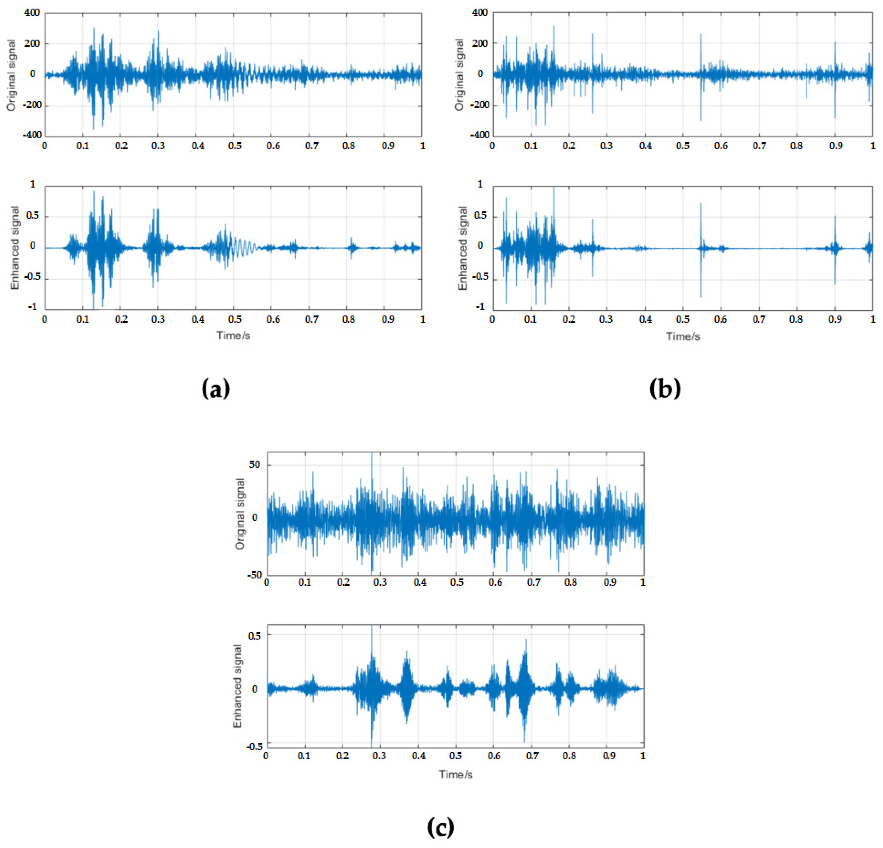
2.2. Spectral Subtraction

Whether in laboratory or factory environments, monitoring and fault diagnosis of crushers during equipment operation is always accompanied by environmental noise. Therefore, it is necessary to preprocess the sensor signals collected by spectral subtraction to reduce the signal interference.

As a stand-alone noise suppression algorithm, spectral subtraction is able to reduce the spectral effects of acoustically added noise in speech [25]. By subtracting an estimate of the noise spectrum from the noisy speech spectrum, an estimation of the clean speech signal spectrum can be obtained [26]. Generally, the estimation of the noise spectrum can be perceived during the no-load test before material feeding. According to the study reported in [27], the formula for spectral subtraction is as shown in Equation (1).

$$\begin{array}{l}letD\left(x\right)=P_s\left(x\right)-\alpha P_n\left(x\right)\\ P_s^{\prime }(x)=\{\begin{array}{l}D\left(x\right),ifD\left(x\right)>\beta P_n\left(x\right)\\ \beta P_n\left(x\right),otherwise\end{array}\\ with\alpha \ge 1,and0<\beta <<1\end{array}$$

(1)

where x is the input signal, $P_s^{\prime }\left(x\right)$ is the modified signal spectrum, $P_s\left(x\right)$ is the spectrum of the input noise-corrupted speech, $P_n\left(x\right)$ is the smoothed estimate of the noise spectrum, α is the subtraction factor and β is the spectral floor parameter. In this way, a great reduction in background noise can be achieved with very little effect on the intelligibility of the speech.

In recent years, spectral subtraction has been used widely in the field of sound source separation [28], fault detection [29], speaker identification [30], speech enhancement [29], encrypted speech [31], and random noise reduction [26].

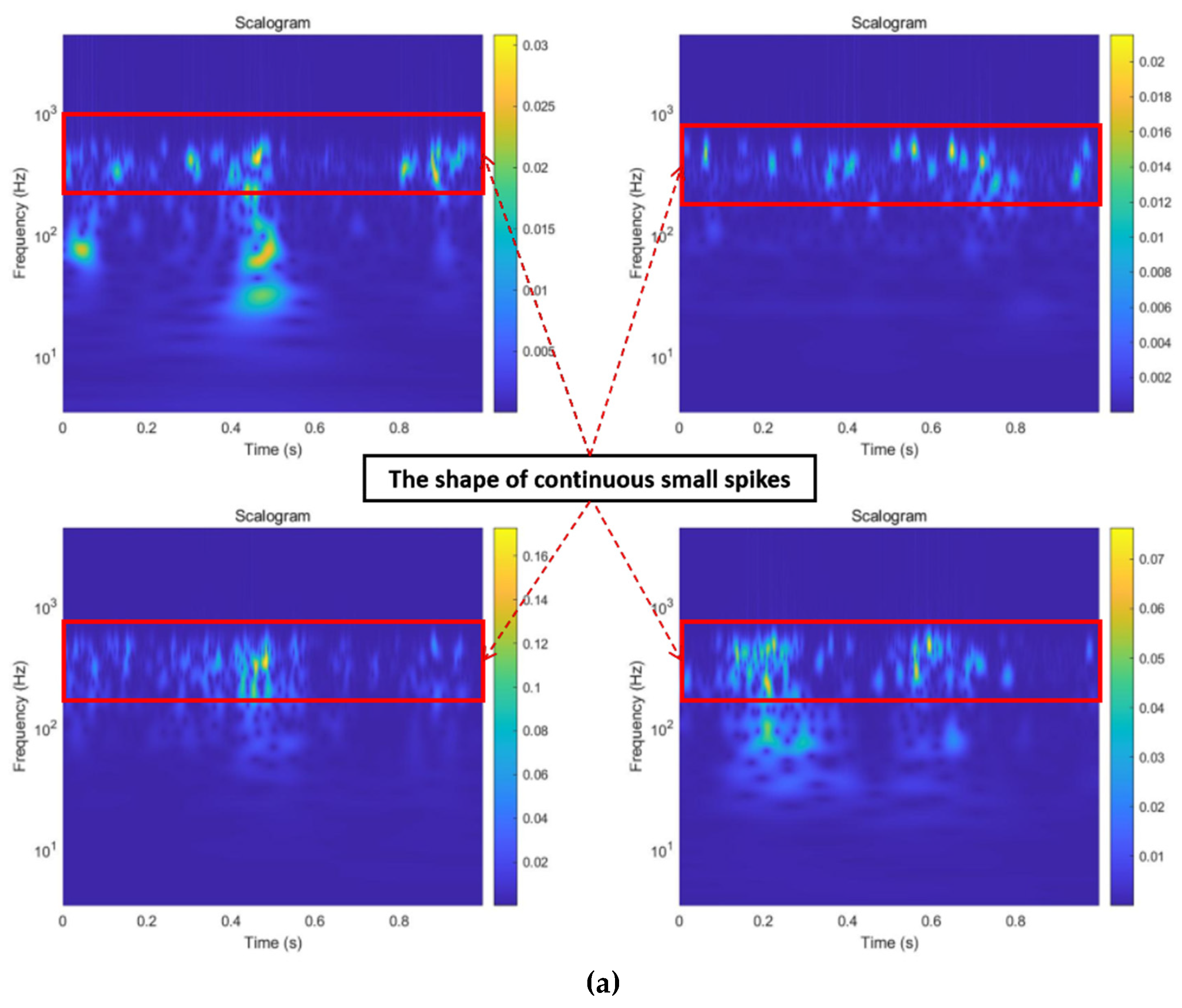
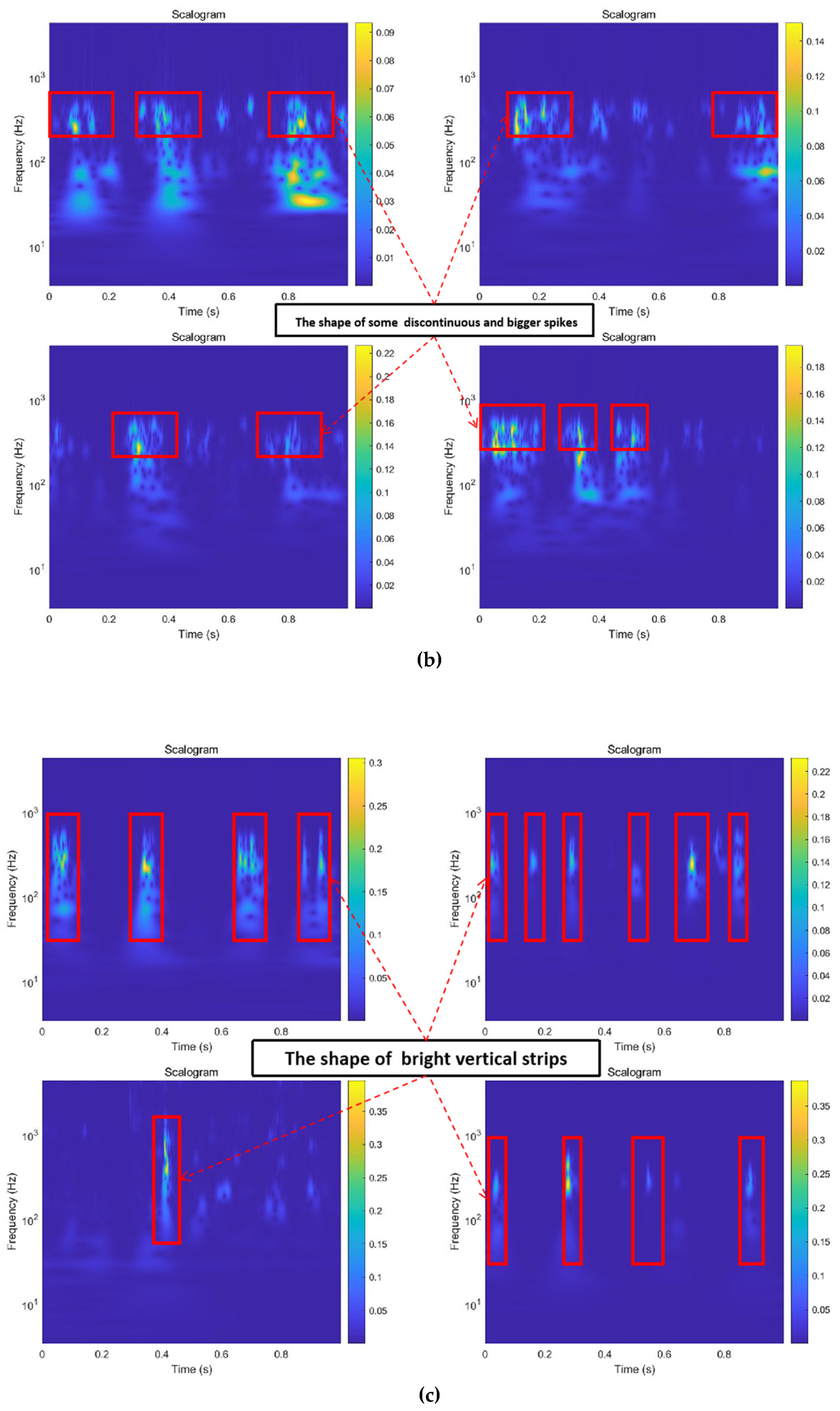
2.3. Continuous Wavelet Transforms

As a standard mathematical tool, wavelet transform (WT) is used for data analysis where features vary over different scales, and are primarily created to address the limitations of the Fourier Transform [32]. A base wavelet is needed in order to realize wavelet transform. The wavelet is a small wave that has an oscillating wavelike characteristic and has its energy concentrated in time. WT is based on decomposing signals into shifted and scaled versions of a wavelet and can be classified into two broad classes: the continuous wavelet transform (CWT) and the discrete wavelet transform (DWT) [33].

The CWT is a time–frequency transform, which is ideal for the analysis of non-stationary signals. Additionally, it can be used to analyze transient behavior, rapidly changing frequencies, and slowly varying behavior, which is very suitable for the research object of this article.

The CWT of a signal $x\left(t\right)$ is defined as shown in Equation (2) [34,35].

$$W_{\psi }\left(s,\tau \right)=\frac{1}{\sqrt{s}}{\displaystyle {\int }_{-\infty }^{\infty }x\left(t\right)}{\psi }^{\ast }\left(\frac{t-\tau }{s}\right)dt$$

(2)

where s represents the scale parameter, $\tau$ represents the time or translation parameter, $\psi (\cdot )$ represents the wavelet function with scale s and position offset $\tau$, and ${\psi }^{\ast }(\cdot )$ is the complex conjugate of $\psi (\cdot )$.

In this paper, the CWT is used to process vibration signals after spectral subtraction and to obtain the scalogram images, which correspond to the absolute value of the CWT coefficients of a signal.

2.4. Deep Learning and Convolutional Neural Networks

Nowadays, when it comes to problems of image recognition and classification, CNNs are regarded as the first choice for solving them [36]. Developed from machine vision, they are able to extract image features and build models automatically, overcoming the subjective influence of researchers. Moreover, they are able to improve on the accuracy and efficiency of image classification with the characteristics of weight sharing and local linking, and they have already been applied in image classification tasks in many fields, such as face recognition [37], iris recognition [38] in the biological field, license plate recognition [39] in the autonomous driving field, and to determine the concentrate ash content in coal flotation prediction [40], wet coal image classification [41], and in applications in the mining field.

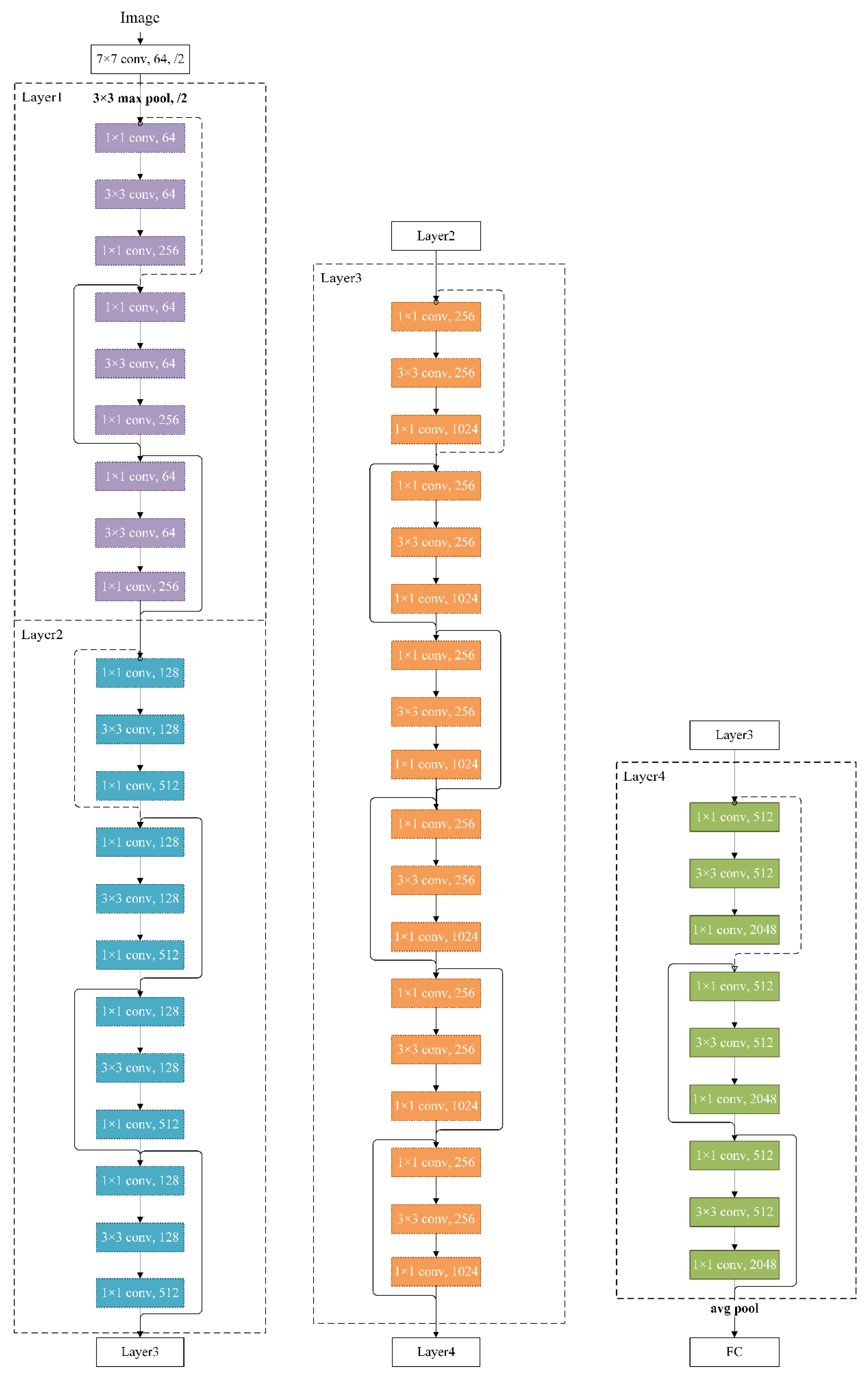
In particular, CNNs are a type of back propagation neural network with a deep structure that conducts classification tasks utilizing convolutional computation with translation invariance. Convolutional computation in the network can act as a substitute for fundamental matrix multiplication in CNNs.

CNNs primarily consist of input layers, convolutional layers, normalization layers, activation layers, pooling layers, fully connected layers, and a classification layer. In the network, different input and output layers are connected in parallel to capture image information, automatically update weights, and fulfill classification models. The specific composition is as follows:

(1) Input layers: This layer mainly pre-processes the original image data. In addition, mean-subtraction, normalization, PCA whitening, and local contrast normalization are some of the common pre-processing tools utilized. Because PCA whitening may enhance data noise, most CNN models just employ a basic mean-subtraction (and possibly normalization) step as a pre-processing step. The scaling and shifting accomplished by mean-subtraction and normalization are beneficial to gradient-based learning.

Specifically, mean-subtraction is used to make the mean value of the pixels at each position in all training images equal to zero. Given $N$ training images, where $x$ represents a single sample, the mean-subtraction step as shown in Equation (3).

$$x^{\prime }=x-\widehat{x}\begin{array}{cc},& \begin{array}{cc}where& \widehat{x}=\frac{1}{N}{\displaystyle \sum _{i=1}^N{x}_i}\end{array}\end{array}$$

(3)

where x represents the input signal, $N$ is the number of the input samples, and $i$ is an index.

The normalization function is employed so that the data will be at the same scale. To normalize the standard deviation to a unit value, the input data are divided by the standard deviation of each input dimension determined on the basis of the training set. This can be represented as shown in Equation (4).

$$x^{\prime }=\frac{x}{\sqrt{\frac{{\displaystyle {\sum }_{i=1}^N{\left(x_i-\widehat{x}\right)}^2}}{N-1}}}$$

(4)

where x represents the input signal, $N$ is the number of the input simples, and $i$ is an index.

(2) Convolutional layer: A convolutional layer is made up of a series of convolutional kernels, and each convolutional kernel can be regarded as a feature extractor. Different convolutional kernels extract different features in a complex way. The convolutional kernel is generally initialized in the form of a random decimal matrix, and reasonable weights are acquired in the process of training the network. The local receptive field is a region with the same size as the convolutional kernel in the input layer, and the convolutional result between the two is the value on a feature graph. The neuron of each convolutional layer usually contains several feature graphs, and the number of feature graphs is the depth of the convolutional kernel.

(3) Normalization layer: Batch normalization [42] is used to normalize the mean and variance of the output activations from a CNN layer so that it follows a unit Gaussian distribution [43]. The normalization of this distribution can be used to optimize the variance size and the mean position, and transfer the output value to the activation layer, which effectively improves the accuracy, prevents the gradient from disappearing or exploding, and accelerates network convergence. The batch normalization operation can be implemented as a layer in a CNN, as shown in Equation (5).

$$\begin{gathered} \widehat{x_i}=\frac{1}{{\sigma }_i}\left(x_i-{\mu }_i\right) \\ {y}_i=\gamma \widehat{x_i}+\theta \end{gathered}$$

(5)

where $x$ is the input of the layer, $i$ is an index, $\mu$ is the mean, $\sigma$ is the standard deviation, $\widehat{x_i}$ is the standard score, and $\lambda$ and $\theta$ are learnable variables.

(4) Activation layer: The activation function introduces a nonlinear factor to the neuron, meaning that the neural network can approach any nonlinear function arbitrarily, and thus the neural network can be applied to many nonlinear models. The Rectified Linear Unit (ReLU) activation function is the most commonly used activation function, due to its advantages of fast convergence speed, high efficiency, unilateral inhibition, relatively wide excited boundary, and better sparsity, as shown in Equation (6) [44].

$$\mathrm{ReLU}\left(x\right)=\max \left(x,0\right)=\{\begin{array}{c}0,x<0\\ x,x\ge 0\end{array}$$

(6)

(5) Pooling layer: the pooling layer in the middle of the continuous convolutional layer is able to compress data and reduce the number of parameters, thus reducing over-fitting, and can actually be considered to be a down-sampling operation. The commonly used pooling operations are max-pooling and average-pooling. Max-pooling can be defined as the selection of the largest element value from a locally related element set, while average-pooling is defined as the calculation of the average from a set of locally relevant elements, and returning it.

Briefly, max-pooling retains texture features, while average-pooling retains the overall data features. Therefore, max-pooling was selected in order to preserve more background information of the image and provide strong model robustness in this paper.

(6) Fully connected layer: The fully connection layer connects the features of all previous layers to form output values and transmits them to the classifier. In addition, it is actually the convolutional operation where the convolutional kernel size is equal to the upper feature size.

(7) Classification layer: The classification layer performs the final classification decision, and its main function is to output the probability that the object belongs to each class. For binary classification issues, the Sigmoid function is usually employed, as shown in Equation (7), while for multi-classification problems, the Softmax function is commonly utilized, as shown in Equation (8).

$$\mathrm{Sigmoid}\left(t\right)=\frac{1}{\left(1+e^{-t}\right)}$$

(7)

where $t$ is the output value, and the value range of Sigmoid is $(0,1)$.

$$\begin{array}{cc}\mathrm{Softmax}\left(p_i\right)=\frac{e^{p_i}}{{\displaystyle \sum _{k=1}^k{e}^{p_k}}},& i=1,\cdot \cdot \cdot ,m\end{array}$$

(8)

where $p_i$ is the output value, $k$ is the number of outputs, and the value range of Softmax is $\left[0,1\right]$.

In this paper, considering that the research object involves coal, wood, and iron, the Softmax function will be preferred. However, because the data analysis in the testing process also studies the dichotomy problem, the two functions need to be used separately. To realize the comparison of classification results, the Softmax function is selected for the final training classification.

2.5. Residual Neural Network

Residual Neural Network (ResNet) [45], which is extensively used in image classification, was chosen as the model for this experiment based on the scalogram classification of the feeding materials and the quantity of the feeding material image data.

The remarkable feature of the residual network architecture is the shortcut connection, as shown in Figure 1. When an input $x$ is given, the CNN weight layers implement a transformation function on this input, depicted by $F\left(x\right)$. In the residual blocks, the original input is added to this transformation using a direct connection from the input, which bypasses the transformation layers.

In ResNet, the layers are reformulated as learning residual functions with reference to the layer inputs, instead of learning unreferenced functions, and the results show that these residual networks are easier to optimize, and possess improved accuracy as a result of their considerable increase in depth [45,46,47]. Therefore, ResNet is widely used in image classification [48], image recognition [49], fault diagnosis [50], and so on.

2.6. Data Augmentation

When image classification is carried out by deep learning, a large amount of data is often needed to ensure the accuracy of the training results and to conduct deeper exploration and research on the classification mechanism. However, the feeding classification of double-toothed crushers faces the problem of an insufficient amount of data when conducting network training due to the low level of intelligence of the crushing equipment, the lower number of feeding signals obtained, and the lack of standard, unified and generalized open-source datasets.

One of the most common and effective ways of solving these problems is data augmentation [43]. Especially in cases where the number of training examples is relatively low, data augmentation can be used to enlarge the datasets to allow more robust training of large-scale models. Therefore, in the feeding material recognition task, this approach can be used to generate some new images by flipping, rotation, scaling, and clipping, with the aim of increasing the amount of data while preventing over-fitting [51].

3. Study Case

The experiment was divided into six parts, including sample preparation, signal acquisition, image transformation, datasets preparation, model development, and classification effect evaluation, as shown in Figure 2. Firstly, sample preparation involves sample type selection, quantity preparation, and size processing. Secondly, by putting the sample into the crusher, the sound pressure and vibration signals of different feeding materials are collected by the multi-sensor system. Thirdly, wavelet transform is applied to the original signals to produce scalograms, which represent the feeding feature images. Next, to develop the datasets, the picture of feeding characteristics is pre-processed for image augmentation. Then, the ResNet-50 model is utilized to establish the crusher feeding classification model, and the feeding characteristic images are trained and tested. Finally, the classification performance is analyzed and evaluated by using confusion matrix.

3.1. Experimental Settings

3.1.1. Sample Preparation

To collect signals during the crushing process of different kinds of materials, coal, wood and iron were selected as the normal material, interference material and harmful material, respectively. Furthermore, in this experiment, the coal sample used in this test was Taixi anthracite, and the wood used was common pine wood cubes. Considering the actual situation of industrial production with respect to the shape and size of the feeding materials, the feeding size was not strictly controlled, and this paper only gives an approximate size for statistical convenience. In this experiment, more attention was paid to the collected signals. Additionally, we used Q235B carbon steel to weld a hollow cylinder. The size of this cylinder was controlled not to be bitten, and it was able to bounce up and down slightly on the broken teeth in order to provide an impulse signal for iron entering the crushing chamber. Pictures of some materials are shown in Figure 3, and the measured quantity, size and mechanical properties of the aforementioned materials are shown in

Table 2. Physical and mechanical parameters of the feeding materials.

Sample	Taixi Coal	Pine	Q235B
Quantity	500	500	1
Size/mm	45~55	50 × 50 × 50	Φ 200 × 250 × 10
Density/g·cm−3	1.450	0.519	7.830
Tensile Strength/MPa	0. 953	102.8 (parallel to grain)	375~500
Elastic Modulus/MPa	3.40	16.30 (x)	210
		0.57 (y)
		1.10 (z)
Poisson Ratio	0.201	0.570 (xy)	0.274
		0.310 (yz)
		0.420 (xz)

.

For the determination of quantity and size, the approximate size was estimated with reference to the equipment parameters of the experimental crusher (which will be described in Section 3.1.2). Considering that the test was divided into single particle crushing and mixed crushing, and the number of samples required for training was large, we chose 500 groups of coal and wood. The mean and standard deviation of the validation validation accuracy for different sample sizes after 20 pre-tests are shown in

Table 3. The effect of training data size on the model performance.

Data Size	Mean Validation Accuracy	Standard Deviation
100	73.89%	2.6411
200	81.28%	2.1089
300	83.00%	1.4856
400	82.56%	0.8589
500	84.24%	0.5925
600	81.19%	0.9979

. Model classification performance was best when the data size was 500. According to the mechanical properties of coal, wood, and iron, it can be found that coal and wood are more similar to each other than to iron, while in terms of tensile strength and modulus of elasticity, iron is not on the same order of magnitude as the other two materials.

3.1.2. Test Device and Data Acquisition

The layout of the test system is shown in Figure 4, and includes three parts: the execution system, the acquisition system, and the processing system. The execution system includes a motor (1), a crushing gear roller (2), feeding materials (3), and other crusher components. The acquisition system is composed of the multi-sensor system and the data acquisition instrument (4), (5) and (6). The processing system includes the supporting software of the data acquisition instrument in the computer and the signal processing and analysis system for recognizing the feeding materials.

As shown in Figure 5, the main structure of the execution system is a ZKB-II shear crusher [52]. The motor current frequency is 30 Hz, and the motor speed is 864 r/min. In addition, the reduction ratio of the reducer is 71. The basic technical parameters of the machine are presented in

Table 4. The basic technical parameters of the ZKB-II shear crusher [52].

Technical Parameters	Value
Feed Size/mm	300 × 200 × 3
Product Particle Size/mm	20 × 20
Boundary Dimension/mm	1366 × 466 × 485
Operating Weight/kg	320
Maximum Current/a	6.8
Power/kw	3
Supply Voltage/v	380
Input Speed/r·min−1	1420

. The crushing materials for the test are single particles of coal, wood, and iron, respectively placed in the same position of the crusher in order to reduce interference from irrelevant variables.

So that the sample value would fully display the waveform variation law, a higher sampling frequency was necessary. The sampling frequency selected for this test was 10,240 Hz. A YSV 5000 IEPE sound pressure sensor with a sensitivity of 40 mV/Pa and a frequency response range of 20 Hz–20,000 Hz was selected to measure sound pressure. The sound pressure sensor was installed at the axial center line of the two crushing rollers, in order to avoid noise sources (such as motor, coupling, etc.) to the greatest extent possible. In addition, by means of voltage changes on the electret membrane in the sensor, the sound information of the feeding material during the working process is transmitted to the acquisition instrument. We selected two YA19T IEPE acceleration sensors with a sensitivity of 100 mV/g and a range of 50 g, and these were installed on the bearing seats at both ends of the crusher to guarantee the accuracy of the monitoring data. These sensors formed a multi-sensor system for monitoring and collecting sound and vibration signals during the feeding process of crushing. In addition, the YSV 8008 signal acquisition analyzer collected these signals to be stored in the computer. The system described above is the signal acquisition system.

3.1.3. Image Transformation

Due to the sample input requirements of CNNs, the collected data need to be transformed from one-dimensional signals into multidimensional images. The processing system was based on Python, which pre-processes the collected signals obtained from the crusher with different feeding materials by means of spectral subtraction, as shown in Figure 6, and subsequently carries out feature extraction of the denoising signals. In order to generate an image of the material that includes both sound and vibration signal characteristics, the commonly used method is to perform wavelet transform on the original signals.

In this paper, CWT was used to convert multidimensional signals, because it can be used to analyze transient behavior and describe the rapidly changing frequency characteristics, which are similar to those of the actual situation in industrial production. Specifically, the filter bank employs the analytic Morse (3,60) wavelet [53,54], which is intended for signals consisting of 10,240 samples. Furthermore, the size of the highest-frequency passband was set to be half of the peak value at the Nyquist frequency. The image transformation results from the sensor signals are shown in Figure 7.

By means of the above signal processing, the feature images and labels of three types of materials were obtained to be imported into the CNN for training and learning.

3.1.4. Dataset Preparation

After image transformation and data augmentation, a total of 560 coal images, 570 iron images, and 410 wood images were collected. In this experiment, data augmentation was only used in the image training set. In addition, the quantities of the training set, the validation set, and the test set were in the ratio 7:2:1.

Firstly, on the basis of what can be heard, the sound of coal feeding is relatively stable and low, while wood will produce a splitting sound in the process of crushing, and the sound of iron collision is loud and clear.

Secondly, as shown in Figure 6, the 1 s no-load signal was selected for spectral subtraction of the original signal, and the continuous signal was split into small segments with a time length of 1 s (considering the reaction time for monitoring the feeding material in production). The results show that in the time domain, the coal and wood amplitudes were close to 400, which is much larger than the amplitude of iron. On the basis of the waveform analysis, it can be observed that the iron signal has a certain periodicity, while the coal is more continuous, and the wood has an obvious spike.

According to Figure 7 and Figure 8, the scalogram of coal presents the shape of continuous small spikes, and the energy distribution extends over time, with most being in the range 100–1000 Hz, and the maximum energy can reach 0.16. Compared with coal, the scalogram of wood, with a similar frequency, is not continuous in time, and is in the shape of a bigger spike, which can be considered to be influenced by the differences in the physical and mechanical properties of wood in the horizontal and vertical directions. Under the same experimental conditions, the iron scalogram image is more obvious, forming a bright vertical strip and having high energy in the short time frequency distribution, because the collision between the iron and the crushing tooth within a very short time occurs at high frequency and generates a lot of energy, which can reach up to 0.35.

In summary, the feature pictures are able to reveal certain differences (e.g., time, frequency, energy, and waveform), thus providing the basis for image classification and recognition of feeding materials for crushers during subsequent operation.

3.2. Model Development

3.2.1. Model Building

For the feeding material image classification task, we built a 50-layer CNN model that was a variant variants of ResNet-50 [45,46]. It has 48 convolutional layers along with 1 max pool and 1 average pool layer.

This model is divided into 5 stages, as shown in Figure 9. The first stage has a relatively simple structure and can be regarded as the pre-processing of inputs. In addition, the last four stages are composed of bottlenecks and have similar structures.

Firstly, this model requires feature images that have a height, width, and channel of 224, 224 and 3, respectively. After a 3 × 3 zero padding, the results are entered into the pre-processing layer. In this layer, feature images are successively passed through the convolutional layer, the BN layer, the ReLU activation function, and the max pooling layer to obtain an output of 56 × 56 × 64. To be specific, the 2-D convolutional has 64 filters with dimensions of 7 × 7 and a convolutional kernel stride of 2. Additionally, the BN layer refers to batch normalization and max pooling using a 3 × 3 window and a 2 × 2 stride. In Layer 1, the convolutional block uses three sets of filters, and the numbers of 1 × 1, 3 × 3 and 1 × 1 filters are 64, 64 and 256, respectively. The two identity blocks also use three sets of filters, and the numbers of 1 × 1, 3 × 3 and 1 × 1 filters are 64, 64 and 256, respectively. In addition, Layers 2, 3 and 4 have the same structural principles as layer 1, and thus will not be described in detail in this paper, and the output size of layer 4 is 7 × 7 × 2080. Finally, 2-D average pooling is used to process the input features with window dimensions of 2 × 2, and through the fully connected layer and the Softmax layer, the input samples are classified and output.

In this experiment, the described models were developed, trained, and tested individually for the classifications of coal–iron–wood, coal–iron, and coal–wood, with model parameters as shown in

Table 5. Model Operation parameters.

Model	Input	Pooling Layer Active Function	Fully Connected Layer Active Function	Parameter	FLOPs
	224 × 224	ReLU	sigmoid	25.5 × 106	4.1 × 109

.

3.2.2. Implementation Setting Details

The model training environment and preset hyperparameters are shown in

Table 6. Training hyperparameters.

	Parameter Name	Selected Value
Optimization	Optimization name	SGDM
	Learning rate	1 × 10–3
	Momentum	0.9
	Loss function	Cross entropy loss
Fitting	Batch size	32
	Epochs	30
Environment	GPU	NVIDIA GeForce RTX 2060
	Platform	Python 3.8

.

The models used in this experiment were built based on Python 3.8 using Pytorch 1.10.0 toolbox. The Stochastic Gradient Descent Momentum (SGDM) optimizer was used in the model; the learning rate was 1 × 10^–3; the momentum was 0.9, and the loss function was cross-entropy loss. During training, the batch size was 32, and the number of epochs was 30. Additionally, the model was trained in NVIDIA GeForce RTX 2060 and CUDA 10.2, cudnn 8.0.2 environments.

3.3. Result Analysis

3.3.1. Model Evaluation

The accuracy and loss value of the CNN models for the feed feature images of different classification modes are shown in

Table 7. Accuracy and loss of CNN models.

Feed Materials	Train Loss	SD	Train Accuracy	SD	Valid Loss	SD	Valid Accuracy	SD
Coal, Wood & Iron	0.2271	0.0784	89.38%	5.4486	0.5925	0.0476	84.24%	0.6107
Coal & Iron	0.0002	0.0003	100%	0	0.2262	0.0337	93.78%	0.4464
Coal & Wood	0.2619	0.0816	84.69%	5.1254	0.5380	0.0630	80.07%	0.9597

, presented as the mean and standard deviation (SD) of 20 training results.

For the classification of coal, iron and wood, the model achieved a classification accuracy of 84.24%, which is not a very desirable training result. As a consequence, the classification of coal–iron and coal–wood needs to be further studied. According to the processing results, the model of coal–iron classification achieved an excellent classification accuracy of 93.78%. However, the model of coal–wood classification only achieved a classification accuracy of 80.07%, which was due to the lack of significant features for coal.

On the basis of previous studies in the literature [22], combined with the results of this experiment, it was assumed that this classification result was due to the fact that coal and wood are brittle materials compared to iron and are more easily destroyed in the crushing chamber; hence, the instantaneous crushing energy is more concentrated, whereas iron cannot be easily bitten into and only bounces periodically on the crushing teeth, which makes its characteristics more distinct than those of the other two incoming materials. In particular, as the physical and mechanical properties of coal and wood are more similar to each other, they could not be easily distinguished by means of a single feature, and additional classification features and sample sizes are required to further improve classification accuracy.

In summary, the classification performance of coal–iron was excellent, and was able to meet the production needs of crushers to monitor and minimize the presence of harmful iron, while the classification of coal, iron and wood was not very satisfactory due to the closer feeding characteristics of coal and wood, thus necessitating further exploration in future studies.

3.3.2. Confusion Matrix

The confusion matrix [55,56] was introduced as the evaluation index to more intuitively represent the classification of coal–iron, coal–wood, and coal–wood–iron in the CNN model, as well as to assess the misjudgment rate and the factors of misjudgment.

The confusion matrices of feeding datasets with different classified objects are shown in Figure 10, and the evaluation index of confusion matrix is shown in

Table 8. Evaluation index of confusion matrix.

Materials	Accuracy	Precision	Sensitivity	Specificity	F1-Score
Coal-Iron-Wood
Coal	84.0%	75.1%	86.3%	83.7%	80.3%
Iron		98.1%	88.3%	99.0%	92.9%
Wood		80.0%	74.8%	93.2%	77.3%
Coal-Iron
Coal	93.5%	88.8%	99.4%	87.7%	93.8%
Iron		99.3%	87.7%	99.4%	93.1%
Coal-Wood
Coal	80.1%	81.3%	85.1%	73.2%	83.2%
Wood		78.3%	73.2%	85.1%	75.7%

.

In Table 8, the accuracy is the proportion of all samples with correct predictions. Precision is the proportion of all outcomes predicted by the model as COAL, IRON or WOOD that were correct. Sensitivity is the proportion of all samples of COAL, IRON or WOOD that were correctly predicted by the model. Specificity is the proportion of all samples that were not COAL, IRON or WOOD that were correctly predicted by the model. In addition, F1-Score is defined as the harmonic average of precision and recall.

Firstly, the results show that the accuracy of the coal–iron–wood classification model was 84.0%. In terms of precision, the values of 75.1%, 98.1% and 80.0% for coal, iron and wood, respectively, indicate that the model predicted iron correctly at a higher rate. The sensitivity of coal, iron and wood was 86.3%, 88.3% and 74.8%, respectively, which shows that coal and iron were more easily detected compared to wood. Considering that the objective of the test was to remove harmful iron from the feed, further observation of the iron specificity and F1-Score suggests that the former indicates that the prediction accuracy for materials other than iron can reach up to 99.0%, while the latter indicates that the model has excellent classification performance for iron (the closer the indicator is to 100%, the better the classification performance).

Secondly, when the classification focus is placed on coal–iron, it can be found that the accuracy of the classification model can reach up to 93.5%, while the other four indicators were significantly improved compared with the first classification group, where it can be seen that the performance of the model was able to meet the needs of monitoring and discriminating iron in industrial production when only coal–iron was classified and identified. The reason the accuracy of the first group classification model was not high enough is most likely due to the mixing of wood, which leads to the low accuracy of coal and wood classification, and thus affects the overall performance index. In this paper, an attempt was made to test this hypothesis on the basis of coal–wood classification.

Finally, by comparing the coal–wood classification results, it can be concluded that the accuracy of coal–wood classification was not too high, at only 80.1%. This is because the material properties of coal and wood are relatively close to those of iron, and they can be easily broken in the crushing cavity, producing obvious sound and vibration signals, thus leading to the differentiability of the data signals collected during the test not being very high. In addition, the single selection of judging indicators and the lack of data volume may also be a reason for this observation. However, considering the small influence of wood entering the crusher, this was not further explored in this paper, and wood was only used as a disturbance term in coal–iron classification in order to test the accuracy and sensitivity of iron identification; a more in-depth study of this aspect will be conducted in future.

In summary, with the feature images and models selected in this paper, both in the classification of coal–iron–wood and in the classification of coal–iron, the classification accuracy of iron was very high, and was able to meet the realistic demands of monitoring and recognizing iron in the crushing chamber of crushers during industrial production, while the classification performance of coal and wood was not outstanding due to the similarity material properties, thus requiring further exploration and research in the future.

4. Conclusions

To exert its advantages and potential, image classification technology based on deep learning was applied to the field of mineral processing machinery in order to solve the problem of crushing equipment feed classification and to establish a system for status monitoring and fault diagnosis in crushing machine operation. In this paper, a CNN model was used to classify and judge different types of crushing feed material. First, the physical and crushing characteristics of different feed materials were investigated, and coal, iron, and wood were used as research objects. Secondly, the sound and vibration state signals of the crusher during the crushing of feed materials was obtained using signal acquisition equipment and processed by spectral subtraction and image transformation. Thirdly, different classification models were built for the three materials with the help of the ResNet of the CNN model to achieve the purpose of identifying the iron entering the crushing chamber. Finally, the classification model performance was evaluated using a confusion matrix to analyze the variability and the reason for the existence of different feeding feature images.

The detailed conclusions are as follows:

(1)

Referring to Resnet-50, the image classification model based on deep learning established in this experiment has good classification performance for typical crushing equipment feeding materials of. However, when wood was present in the classification object, the similarity between coal and wood led to a decrease in accuracy. The accuracies of coal–iron–wood classification, coal–iron classification and coal–wood classification obtained in this paper were 84.0%, 93.5% and 80.1%, respectively.

(2)

A comparative analysis of the three classification cases revealed that iron had higher precision, sensitivity, specificity, and F1-Score in the confusion matrix, indicating that the feeding characteristics of iron were more obvious than those of the other materials. In addition, coal–wood classification accuracy was lower, considering that due to their having similar mechanical properties and physical characteristics, and the fact that both are more likely to be crushed and generate large amounts of energy at the moment of crushing, these characteristics cannot be easily distinguished by a single indicator alone. The reason that this affects the accuracy of the three classifications lies in the fact that coal and wood cannot be easily separated.

(3)

To improve the accuracy of coal–wood classification, in-depth research based on increasing the number of feature indicators and the volume of data is needed in the future. Considering production demand, the accuracy of the current classification model is able to fully satisfy the purpose of excluding harmful iron from the crushing chamber and provide technical core support for the design of a system for crusher operating status monitoring and fault diagnosis. In the future, deep learning can be further combined with mineral engineering to try to explore the problems of mineral processing and machinery from a new perspective.

As the feeding identification of crushers is at a preliminary stage of exploration, there are still many limitations in current research. Firstly, the training data are not sufficient, and the training model can be further improved. Secondly, research on classification mechanisms needs further testing. In addition, the classification features of coal will be the focus of future study. In addition, an industrial test is required to verify the generalization of the model. In the future, we will carry out a study to build an intelligent communication and fault diagnosis system for mining machines, improving work efficiency and ensuring the safety of the production process.

References

1. Pan, Y. Development of China’s coal crushing equipment over the past 70 years and perspective. Coal Prep. Technol. 2019, 272, 32–36, 42. [Google Scholar] [CrossRef]
2. Lieberwirth, H.; Hillmann, P.; Hesse, M. Dynamics in double roll crushers. Miner. Eng. 2017, 103, 60–66. [Google Scholar] [CrossRef]
3. Zak, G.; Wylomanska, A.; Zimroz, R. Alpha-Stable Distribution Based Methods In The Analysis of The Crusher Vibration Signals For Fault Detection. Ifac Pap. 2017, 50, 4696–4701. [Google Scholar] [CrossRef]
4. Jha, P.K.; Rajora, R. Fault Diagnosis of Coal Ring Crusher in Thermal Power Plant: A Case Study. In Proceedings of the 2016 International Conference on Automatic Control and Dynamic Optimization Techniques (ICACDOT), Pune, India, 9–10 September 2016; pp. 355–360. [Google Scholar]
5. Liu, Q.; Song, B.; Ding, X.; Qin, S.J. Fault diagnosis of dynamic processes with reconstruction and magnitude profile estimation for an industrial application. Control Eng. Pract. 2022, 121, 105008. [Google Scholar] [CrossRef]
6. Obuchowski, J.; Zimroz, R.; Wylomanska, A. Identification of cyclic components in presence of non-Gaussian noise–Application to crusher bearings damage detection. J. Vibroeng. 2015, 17, 1242–1252. [Google Scholar]
7. Wylomanska, A.; Zimroz, R.; Janczura, J. Identification and stochastic modelling of sources in copper ore crusher vibrations. J. Phys. Conf. Ser. 2015, 628, 012125. [Google Scholar] [CrossRef] [Green Version]
8. Rahimdel, M.J.; Karamoozian, M. Fuzzy TOPSIS method to primary crusher selection for Golegohar Iron Mine (Iran). J. Cent. South Univ. 2014, 21, 4352–4359. [Google Scholar] [CrossRef]
9. Moshgbar, M.; Parkin, R.; Bearman, R.A. Application of fuzzy logic and neural network technologies in cone crusher control. Miner. Eng. 1995, 8, 41–50. [Google Scholar] [CrossRef]
10. Asbjörnsson, G.; Erdem, I.; Evertsson, M. Application of the Hilbert transform for diagnostic and control in crushing. Miner. Eng. 2020, 147, 106086. [Google Scholar] [CrossRef]
11. Wylomanska, A.; Zimroz, R.; Janczura, J.; Obuchowski, J. Impulsive Noise Cancellation Method for Copper Ore Crusher Vibration Signals Enhancement. IEEE Trans. Ind. Electron. 2016, 63, 5612–5621. [Google Scholar] [CrossRef]
12. Laha, S.K.; Swarnakar, B.; Kansabanik, S.; Uke, K.J. Rub-Impact Fault Diagnosis of a Coal Crusher Machine by Using Ensemble Patch Transformation and Empirical Mode Decomposition. In Nonstationary Systems: Theory and Applications; Springer: Cham, Switzerland, 2022; pp. 265–278. [Google Scholar]
13. Sun, Y.H.; Li, C.; Huang, M.F.; Jing, H. Garbage Crusher Fault Diagnosis Based on RBF Neural Network. Appl. Mech. Mater. 2009, 16, 971–975. [Google Scholar] [CrossRef]
14. Li, X.; Li, C.; Huang, M.; Jing, H. The Fault Diagnosis of Garbage Crusher Based on Ant Colony Algorithm and Neural Network. In Proceedings of the 2009 Third International Conference on Genetic and Evolutionary Computing, Guilin, China, 14–17 October 2009; pp. 515–519. [Google Scholar]
15. Ma, L.C.; Zhang, Y.; Lv, P.; Ca, F.; Liu, Y.H. Research on Fault Diagnosis System of Crusher Based on BP Neural Network. In Proceedings of the 2020 Chinese Control And Decision Conference (CCDC), Hefei, China, 22–24 August 2020; pp. 677–682. [Google Scholar]
16. Olivier-Maget, N.; Negny, S.; Hetreux, G.; Le Lann, J.M. Fault diagnosis and process monitoring through model-based and case based reasoning. Comput-Aided Chem. Eng. 2009, 26, 345–350. [Google Scholar]
17. Park, S.; Jung, D.; Nguyen, H.; Choi, Y. Diagnosis of Problems in Truck Ore Transport Operations in Underground Mines Using Various Machine Learning Models and Data Collected by Internet of Things Systems. Minerals 2021, 11, 1128. [Google Scholar] [CrossRef]
18. Li, H.; Asbjörnsson, G.; Lindqvist, M. Image Process of Rock Size Distribution Using DexiNed-Based Neural Network. Minerals 2021, 11, 736. [Google Scholar] [CrossRef]
19. Jia, L.; Yang, M.; Meng, F.; He, M.; Liu, H. Mineral Photos Recognition Based on Feature Fusion and Online Hard Sample Mining. Minerals 2021, 11, 1354. [Google Scholar] [CrossRef]
20. Iwaszenko, S.; Róg, L. Application of Deep Learning in Petrographic Coal Images Segmentation. Minerals 2021, 11, 1265. [Google Scholar] [CrossRef]
21. Chow, B.; Reyes-Aldasoro, C. Automatic Gemstone Classification Using Computer Vision. Minerals 2021, 12, 60. [Google Scholar] [CrossRef]
22. Pan, Y.; Li, Z.; Zhu, C.; Liu, W.; Lang, J.; Wei, Y.; Yao, F.; Liu, Z. Research on the fault diagnosis of coal preparation equipment based on Artificial Neural Networks. In Proceedings of the XIX International Coal Preparation Congress, New Delhi, India, 13 November 2019. [Google Scholar]
23. Chen, X. Research on Fault Identification System of Crusher Based on Signal Analysis and Convolution Neural Network. Master’s Thesis, China University of Mining & Technology, Beijing, China, 2021. [Google Scholar]
24. Yan, Y. Research on Breaker Fault Identification Technology Based on Audio Signal Analysis. Master’s Thesis, China University of Mining & Technology, Beijing, China, 2020. [Google Scholar]
25. Boll, S. Suppression of acoustic noise in speech using spectral subtraction. IEEE Trans. Acoust. Speech Signal Process. 1979, 27, 113–120. [Google Scholar] [CrossRef] [Green Version]
26. Hao, L.; Cao, S.; Zhou, P.; Chen, L.; Zhang, Y.; Li, K.; Xie, D.; Geng, Y.; Cavaleri, L. Denoising Method Based on Spectral Subtraction in Time-Frequency Domain. Adv. Civ. Eng. 2021, 2021, 1–12. [Google Scholar] [CrossRef]
27. Berouti, M.; Schwartz, R.; Makhoul, J. Enhancement of speech corrupted by acoustic noise. In Proceedings of the Acoustics, Speech, and Signal Processing, IEEE International Conference on ICASSP ’79, Washington, DC, USA, 2–4 April 1979. [Google Scholar]
28. Ozawa, K.; Morise, M.; Sakamoto, S.; Watanabe, K. Sound Source Separation by Spectral Subtraction Based on Instantaneous Estimation of Noise Spectrum. In Proceedings of the 2019 6th International Conference on Systems and Informatics (ICSAI), Shanghai, China, 2–4 November 2019; pp. 1137–1142. [Google Scholar]
29. Yan, X.; Yang, Z.; Wang, T.; Guo, H. An Iterative Graph Spectral Subtraction Method for Speech Enhancement. Speech Commun. 2020, 123, 35–42. [Google Scholar] [CrossRef]
30. Siam, A.I.; El-khobby, H.A.; Elnaby, M.M.A.; Abdelkader, H.S.; El-Samie, F.E.A. A Novel Speech Enhancement Method Using Fourier Series Decomposition and Spectral Subtraction for Robust Speaker Identification. Wirel. Pers. Commun. 2019, 108, 1055–1068. [Google Scholar] [CrossRef]
31. Zhang, Q.-y.; Li, G.-l.; Huang, Y.-b. An efficient retrieval approach for encrypted speech based on biological hashing and spectral subtraction. Multimed. Tools Appl. 2020, 79, 29775–29798. [Google Scholar] [CrossRef]
32. Stark, H.-G. Continuous wavelet transform and continuous multiscale analysis. J. Math. Anal. Appl. 1992, 169, 179–196. [Google Scholar] [CrossRef] [Green Version]
33. Shi, Y.; Ruan, Q. Continuous wavelet transforms. In Proceedings of the 7th International Conference on Signal Processing, ICSP ’04, Beijing, China, 31 August–4 September 2004; Volume 201, pp. 207–210. [Google Scholar]
34. Yuan, L.; Lian, D.; Kang, X.; Chen, Y.; Zhai, K. Rolling Bearing Fault Diagnosis Based on Convolutional Neural Network and Support Vector Machine. IEEE Access 2020, 8, 137395–137406. [Google Scholar] [CrossRef]
35. Rioul, O.; Vetterli, M. Wavelets and signal processing. IEEE Signal Process. Mag. 1991, 8, 14–38. [Google Scholar] [CrossRef] [Green Version]
36. LeCun, Y.; Bengio, Y.; Hinton, G. Deep learning. Nature 2015, 521, 436–444. [Google Scholar] [CrossRef] [PubMed]
37. Deng, J.; Guo, J.; Xue, N.; Zafeiriou, S. ArcFace: Additive Angular Margin Loss for Deep Face Recognition. In Proceedings of the 2019 IEEE/CVF Conference on Computer Vision and Pattern Recognition (CVPR), Long Beach, CA, USA, 15–20 June 2019; pp. 4685–4694. [Google Scholar]
38. Daugman, J. How Iris Recognition Works. IEEE Trans. Circuits Syst. Video Technol. 2004, 14, 21–30. [Google Scholar] [CrossRef]
39. Chang, S.L.; Chen, L.S.; Chung, Y.C.; Chen, S.W. Automatic License Plate Recognition. IEEE Trans. Intell. Transp. Syst. 2004, 5, 42–53. [Google Scholar] [CrossRef]
40. Wen, Z.; Zhou, C.; Pan, J.; Nie, T.; Jia, R.; Yang, F. Froth image feature engineering-based prediction method for concentrate ash content of coal flotation. Miner. Eng. 2021, 170, 107023. [Google Scholar] [CrossRef]
41. Liu, Y.; Zhang, Z.; Liu, X.; Wang, L.; Xia, X. Performance evaluation of a deep learning based wet coal image classification. Miner. Eng. 2021, 171, 107126. [Google Scholar] [CrossRef]
42. Ioffe, S.; Szegedy, C. Batch Normalization: Accelerating Deep Network Training by Reducing Internal Covariate Shift. In Proceedings of the 32nd International Conference on International Conference on Machine Learning, Lille, France, 6–11 July 2015; pp. 448–456. [Google Scholar]
43. Salman, K.; Hossein, R.; Syed Afaq Ali, S.; Mohammed, B.; Gerard, M.; Sven, D. A Guide to Convolutional Neural Networks for Computer Vision; Morgan & Claypool: San Rafael, CA, USA, 2018; p. 1. [Google Scholar]
44. Jarrett, K.; Kavukcuoglu, K.; Ranzato, M.; LeCun, Y. What is the best multi-stage architecture for object recognition? In Proceedings of the 2009 IEEE 12th International Conference on Computer Vision, Kyoto, Japan, 29 September–2 October 2009; pp. 2146–2153. [Google Scholar]
45. He, K.; Zhang, X.; Ren, S.; Sun, J. Deep Residual Learning for Image Recognition. In Proceedings of the 2016 IEEE Conference on Computer Vision and Pattern Recognition (CVPR), Las Vegas, NV, USA, 27–30 June 2016. [Google Scholar]
46. He, K.; Zhang, X.; Ren, S.; Sun, J. Delving Deep into Rectifiers: Surpassing Human-Level Performance on ImageNet Classification. In Proceedings of the CVPR, Boston, MA, USA, 7–12 June 2015. [Google Scholar]
47. Wu, Z.; Shen, C.; Hengel, A. Wider or Deeper: Revisiting the ResNet Model for Visual Recognition. Pattern Recognit. 2019, 90, 119–133. [Google Scholar] [CrossRef] [Green Version]
48. Ma, L.; Shuai, R.; Ran, X.; Liu, W.; Ye, C. Combining DC-GAN with ResNet for blood cell image classification. Med. Biol. Eng. Comput. 2020, 58, 1251–1264. [Google Scholar] [CrossRef] [PubMed]
49. Razavi, M.; Alikhani, H.; Janfaza, V.; Sadeghi, B.; Alikhani, E. An Automatic System to Monitor the Physical Distance and Face Mask Wearing of Construction Workers in COVID-19 Pandemic. SN Comput. Sci. 2022, 3, 27. [Google Scholar] [CrossRef] [PubMed]
50. Zhao, M.; Zhong, S.; Fu, X.; Tang, B.; Pecht, M. Deep Residual Shrinkage Networks for Fault Diagnosis. IEEE Trans. Ind. Inform. 2020, 16, 4681–4690. [Google Scholar] [CrossRef]
51. Shorten, C.; Khoshgoftaar, T.M. A survey on Image Data Augmentation for Deep Learning. J. Big Data 2019, 6, 60–108. [Google Scholar] [CrossRef]
52. Zhou, C.; Pan, Y.; Lu, M. ZKB shear breaker and analysis on its performance. Coal Prep. Technol. 2004, 6, 21–23. [Google Scholar]
53. Olhede, S.C.; Walden, A.T. Generalized Morse wavelets. IEEE Trans. Signal Process. 2002, 50, 2661–2670. [Google Scholar] [CrossRef] [Green Version]
54. Lilly, J.M.; Olhede, S.C. Generalized Morse Wavelets as a Superfamily of Analytic Wavelets. IEEE Trans. Signal Process. 2012, 60, 6036–6041. [Google Scholar] [CrossRef] [Green Version]
55. Charles, E.M. Basic principles of ROC analysis. Semin. Nucl. Med. 1978, 8, 283–298. [Google Scholar] [CrossRef]
56. Fawcett, T. An introduction to ROC analysis. Pattern Recognit. Lett. 2006, 27, 861–874. [Google Scholar] [CrossRef]
Figure 1. The typical structure of ResNet.
Minerals 12 00380 g001
Figure 2. Flow diagram of experiment.
Minerals 12 00380 g002
Figure 3. The feeding materials. (a) Taixi coal; (b) pine cube; (c) Q235B hollow cylinder.
Minerals 12 00380 g003
Figure 4. Schematic diagram of test system. (1—motor, 2—crushing gear roller, 3—feeding materials, 4—acceleration sensor, 5—sound pressure sensor, and 6—signal acquisition system).
Minerals 12 00380 g004
Figure 5. ZKB-II shear breaker.
Minerals 12 00380 g005
Figure 6. Enhanced signals of (a) coal, (b) wood, and (c) iron.
Minerals 12 00380 g006
Figure 7. Segments of feature images from (a) sound pressure signal, (b) vibration signal 1, and (c) vibration signal 2.
Minerals 12 00380 g007
Figure 8. The typical feature images of (a) coal, (b) wood, and (c) iron.
Minerals 12 00380 g008aMinerals 12 00380 g008b
Figure 9. Experimental model architecture.
Minerals 12 00380 g009
Figure 10. Confusion matrices of (a) coal–iron–wood classification, (b) coal–iron classification, and (c) coal–wood classification.
Minerals 12 00380 g010aMinerals 12 00380 g010b