Estimating Residence Time Distributions in Industrial Closed-Circuit Ball Mills

Abstract

This paper compares two deconvolution methodologies used to estimate residence time distributions (RTD) in industrial closed-circuit ball mills. Parametric and non-parametric deconvolution techniques were evaluated. Both techniques allowed for direct RTD estimates from inlet and outlet tracer measurements in the mills, with no need for mass balances nor assumptions to correct the effect of the tracer recirculation in the grinding circuits. Measurements of inlet and outlet concentrations were conducted by radioactive solid tracers and on-stream detectors. The parametric deconvolution was applied assuming the N-perfectly-mixed-reactors-in-series model, whereas the non-parametric deconvolution consisted of a constrained least squares estimation subject to non-negativity. The shapes of the estimated RTDs were consistent between these methodologies, showing mound-shaped distributions in all cases. From the parametric approach, mixing regimes described by 2–4 perfect mixers in series were observed, which indicated significant differences regarding perfect mixing. The mean (τ_mean) and median (τ₅₀) residence times were more consistent with the RTD shapes when applying the parametric deconvolution. The non-parametric approach was more sensitive to noise, a disadvantage leading to mean residence times significantly higher than the median, and less consistent with the RTD locations. From the comparisons, the estimation strategies proved to be applicable in industrial closed-circuit ball mills. The parametric deconvolution led to better overall performances for τ₅₀ = 1.7–8.3 min, given a suitable model structure for the RTDs.

1. Introduction

Ball mills are widely used in mineral processing due to their flexibility and versatility in reducing the particle size at the level required in the concentration stages [1]. The size reduction can be carried out in dry or wet environments depending on the subsequent separation processes [2]. Grinding circuits must guarantee adequate particle size distributions and mineral liberations for the successful performance in the concentration circuits [3]. As grinding is intensive in energy consumption, significant improvements in the overall process efficiency can be achieved by approaching optimal conditions in ball mill operations [4].

The degree of grinding depends on the types of ores and several operating variables. One of these variables being the time that the particles remain inside the mill, which is a key factor in obtaining an adequate degree of liberation, keeping over-grinding under control. Too short solid residence times in the mill typically result in coarse products and poor liberation, whereas too long residence times favor over-grinding that also decreases the energy efficiency [1]. Thus, the characterization of the mean residence time and the residence time distribution (RTD) are critical to obtain adequate particle size distributions for concentration, minimizing the energy consumption per ton of ore [5].

Various studies have reported residence time distributions in ball mills, evaluating different phases (liquid and solid tracers), grinding circuits (open and closed circuits), and scales (laboratory, pilot, and industrial mills) [2,6,7,8,9,10,11]. Industrial characterization has been rather scarce. Mori, Jimbo and Yamazaki [9] determined ball mill RTDs at laboratory and pilot scales, in which grinding was operated in an open circuit. Copper sulfate was used as a tracer. The RTDs were adequately represented by a logarithmic-normal distribution, which included a dispersion parameter related to the level of mixing. A theoretical model was also derived, allowing the mixing regime to be evaluated from a diffusion coefficient. Kelsall, Reid and Restarick [6] presented RTD measurements for liquid and solid tracers in a laboratory scale ball mill under different experimental conditions. NaCl was used as a liquid tracer, and unbreakable particles and breakable minerals were used as solid tracers in a continuous open-circuit system. The RTD shapes showed low sensitivity to changes in the operating conditions; however, a residence time increase was attributed to an induced hold-up weight increase. The difficulties in the tracer injection to produce perfect impulses (for liquid tracer) or steps (for solid tracers) were highlighted. Any deviations regarding perfect injections were assumed negligible with respect to the mill residence time. The RTDs were modelled by a perfect mixer with a transport delay. Makokha, Moys and Bwalya [10], Makokha and Moys [2] and Makokha, Madara, Namago and Ataro [11] conducted RTD measurements in an industrial open-circuit ball mill, employing sodium chloride as a tracer. Different model structures were used to describe the ball mill RTDs and slurry transport, including a mixing model to represent the in-mill grinding performance and two macroscopic RTD models consisting of multi-stirring stages plus dead times. All models adequately fitted the experimental data. Gupta and Patel [7] modelled RTD data from ball and rod mills reported in the literature [12,13,14], showing that the RTDs were adequately represented as a sequence of perfect mixers arranged from the largest to the smallest in a geometric progression. A one-parameter model was used to represent this progression. The measurements involved different experimental conditions and grinding schemes. The studied datasets [12,13,14] considered different strategies to determine RTDs in ball mills in the presence of tracer recirculation (from the hydrocyclone underflow). The methodologies involved mass balances in the circuits or a multistage system identification (hydrocyclones, pipelines and sump box) to remove the effect of the tracer recirculation on the outlet tracer concentrations. Both approaches have been typically used when the RTDs are estimated from a single concentration measurement in the outlet stream of the ball mills. Hassanzadeh [8] measured liquid RTDs in an industrial ball mill operated in closed circuit with hydrocyclones. An aqueous NaCl solution was employed as a liquid tracer. Although the RTDs were adequately modelled by two perfect mixers in series plus a dead time, no corrections were made to account for the tracer recirculation in the mill-hydrocyclone system.

Since the pioneering work conducted by Gardner et al. [15], several studies have used radioactive tracers to characterize mixing regimes in ball mills [12,13,14]. For example, Marchand, Hodouin and Everell [12] employed tritiated water to measure RTDs in an industrial closed-circuit ball mill. The RTDs were corrected taking the tracer recirculation into consideration. Thus, mass balances were conducted in the grinding circuit, and a tracer delay from the mill discharge to the feed was used to compensate the activity signals. This approach assumed no mixing in the sump box, hydrocyclones and pipelines. Rogers, Bell and Hukki [13] studied ball mill RTDs, for closed-circuit operations with classifiers. The radioactive tracer technique was employed, using the short-lived radioactive tracer (SLRT) methodology proposed by Gardner, Rogers and Verghese [15]. Only one detector was installed in the outlet stream of the ball mill. Therefore, fine particles were traced such that the recycling fraction was determined from the hydrocyclone performance inefficiency. In addition, assumptions on the pipeline, sump box and hydrodyclone RTDs were necessary to correct the measured activity. Austin, Rogovin, Rogers and Trimarchi [14] measured ball mill RTDs at laboratory and pilot scales, also using the SLRT method reported in [15]. Both mills were operated in open circuit. Detectors were installed along the outside of the mills and in the grinding product; however, the inlet signals were not measured. The results showed that the RTDs were compatible with those predicted by the axial mixing model with a dimensionless mixing factor not dependent on particle size. Yianatos et al. [16] measured ball mill RTDs at industrial scale. The mill was operated in closed circuit with hydrocyclones. The radioactive tracer technique was used for the liquid phase, with only one detector installed in the outlet stream of the mill. The inlet activity was reconstructed, assuming that 38% of the outlet tracer was recirculated to the feed (obtained from mass balances), with a transport delay of 20 s (from estimated residence times in the pipelines and hydrocyclone racks). Thus, the ball mill RTDs were obtained from the deconvolution of the outlet activity and the reconstructed tracer feed. No details on the deconvolution algorithm were reported.

Table 1. Summary of the most relevant RTD studies on ball mills.

Scale	Circuit	Mill Diameter, m	Mill Length, m	RTD Identification
Laboratory [6]	Open	0.305	0.153–0.458	A perfect injection was assumed, estimating the RTDs directly from the outlet tracer concentrations
Laboratory [9]	Open	0.254	0.495	A perfect injection was assumed, estimating the RTDs directly from the outlet tracer concentrations
Laboratory [14]	Open	0.305	0.61	A perfect injection was assumed, estimating the RTDs directly from the outlet tracer concentrations
Pilot [9]	Open	0.545	1.98	A perfect injection was assumed, estimating the RTDs directly from the outlet tracer concentrations
Pilot [13]	Open	0.91	1.53	A perfect injection was assumed, estimating the RTDs directly from the outlet tracer concentrations
Pilot [13]	Closed	0.91	1.53	No inlet detection. Negligible tracer dispersions in the classifier and recycle loop were assumed; therefore, a time delay was considered for the tracer recycled to the mill feed. Independent RTD measurements in the sump box. RTDs were estimated by reconstructing the outlet tracer concentration, taking all mixing stages and assumptions into consideration.
Pilot [14]	Open	0.91	1.52	A perfect injection was assumed, estimating the RTDs directly from the outlet tracer concentrations
Pilot [15]	Open	0.406	0.813	A perfect injection was assumed, estimating the RTDs directly from the outlet tracer concentrations
Pilot [15]	Closed	0.406	0.813	No deconvolution procedure was specified
Industrial [2,10,11]	Open	7.31	9.6	A perfect injection was assumed, estimating the RTDs directly from the outlet tracer concentrations
Industrial [8]	Closed	5.03	8.23	No deconvolution procedure was specified
Industrial [12]	Closed	2.74	3.66	From mass balances, the hydrocyclone water split coefficient and the water flowrates through the mill were estimated. Time delays between mill discharge and the mill feed were obtained from the differences in the tracer peaks from the mill discharge to the hydrocylone underflow, assuming plug flows in the pump, sump and pipelines. Time delay corrections to obtain the ball mill RTDs, similar to an open circuit experiment.
Industrial [16]	Closed	3.05	4.27	No inlet detection. Mass balances to obtain the water recirculation to the mill. Estimations of time delays to approximate the residence time in the hydrocyclone racks and piping. Average residence time in the sump was estimated considering the box volume, typical filling levels, feed flowrates and solid percentages. Tracer feed reconstruction, calculated as the initial impulse plus an estimated tracer recirculation with a transport delay.
Laboratory–Pilot–Industrial [7]	Analysis of RTD data from previous studies, including different scales, mill sizes, experimental procedures and estimation strategies.

summarizes the most relevant RTD studies on ball mills, detailing the scales, machine sizes, circuit configurations and identification techniques.

Ideal tracer injections (Dirac delta impulses) allow the RTDs to be directly obtained from the outlet tracer concentrations. Due to the circulating load, the inlet signals differ from ideal impulses in closed-circuit ball mills. Deconvolution techniques are then required to obtain RTDs in ball mills. From literature, different strategies to correct non-ideal injections have been proposed: (i) assumptions on the RTD of all circuit components to decouple the ball mill RTDs; (ii) mass balances around the classifiers to quantify the tracer recirculation; and (iii) transport delay assumptions throughout the circuit to estimate the actual inlet concentrations. All these strategies implicitly and indirectly involve RTD identification by deconvolution. This paper compares two direct deconvolution techniques to estimate ball mill RTDs in industrial closed circuits: a parametric and a non-parametric deconvolution. These techniques do not require mass balances nor additional RTD assumptions to characterize closed-circuit ball mills. Radioactive tracers (for solids) along with online detectors were used to obtain the inlet and outlet signals. The agreements between the RTD estimates are discussed in terms of the RTD shapes, and the mean and median residence times in the evaluated ball mills.

2. Experimental Procedure

An industrial grinding circuit consisting of three semi-autogenous (SAG) lines was studied. Each line involves SAG and ball mill–hydrocyclone stages to obtain the particle size required in the flotation feed, P₈₀ ~ 200 μm. The circuit processes approximately 8000 tph of a copper ore, with typical Cu feed grades of 0.6%. Ball mills 1, 2 and 3 from two SAG lines were tested to estimate the residence time distributions by radioactive tracer experiments. 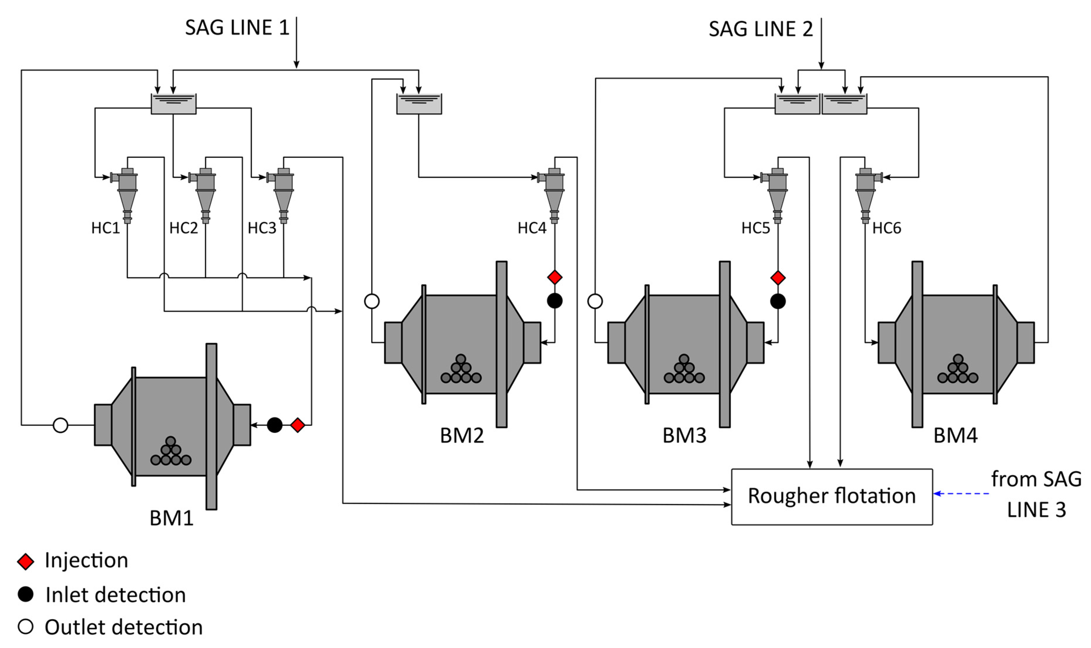Figure 1 presents a schematic of the SAG lines 1 and 2. Each line involves 11 m × 5.2 m SAG mills. Line 1 includes two 6.4 m × 10.2 m ball mills (BM1 and BM2, respectively), whereas Line 2 includes one 9.1 m × 13.7 m ball mill and one 6.4 m × 10.2 m ball mill (BM3 and BM4, respectively). Classification racks consist of fourteen 0.84-m diameter hydrocyclones. The overall product of the SAG lines (hydrocyclone overflows) feeds the rougher flotation circuit. For further details on the process diagram, please refer to [17]. The secondary grinding circuits typically present circulating loads ranging from 400% to 550% [17]. In the tracer tests, the maximum relative standard deviation of the feed flowrates to the SAG lines was 7.6%. The ball and pulp filling levels in the ball mills (by volume) were estimated at about 28%–34% and 12%–14%, respectively.

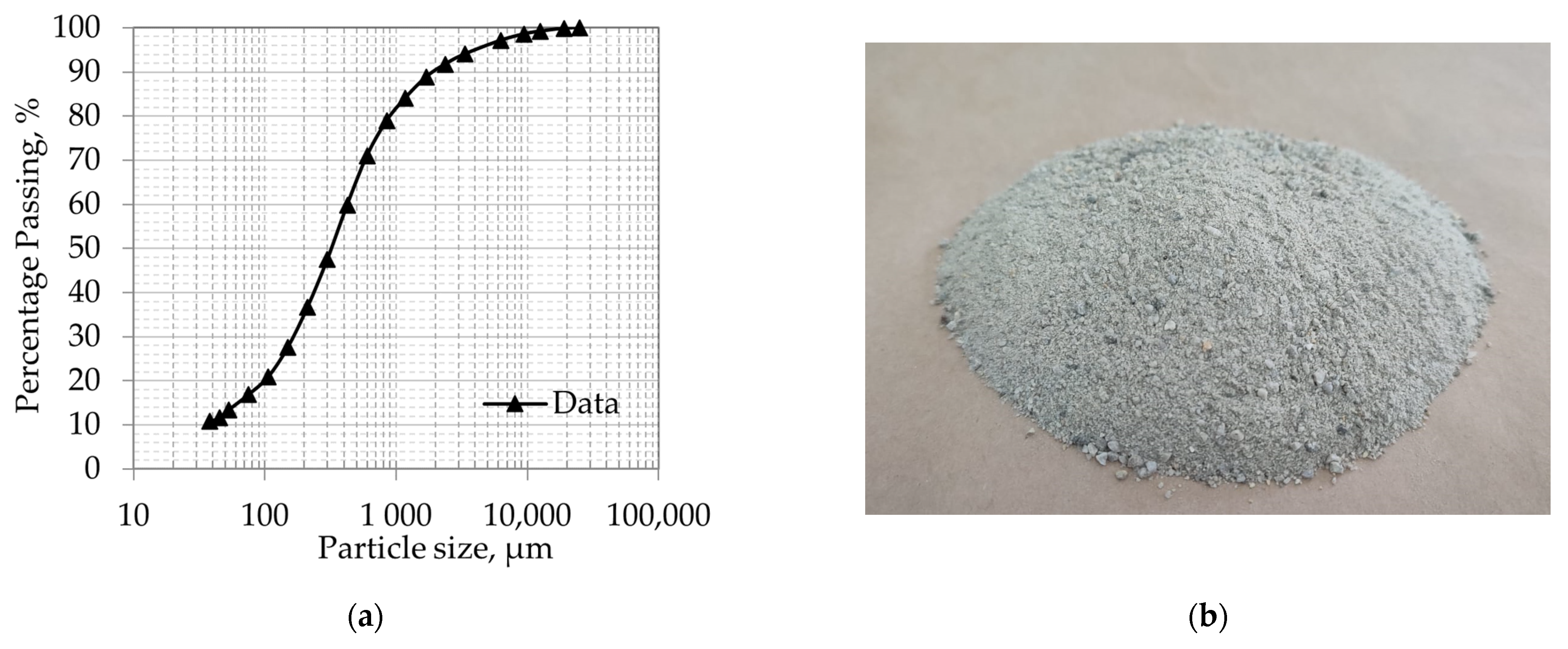
Three tracer experiments were performed in the ball mills BM1, BM2 and BM3 by tracer injection at each inlet stream. Injection and detection points are depicted in Figure 1. To keep the physical and chemical properties of the solid fed to the mills, dry samples from the underflow of the hydrocyclones were previously taken from the industrial circuit to be employed as solid tracers. Appendix A presents the average particle size distribution of these samples. The solid was activated in the RECH-1 nuclear reactor at La Reina Nuclear Centre, in Santiago, Chile. Thus, the activated samples mimicked the solids fed to the ball mills in the industrial tests. Radioactivity type and intensity were determined taking the flow rates and pulp characteristics into consideration, allowing for real-time measurements [18]. The solid samples were chemically assayed for element detection to produce radioisotopes by gamma neutron activation. The activated component was Na²⁴ for these samples. The tracer activity was set to 15 mCi, which was contained in c.a. 15–30 g of solids. A neutronic flux of up to 5 $\times$ 10¹³ n/cm² spatially homogeneous in 4$\pi$ was used for irradiation. The samples were placed inside a grid with the combustible elements exposed to the flux for homogeneous activation. Samples were submitted to the neutronic flux for approximately 20 h to provide significant activity (c.a. 50 times) above typical local backgrounds. The mean lifetime of the activated tracer was approximately 15 h. The tracer injection was carried out by introducing 100 mL of tracer in the inlet stream, using a hydraulic system that guaranteed an almost instantaneous, simple, and safe injection. As a result, the pulse signal approached an impulse in time and space, except for the tracer recirculation from the hydrocyclone underflow. An appropriate tracer injection allows system transfer functions to be directly estimated from the outlet tracer measurements. However, the fast tracer recirculation in ball mill circuits must be taken into consideration in the RTD estimations. Tracer concentrations were measured as activity (counts per second, cps) at the inlet and outlet streams of each ball mill BM1, BM2 and BM3, using online non-invasive sensors (scintillating crystal sensors of NaI(Tl) of 1″×1.5″, Saphymo, France). The sensors were collimated with 100 mm-thick lead cylinders (concentrical) to observe the tracer transport through the pipelines with negligible interferences from other sources. The sampling period was set at 0.5 s in all tracer tests. However, all datasets were subsampled to obtain 250 datapoints per experimental condition. This procedure increased the signal-to-noise ratios, which were mainly affected by the overall radioactive decay occurring between sample activation and the industrial tests. In all cases, data variability was comparable to industrial measurements in other mineral processing machines operated in open circuit (e.g., flotation cells and columns [19,20]). Simultaneous measurements at inlet and outlet streams were required to account for the tracer recirculation in the RTD estimations. The acquired data were corrected by radioactive decay, the local radiation backgrounds were subtracted, and all signals were finally normalized. Steady variabilities (sample standard deviations) at long experimental times were lower than 0.2% and 3.0 % with respect to the peak values for the inlet and outlet signals, respectively. Normalization is required to observe signals in comparable scales and to avoid the dependence of the concentration estimations on sensor type and installation, inlet activities, sampling rates, and other aspects that influence the measured activities. Thus, the integrals of the inlet and outlet signals as well as the integrals of the RTD estimates were normalized to unity. 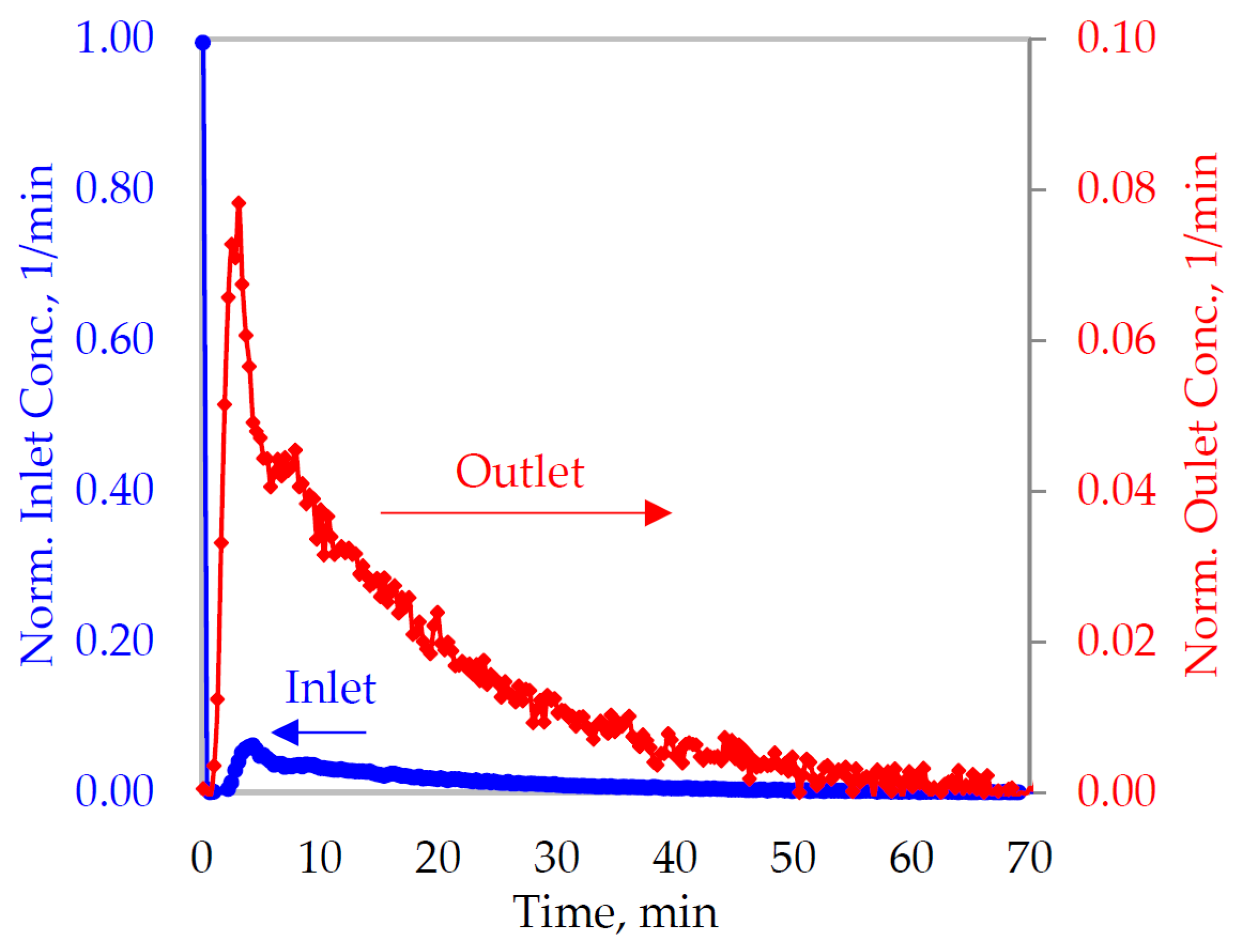Figure 2 illustrates inlet and outlet tracer concentrations in the ball mill BM1, showing the impact of the tracer recirculation on these measurements. The inlet signal (in blue) was then the superposition of the initial tracer injection (peak at t = 0) and a secondary signal from the hydrocyclone underflows (circulating load). The secondary signal also affected the outlet tracer concentration. It should be noted that the tracer injection was almost instantaneous with respect to the process dynamic and tracer recirculation. However, the outlet tracer signal in Figure 2 (in red) was not the mill RTD for this experimental condition. Deconvolution techniques were then required for the RTD estimation as the inlet signal significantly deviated from an impulse. The methodology presented here allows for the RTD estimations of the injected tracer. Therefore, a special attention must be paid when characterizing RTDs at specific particle sizes, as the traced component will also be observed in finer classes due to the grinding process.

3. RTD Estimation in Industrial Ball Mills

The outlet signal of a linear system y(t) is obtained by the convolution of the inlet signal x(t) and its impulse response h(t) as shown in Equation (1). Within Equation (1), the impulse response corresponds to the RTD.

$$y\left(t\right)={{\displaystyle \int }}_0^{\infty }x\left(t-\tau \right)h\left(\tau \right)d\tau =x\left(t\right)\times h\left(t\right)$$

(1)

For discretised inlet and outlet signals (x and y, respectively), Equation (1) can be expressed as a function of the convolution operator  [21]. This operator is defined by the inlet signal x.

$$y=\widehat{A} h$$

(2)

Thus, h can be obtained from the inversion of Equation (2). In the absence of noise in x and y, and an invertible  matrix, the estimation of h is numerically stable and guarantees unicity [21]. However, the inlet and outlet signals are subject to measurement noise, which typically hinders the h estimation. Under inlet signals with high auto-dependence, the  operator may be rank-deficient, rendering the inversion problem of Equation (2) ill-posed [21,22,23,24]. As the inlet signal is commonly subject to recirculation in grinding circuits, the h estimation from Equation (2) is not straightforward due to the x autocorrelation. This work compared two strategies to estimate h, which avoided the direct inversion of Equation (2): (i) a numerical linear regression approach subject to non-negativity in h (constrained least-squares estimation); and (ii) a parametric method that assumed a model structure for h, and whose parameters were obtained by non-linear regression.

3.1. Constrained Least-Squares Estimation

A constrained least-squares estimation was used to estimate the residence time distribution in the ball mills. This approach considered a non-negativity constraint to avoid infeasible solutions. Equation (3) presents the optimization problem:

$$\begin{array}{c}\underset{h}{\min }{\left(\widehat{A} h-y\right)}^{\mathrm{T}}\left(\widehat{A} h-y\right)\\ \mathrm{subject}\mathrm{to}\text{:}\\ h\ge 0\end{array}$$

(3)

Equation (3) was solved in Matlab using the interior-point-convex quadprog, which is currently implemented in the lsqlin function [25]. The convolution operator  was constructed by the function convmtx of Matlab, using the inlet data as an argument [26]. The non-parametric RTD estimations from Equation (3) did not involve any assumption on the distribution shape.

3.2. Parametric Estimation

The solution provided by the constrained least-squares estimation was compared to a parametric estimation. In the parametric approach, a model structure for the residence time distribution was assumed. The N-perfectly-mixed-tanks-in-series model of Equation (4) was employed, including a transport delay τ_D. This model structure was chosen due to its flexibility, low number of parameters and consistency with the experimental data. Equation (4) allowed the industrial ball mills to be characterized as multistage mixing systems, with each stage having the same residence time τ.

$$\begin{array}{c}h\left(t\right)=\frac{{\left(t-{\tau }_D\right)}^{\left(N-1\right)}\exp \left[-\frac{\left(t-{\tau }_D\right)}{\tau }\right]}{{\tau }^N\mathsf{\Gamma }\left(N\right)}\\ t\ge {\tau }_D\\ {\tau }_{\mathrm{mean}}=N\tau +{\tau }_D\end{array}$$

(4)

Within Equation (4), N corresponds to the number of mixers in series and Γ(N) to the Gamma function. This Gamma function extends the factorial function to non-integer arguments. For a discretization scheme for x, y and h, the model parameters were obtained by non-linear regression, according to Equation (5). This optimization problem was implemented in Matlab, using unconstrained minimization by the fminsearch function, which solves a quasi-Newton algorithm [27]. The convolution operator was again constructed as a function of the inlet data by the convmtx function of Matlab [26]. More details on the implementation of fminsearch can be found in [27].

$$\underset{\tau , {\tau }_D, N }{\min }{\left(\widehat{A} h-y\right)}^{\mathrm{T}}\left(\widehat{A} h-y\right)$$

(5)

From the solutions of Equations (3) and (5) for the proposed deconvolution approaches, the agreements between the RTD shapes, and the mean and median residence times are discussed.

Compared to all studies reported in literature and detailed in Table 1, the identification approach presented here has the following features:

• The concentrations are measured on-stream without process disturbances associated with sampling.
• No assumptions are made on the tracer injection, because the inlet concentration is directly measured in the industrial machines.
• Mass balances are not required to account for the tracer recirculation to the inlet stream.
• No assumptions are made on the mixing regimes in each circuit constituent.
• The inversion problem is numerically solved to avoid the bad conditioning of Equation (1) caused by the tracer recirculation in the ball mill-classifier circuits.

The integration of all these features for the estimation of ball mills RTDs (closed-circuit) at a large scale has not been reported to date. To identify these RTDs, the tracer activity must be adequately determined for the industrial tests, taking the activity decays and feed flowrates into consideration. Sufficiently high sampling rates are required in the measurement system to observe the process dynamics. Although the radioactive tracer technique allowed for high sampling rates, signal pre-processing was conducted to increase the signal-to-noise ratios, rejecting part of the measurement noise. This pre-processing stage was defined to filter all signals without losing information on the system responses. It should be noted that both adequate tracer activities and signal pre-processing are critical for an adequate RTD identification in closed-circuit ball mills, due to the high autocorrelation of the inlet concentrations, caused by the tracer recirculation.

4. Results

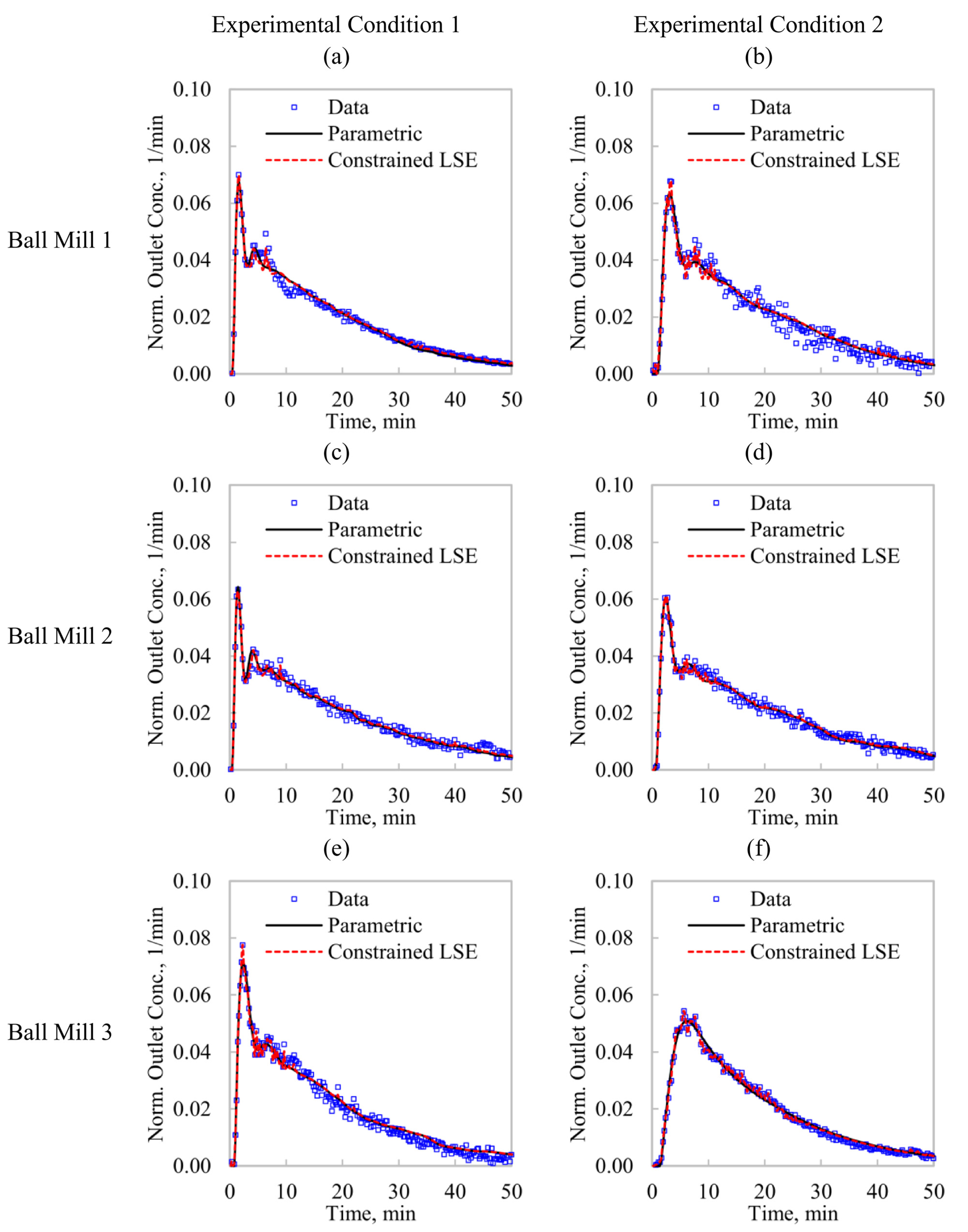
Figure 3 and Figure 4 compare the model fitting (output reconstruction) and RTD estimations, respectively, from the studied methodologies (Equations (3) and (5)). Two experimental conditions are presented for each ball mill. From Figure 3, an adequate model fitting is observed with both identification techniques. The constrained LSE allowed for more flexibility, leading to a higher sensitivity to measurement noise, which explains some variability in the outlet signal reconstruction. The parametric estimation showed a better rejection to the experimental variability, filtering the inlet tracer signals and smoothing the model fitting. Figure 3a–e, show the outlet signals as the superposition of the first pass of the tracer (first peak) throughout the mill and secondary signals caused by the circulating loads towards the mill feeds (hydrocyclone underflows). This effect is less clear in Figure 3f for the ball mill BM3 due to a longer mean residence time, which favored the dispersion of the first pass of the tracer. 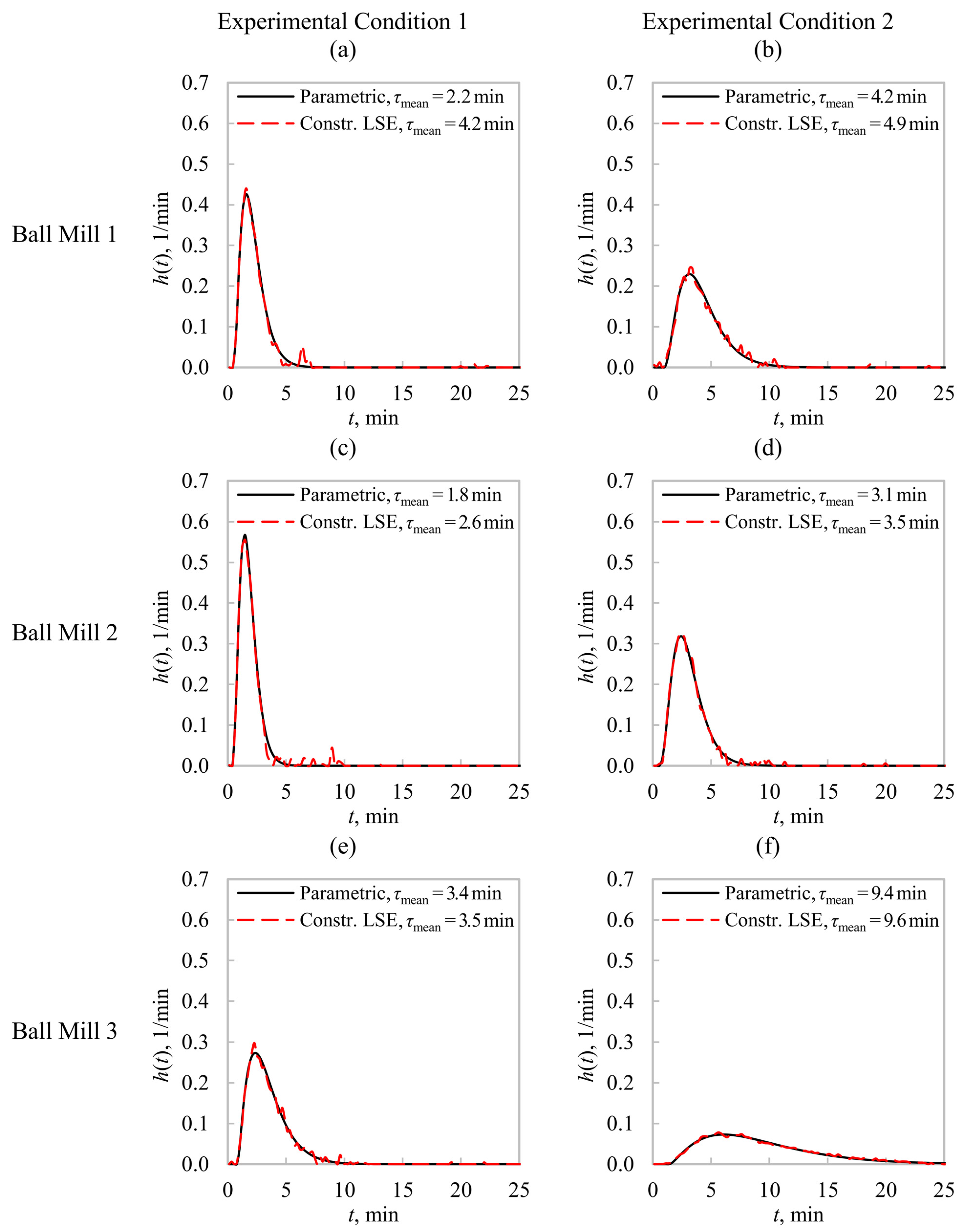Figure 4 shows a good agreement between the estimation methodologies for the RTDs (h(t)), with both approaches converging to residence time distributions with approximately the same shape. The constrained LSE led to h(t) distributions with higher variability, showing its sensitivity to the measurement noise. All distributions tended to mound-shaped distributions, which implies significant differences with respect to single perfect mixers (pure exponential h(t)s). In addition, these mounded h(t)s indicate regimes consisting of more than one perfect mixer (in series) due to the influence of the Central Limit Theorem. This result was forced in the parametric method by assuming that h(t) follows Equation (4); however, the constrained LSE approached the same h(t)s with no assumptions on the RTD shapes.

Table 2. Mean and median residence times obtained from the parametric deconvolution and the constrained LSE. The number of equivalent perfect mixers in series is also presented. Information sorted from the lowest to the highest τ₅₀ for the three replicates.

	Parametric Estimation			Constrained LSE
Mill	N	τmean, min	τ50, min	τmean, min	τ50, min
Ball Mill 1	2.7, 2.7, 3.1	2.2, 3.9, 4.2	2.0, 3.6, 3.8	4.2, 4.7, 4.9	2.1, 3.6, 3.9
Ball Mill 2	3.9, 2.2, 3.8	1.8, 2.5, 3.1	1.7, 2.2, 2.9	2.6, 4.6, 3.5	1.7, 2.3, 2.9
Ball Mill 3	2.4, 2.1, 2.4	3.4, 3.9, 9.4	3.1, 3.4, 8.3	3.5, 4.4, 9.6	3.1, 3.5, 8.3

summarizes the mean and median solid residence times. The number of equivalent perfect mixers in series is also presented for the parametric approach, which was greater than 2 in all cases. The median residence times τ₅₀ were consistent between the two studied estimation methodologies. However, the τ_mean values were in some cases significantly higher when estimated from the constrained LSE, due to the presence of rapid variations at long residence times. This condition is caused by the influence of noisy signals on the estimated h(t)s, which distorts τ_mean due to its sensitivity to extreme values. This limitation is common in numerical inversion methods derived from Equation (2). The lower median sensitivity to these extreme values justifies the τ₅₀ agreements shown in Table 2 between the studied methodologies.

The results in Figure 4 and Table 2 show the potential of the estimation methodologies, presented here, to characterize RTDs in industrial ball mills. The approaches did not require mass balances nor assumptions on the tracer recirculation and mixing in the constituents of the secondary grinding circuit, as reported in the literature and summarized in Table 1. Given an adequate model structure for h(t), the parametric estimates agreed with a direct inversion method such as the constrained LSE approach. Both strategies led to RTDs consistent with mound-shaped distributions, as previously reported in literature. 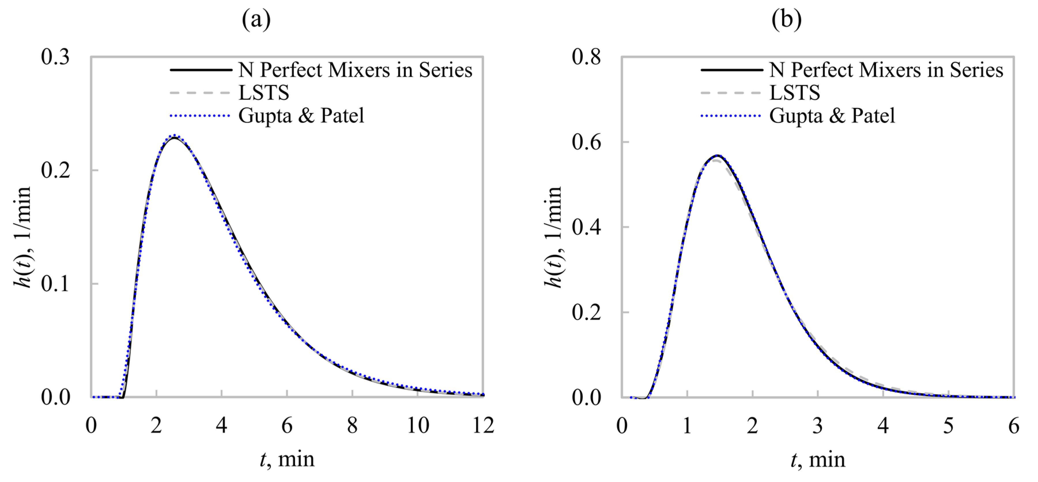Figure 5 illustrates ball mill RTDs obtained from the parametric method, using three model structures: (i) the N-perfectly-mixed-tanks-in-series model; (ii) the Large and Small Tanks in Series (LSTS) model [8]; and (iii) the geometric progression of perfect mixers in series reported by Gupta and Patel [7]. In all cases, transport delays were included to improve the model flexibility. Otherwise, poor model fitting was obtained. Negligible differences were obtained between these h(t) models because all of them showed sufficient flexibility to represent mounded RTDs. This result was caused by the representation of the RTDs as an in-series multistage system such that the experimental data were defined by the Central Limit Theorem. Therefore, no evidence of a more realistic model was observed from the studied data. Multistage RTDs with N ≈ 2–4 including a transport delay imply a moderate trend towards a plug flow regime, which favors the size reduction with respect to perfect mixing for the same residence time. The parametric deconvolution allowed for more consistent estimates for the mean residence times, taking the skewness of the RTDs into consideration. As shown in Figure 4, the RTD skewness approached zero (as h(t) approached mounded distributions), indicating similarities between τ_mean and τ₅₀. This feature was not observed with the constrained LSE due to its sensitivity to measurement noise that favored h(t) variations at long residence times. Thus, the parametric approach proved to be more suitable to characterize RTDs in closed-circuit ball mills at industrial scale. The constrained LSE method was also demonstrated to be a suitable tool to estimate the ball mill RTDs, with no assumption on the mixing regime. Although biases in the mean residence time can be observed, the RTD shapes can be detected from this estimate, which allows an adequate model structure for h(t) to be selected.

5. Conclusions

Residence time distribution measurements were conducted in balls mills, which were operated in closed-circuit with hydrocyclone racks. The radioactive tracer technique was used to measure the inlet and outlet solid concentrations in 3 industrial mills, in which the solid tracer corresponded to activated samples from the hydrocyclone underflow. Two methodologies were implemented to estimate the ball mill RTDs: (i) a non-parametric deconvolution based on a constrained least-squares algorithm; (ii) a parametric deconvolution, using the N-perfectly-mixed-tanks-in-series model to describe the RTDs. In both cases, the convolution of the inlet concentration with the estimated RTD allowed for the outlet signal reconstruction. From the RTD estimations and comparisons, the following results were obtained:

• The parametric and non-parametric estimations were consistent between each other, both leading to mound-shaped residence time distributions. This result implies significant differences with respect to perfect mixing.
• The number of perfectly mixed tanks in series ranged from 2 to 4, which indicated that the studied ball mill RTDs can be represented as a multi-stirring process. The RTD shapes were then a result of the Central Limit Theorem, approaching the mixing regime to a normal distribution.
• A comparison of the mean and median residence times from the studied deconvolution methodologies indicates that the non-parametric approach was sensitive to measurement noise, which led to inconsistencies between these two location indicators. As the parametric approach led to more consistent relationships between the mean and median residence times for RTDs converging to normal distributions, this methodology was more suitable to characterize closed-circuit ball mills.

The system identification techniques presented here proved to be applicable to industrial closed-circuit ball mills. These techniques did not require assumptions on the tracer recirculation and mixing in the sump boxes, pipelines and hydrocyclone racks.