
Audio Magnetotellurics Study of the Geoelectric Structure across the Zhugongtang Giant Lead–Zinc Deposit, NW Guizhou Province, China
 ,
,
Abstract
:1. Introduction
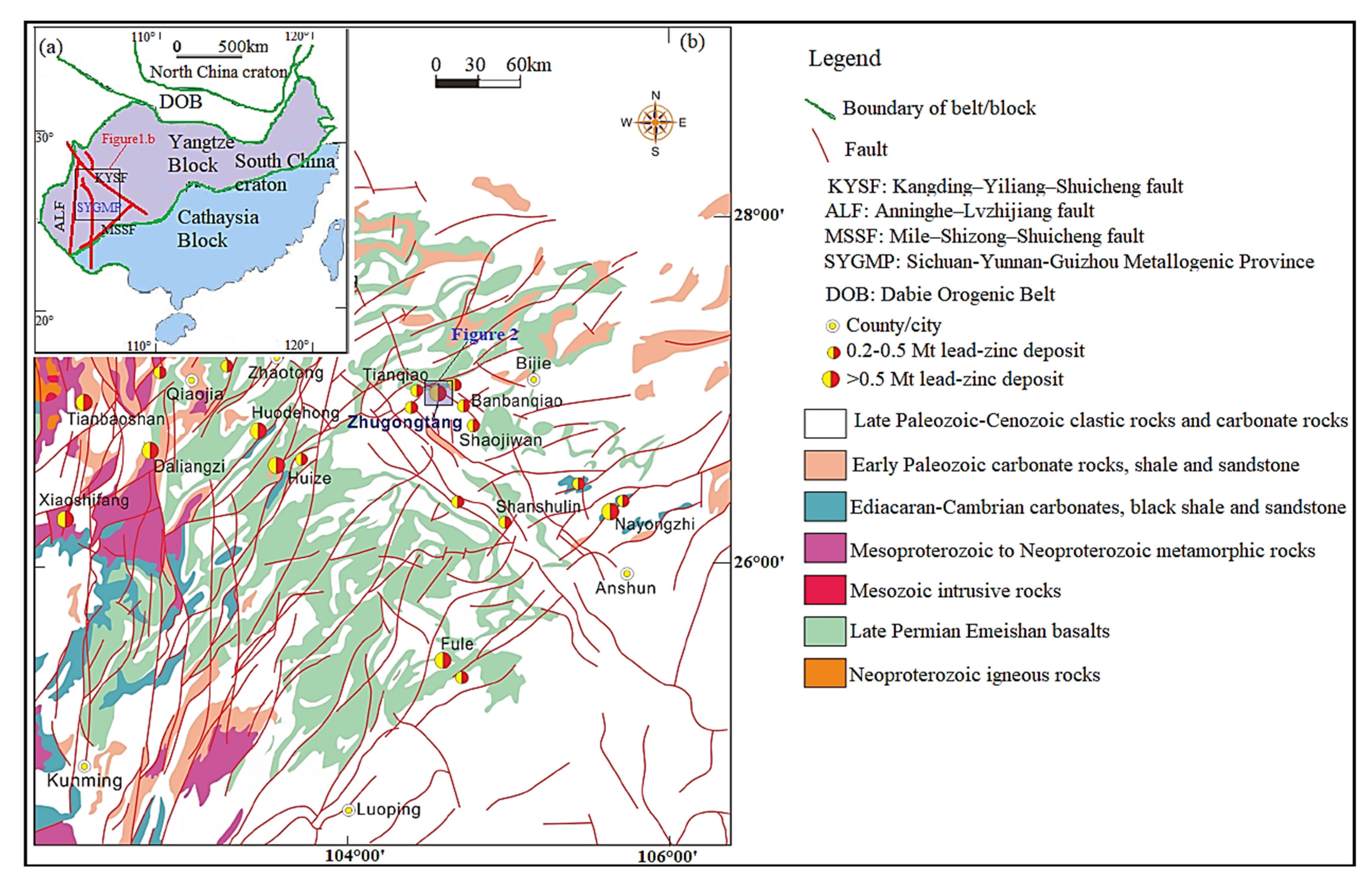
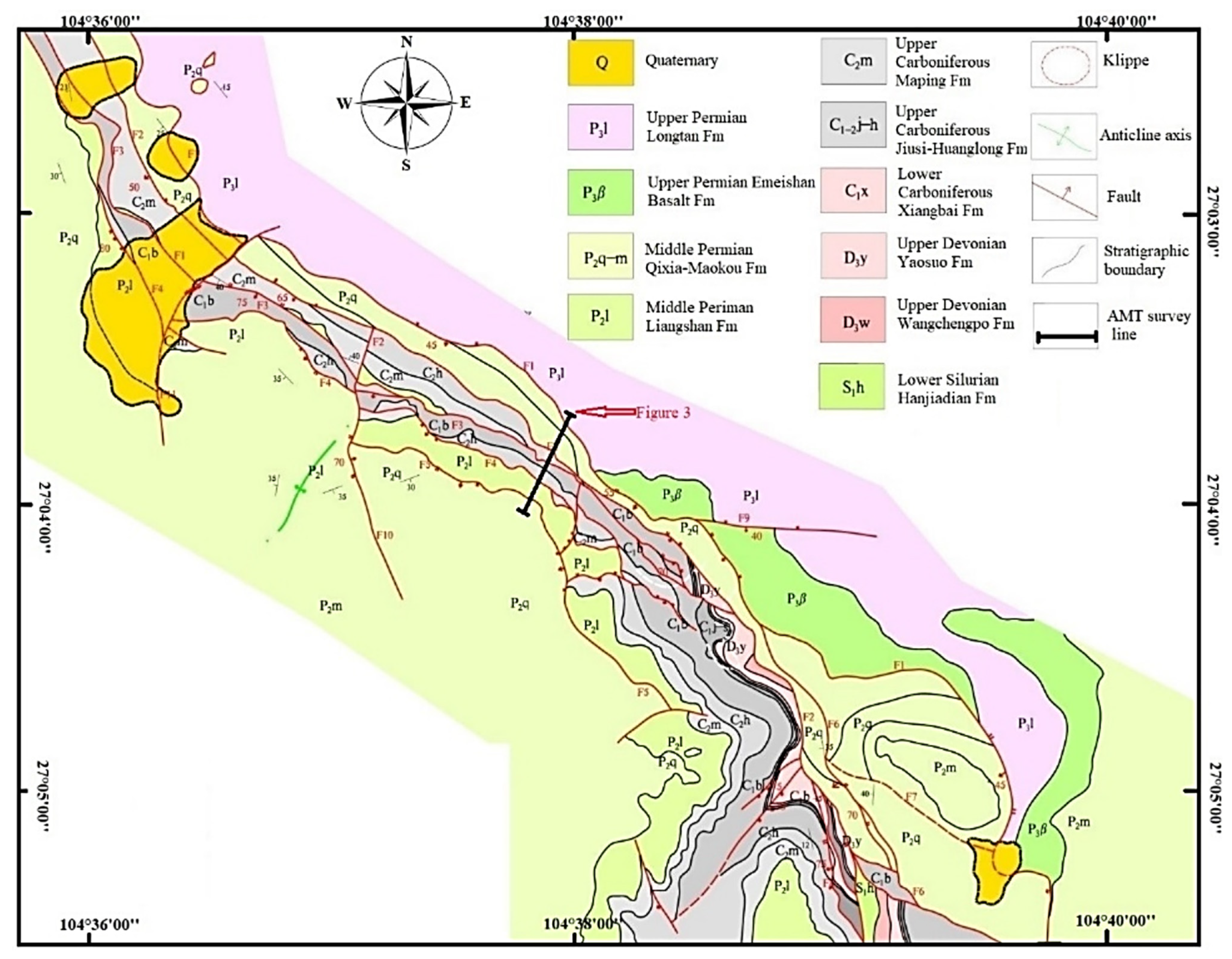
2. Geological Setting
3. Deposit Geology
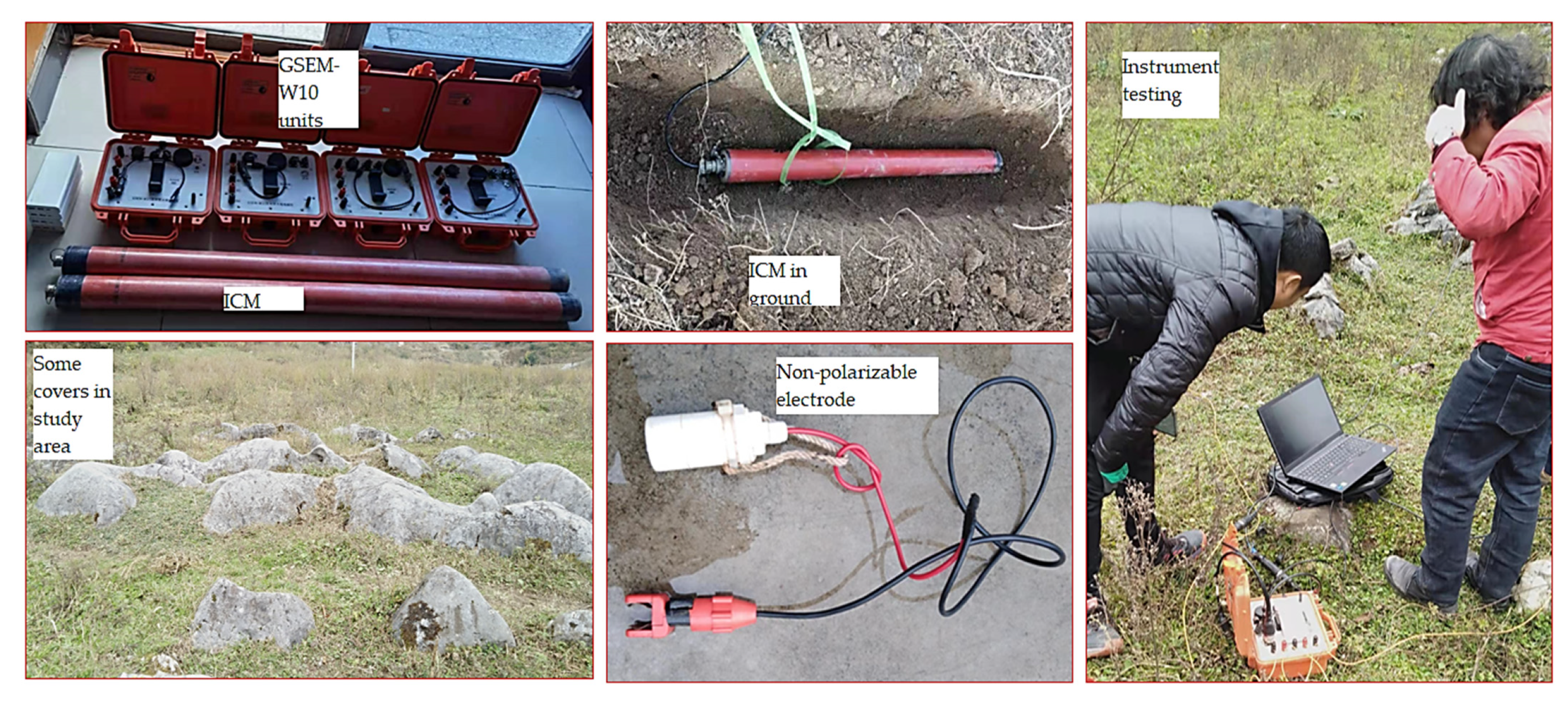
4. Methods
5. Data Acquisition and Processing
6. Data Analysis
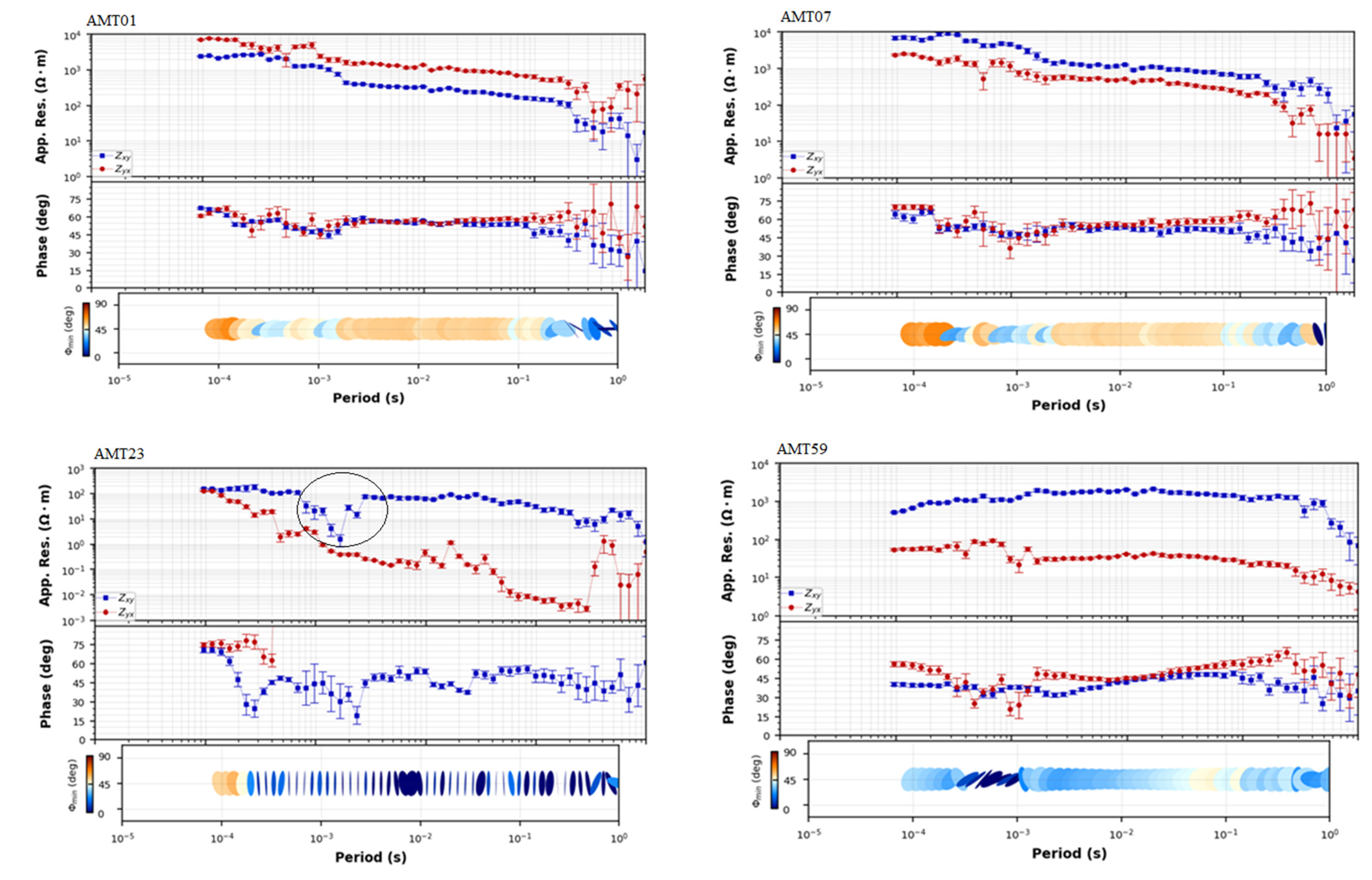
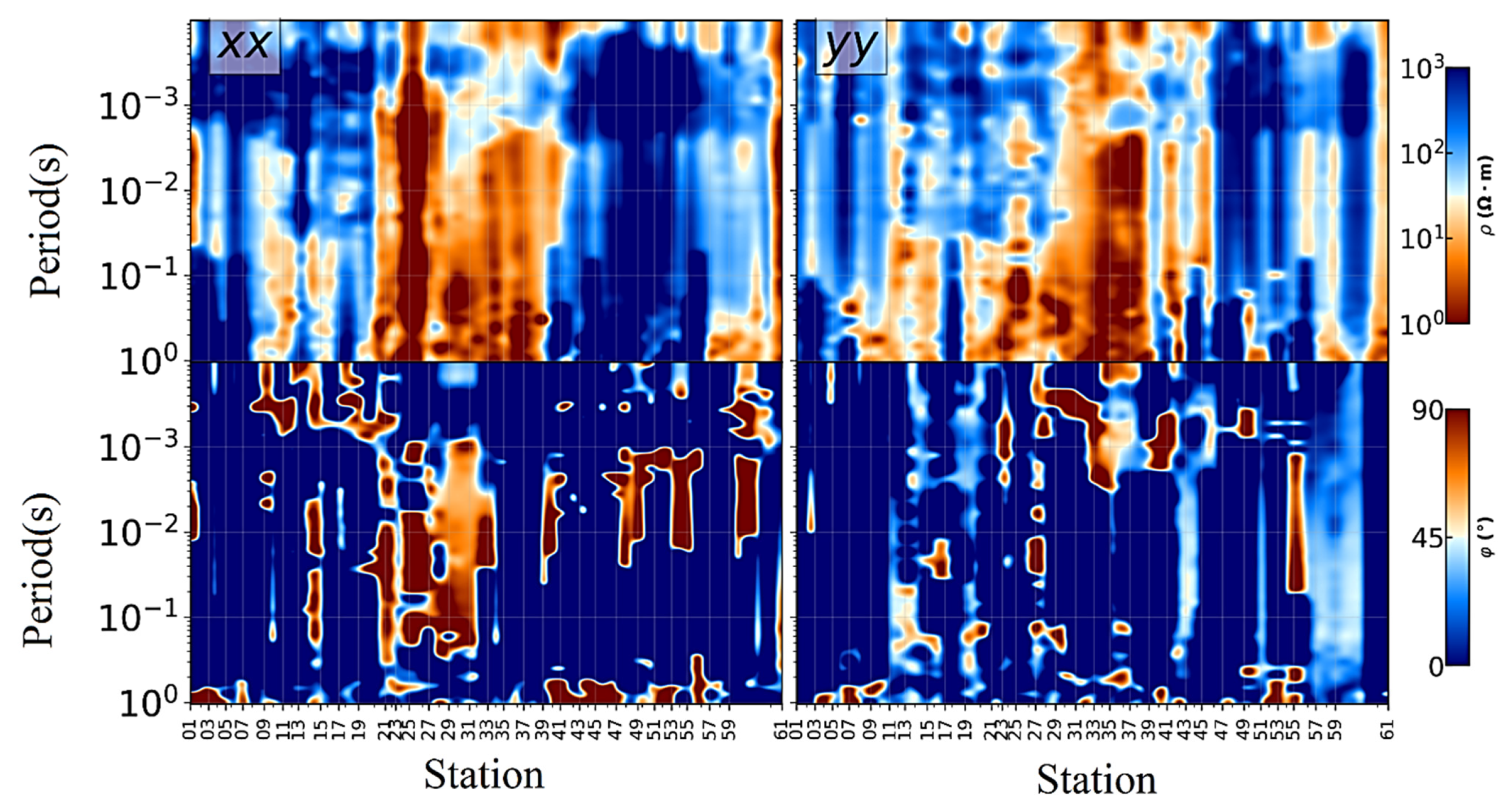
6.1. Apparent Resistivity-Phase Curves and Pseudo-Sections
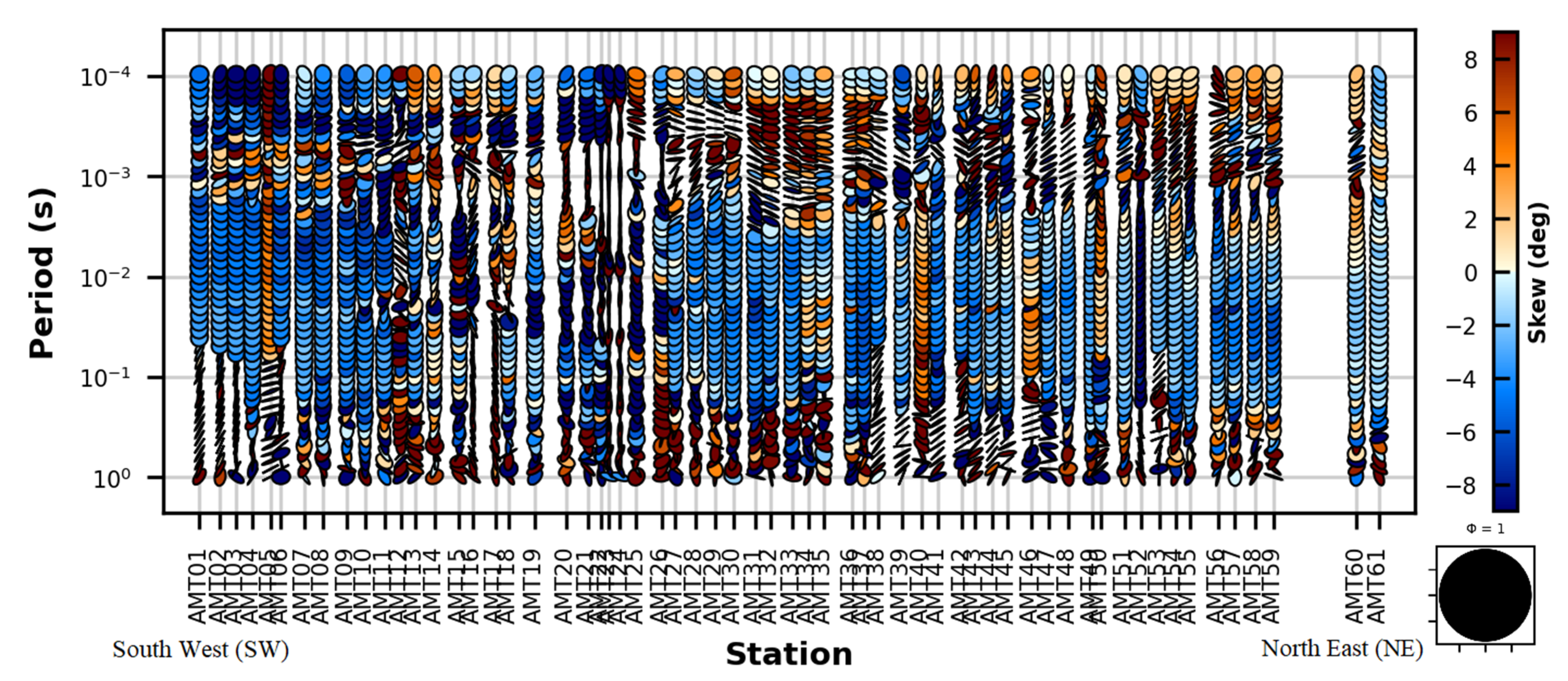
6.2. Dimensionality Analysis
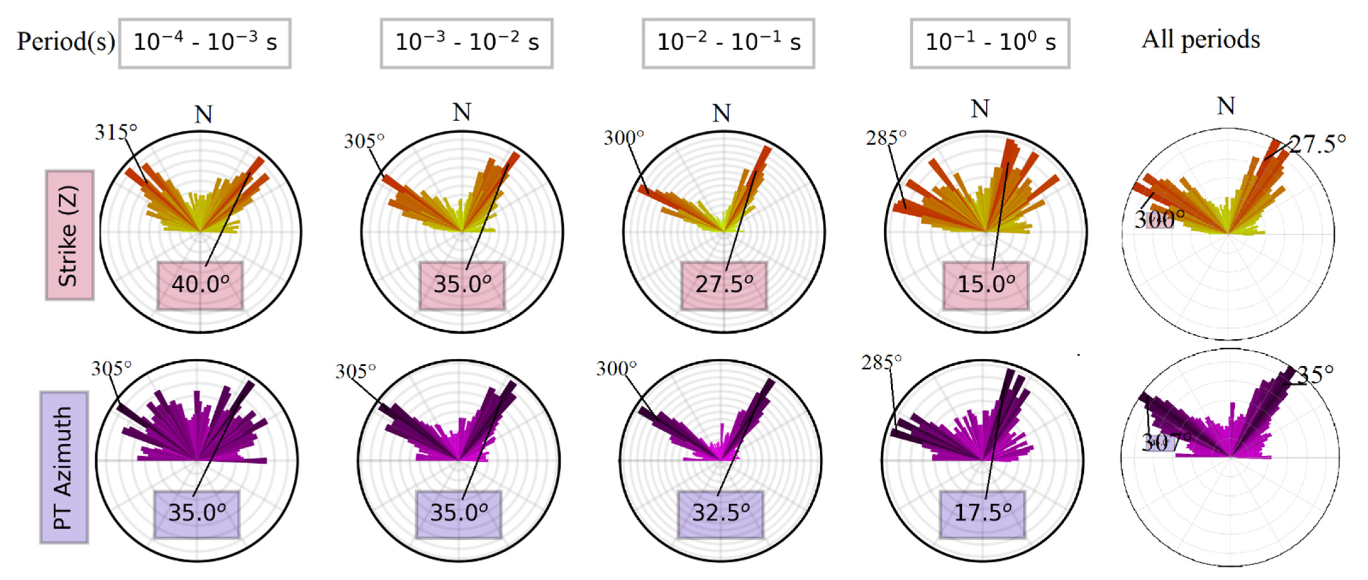
6.3. Geoelectric Strike Estimation
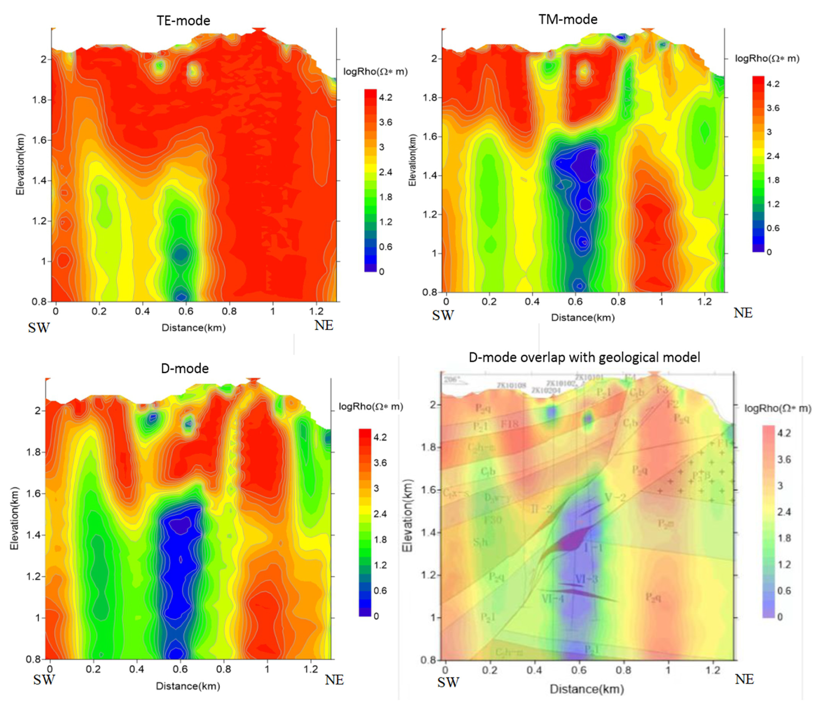
7. Two-Dimensional Inversion
8. Results and Discussion
9. Conclusions
Author Contributions
Funding
Data Availability Statement
Acknowledgments
Conflicts of Interest
References
- Andrieu, B.; Vidal, O.; le Boulzec, H.; Verzier, F. Modelling the Demand and Access of Mineral Resources in a Changing World. Sustainability 2022, 14, 11. [Google Scholar]
- Nkuna, R.; Ijoma, G.; Matambo, T.; Chimwani, N. Accessing Metals from Low-Grade Ores and the Environmental Impact Considerations: A Review of the Perspectives of Conventional versus Bioleaching Strategies. Minerals 2022, 12, 506. [Google Scholar] [CrossRef]
- Zhdanov, M.S. Editorial for Special Issue Geophysics for Mineral Exploration. Minerals 2021, 11, 692. [Google Scholar] [CrossRef]
- Zhang, G.; Lü, Q.T.; Zhang, G.B.; Lin, P.R.; Jia, Z.Y.; Suo, K. Joint interpretation of geological, magnetic, AMT, and ERT data for mineral exploration in the Northeast of Inner Mongolia, China. Pure Appl. Geophys. 2018, 175, 989–1002. [Google Scholar] [CrossRef]
- Zhao, P.; Cheng, Q.; Xia, Q. Quantitative Prediction for Deep Mineral Exploration. J. China Univ. Geosci. 2008, 19, 309–318. [Google Scholar]
- Fu, J.; Jia, S.; Wang, E. Combined Magnetic, Transient Electromagnetic, and Magnetotelluric Methods to Detect a BIF-Type Concealed Iron Ore Body: A Case Study in Gongchangling Iron Ore Concentration Area, Southern Liaoning Province, China. Minerals 2020, 10, 1044. [Google Scholar] [CrossRef]
- Embeng, S.B.N.; Meying, A.; Ndougsa-Mbarga, T.; Moreira, C.A.; Amougou, O.U.O. Delineation and Quasi-3D Modeling of Gold Mineralization Using Self-Potential (SP), Electrical Resistivity Tomography (ERT), and Induced Polarization (IP) Methods in Yassa Village, Adamawa, Cameroon: A Case Study. Pure Appl. Geophys. 2022, 179, 795–815. [Google Scholar] [CrossRef]
- Zhang, J.; Zeng, Z.; Zhao, X.; Li, J.; Zhou, Y.; Gong, M. Deep Mineral Exploration of the Jinchuan Cu–Ni Sulfide Deposit Based on Aeromagnetic, Gravity, and CSAMT Methods. Minerals 2020, 10, 168. [Google Scholar] [CrossRef] [Green Version]
- Jiang, W.; Duan, J.; Michael, D.; Clark, A.; Schofield, A.; Brodie, R.C.; Goodwin, J. Application of multiscale magnetotelluric data to mineral exploration: An example from the east Tennant region, Northern Australia. Geophys. J. Int. 2022, 229, 1628–1645. [Google Scholar] [CrossRef]
- Gan, J.; Li, H.; He, Z.; Gan, Y.; Mu, J.; Liu, H.; Wang, L. Application and Significance of Geological, Geochemical, and Geophysical Methods in the Nanpo Gold Field in Laos. Minerals 2022, 12, 96. [Google Scholar] [CrossRef]
- Lap, T.T. Application of Audio-Magnetotelluric Method for Exploration the Concealed Ore-Bodies in Yuele Lead-Zinc Ore Feild, Daguan County, NE Yunnan Province, China. J. Geosci. Environ. Prot. 2014, 2, 35–45. [Google Scholar] [CrossRef]
- Lap, T.T.; Xue, C.; Qureshijavedakhter; Wei, A.; Liu, L.; Li, W. Audio-Magnetotelluric Surveying and Its Application For The Concealed Orebodies Prospecting In Yuele Lead-Zinc Deposit Area, Daguan District, Northeastern Yunnan Province, China. Int. J. Appl. Nat. Sci. 2014, 3, 5–14. [Google Scholar]
- Chen, R.; He, M.; Chang, F.; Zeng, P.; Zhao, X. Large-scale 3-D inversion of AMT data with application to mineral exploration. In Proceedings of the 23rd Electromagnetic Induction Workshop—EMIW2016, Chiang Mai, Thailand, 14–21 August 2016. [Google Scholar]
- Bagchi, A.; Shalivahan, R.K.S.; Sinharay, R.K. 3D Phase tensor inversion and Joint inversion using impedance and phase tensor components aiming better subsurface mapping and interpretation in Dhanjori basin, Singhbhum craton, eastern India. J. Appl. Geophys. 2022, 202, 104646. [Google Scholar] [CrossRef]
- Bastani, M.; Malehmir, A.; Ismail, N.; Pedersen, L.B.; Hedjazi, F. Delineating hydrothermal stockwork copper deposits using controlled-source and radio-magnetotelluric methods: A case study from northeast Iran. Geophysics 2009, 74, B167–B181. [Google Scholar] [CrossRef]
- Agyemang, V.O. Groundwater exploration by magnetotelluric method within the birimian rocks of mankessim, Ghana. Appl. Water Sci. 2022, 12, 26. [Google Scholar] [CrossRef]
- Carlson, N.R.; Paski, P.M.; Urquhart, S.A. Applications of Controlled Source and Natural Source Audio-Frequency Magnetotellurics to Groundwater Exploration. In Proceedings of the 18th EEGS Symposium on the Application of Geophysics to Engineering and Environmental Problems, Atlanta, GA, USA, 3–7 April 2005. [Google Scholar]
- Zaher, M.A.; Younis, A.; Shaaban, H.; Mohamaden, M.I. Integration of geophysical methods for groundwater exploration: A case study of El Sheikh Marzouq area, Farafra Oasis, Egypt. Egypt. J. Aquat. Res. 2021, 47, 239–244. [Google Scholar] [CrossRef]
- He, G.L.; Wang, G.J.; Zhou, C.; Yan, X.L.; Li, H.L. Application of Audio-frequency Magnetotelluric (AMT) in groundwater exploration: A case of the Nanmushui area in Zhanjiang. Prog. Geophys. 2019, 34, 304–309. [Google Scholar]
- Ishizu, K.; Ogawa, Y.; Mogi, T.; Yamaya, Y.; Uchida, T. Ability of the magnetotelluric method to image a deep conductor: Exploration of a supercritical geothermal system. Geothermics 2021, 96, 102205. [Google Scholar] [CrossRef]
- He, L.; Chen, L.; Xi, X.; Zhao, X.; Chen, R.; Yao, H. Mapping the Geothermal System Using AMT and MT in the Mapamyum (QP) Field, Lake Manasarovar, Southwestern Tibet. Energies 2016, 9, 855. [Google Scholar] [CrossRef] [Green Version]
- Deshmukh, V.; Kumar, P.V.; Rao, P.S.; Kumar, A.; Singh, A. Audiomagnetotelluric (AMT) studies across Aravali-Tural-Rajawadi geothermal zones, western Maharastra, India. J. Appl. Geophys. 2022, 198, 104579. [Google Scholar] [CrossRef]
- Sandberg, S.K.; Hohmann, G.W. Controlled-source audiomagnetotellurics in geothermal exploration. Geophysics 1982, 47, 100–116. [Google Scholar] [CrossRef]
- Wu, G.; Hu, X.; Huo, G.; Zhou, X. Geophysical exploration for geothermal resources: An application of MT and CSAMT in Jiangxia, Wuhan, China. J. Earth Sci. 2012, 23, 757–767. [Google Scholar] [CrossRef]
- Min, G.; Wang, X.; Zhang, J.; Liu, K.; Yuan, H. The Concept of Multi-scale MT Interpretation Strategy and Its Application in Guizhou Province of China. Pure Appl. Geophys. 2022, 179, 1037–1051. [Google Scholar] [CrossRef]
- Robertson, K.; Taylor, D.; Thiel, S.; Heinson, G. Magnetotelluric evidence for serpentinisation in a Cambrian subduction zone beneath the Delamerian Orogen, southeast Australia. Gondwana Res. 2015, 28, 601–611. [Google Scholar] [CrossRef]
- Share, P.E.; Jones, A.G.; Muller, M.R.; Khoza, D.T.; Miensopust, M.P.; Webb, S.J. An audio-magnetotelluric investigation of the Otjiwarongo and Katima Mulilo regions, Namibia. Geophysics 2014, 79, B151–B171. [Google Scholar] [CrossRef] [Green Version]
- Bastani, M.; Wang, S.; Malehmir, A.; Mehta, S. Radio-magnetotelluric and controlled-source magnetotelluric surveys on a frozen lake: Opportunities for urban applications in Nordic countries. Near Surf. Geophys. 2022, 20, 30–45. [Google Scholar] [CrossRef]
- Mehta, S. Radio Magnetotelluric (RMT) measurement over lake Mälaren, Sweden: A case study. Geol. Geophys. Environ. 2015, 41, 110. [Google Scholar] [CrossRef]
- Mehta, S.; Bastani, M.; Malehmir, A.; Pedersen, L.B. Resolution and sensitivity of boat-towed RMT data to delineate fracture zones–example of the Stockholm bypass multi-lane tunnel. J. Appl. Geophys. 2017, 139, 131–143. [Google Scholar] [CrossRef]
- Saraev, A.; Antashuk, K.; Simakov, A.; Shlykov, A.; Konkov, A. Near surface exploration for horizontal welling using CSRMT method: Case study. In Proceedings of the International Conference on Engineering Geophysics, Al Ain, United Arab Emirates, 9–12 October 2017. [Google Scholar]
- Tezkan, B.; Hördt, A.; Gobashy, M. Two-dimensional radiomagnetotelluric investigation of industrial and domestic waste sites in Germany. J. Appl. Geophys. 2000, 44, 237–256. [Google Scholar] [CrossRef]
- Wang, S.; Malehmir, A.; Bastani, M. Geophysical characterization of areas prone to quick-clay landslides using radio-magnetotelluric and seismic methods. Tectonophysics 2016, 677–678, 248–260. [Google Scholar] [CrossRef]
- Luo, K.; Zhou, J.X.; Sun, G.T.; Nguyen, A.; Qin, Z.X. The metallogeny of the Devonian sediment-hosted sulfide deposits, South China: A case study of the Huodehong deposit. Ore Geol. Rev. 2022, 143, 104747. [Google Scholar] [CrossRef]
- Wei, C.; Huang, Z.; Ye, L.; Hu, Y.; Santosh, M.; Wu, T.; He, L.; Zhang, J.; He, Z.; Xiang, Z.; et al. Genesis of carbonate-hosted Zn-Pb deposits in the Late Indosinian thrust and fold systems: An example of the newly discovered giant Zhugongtang deposit, South China. J. Asian Earth Sci. 2021, 220, 104914. [Google Scholar] [CrossRef]
- Metcalfe, I. Palaeozoic and Mesozoic tectonic evolution and palaeogeography of East Asian crustal fragments: The Korean Peninsula in context. Gondwana Res. 2006, 9, 24–46. [Google Scholar] [CrossRef]
- Charvet, J.; Shu, L.; Shi, Y.; Guo, L.; Faure, M. The building of south China: Collision of Yangzi and Cathaysia blocks, problems and tentative answers. J. Southeast Asian Earth Sci. 1996, 13, 223–235. [Google Scholar] [CrossRef]
- Zhang, W.D.; You, H.T.; Li, B.; Zhao, K.D.; Chen, X.D.; Zhu, L. Ore-forming processes of the Qixiashan carbonate-hosted Pb-Zn deposit, South China: Constraints from sulfide trace elements and sulfur isotopes. Ore Geol. Rev. 2022, 143, 104786. [Google Scholar] [CrossRef]
- Zhang, C.; Wu, Y.; Hou, L.; Mao, J. Geodynamic setting of mineralization of Mississippi Valley-type deposits in world-class Sichuan–Yunnan–Guizhou Zn–Pb triangle, southwest China: Implications from age-dating studies in the past decade and the Sm–Nd age of Jinshachang deposit. J. Asian Earth Sci. 2015, 103, 103–114. [Google Scholar] [CrossRef]
- Yang, Q.; Liu, W.; Zhang, J.; Wang, J.; Zhang, X. Formation of Pb–Zn deposits in the Sichuan–Yunnan–Guizhou triangle linked to the Youjiang foreland basin: Evidence from Rb–Sr age and in situ sulfur isotope analysis of the Maoping Pb–Zn deposit in northeastern Yunnan Province, southeast China. Ore Geol. Rev. 2019, 107, 780–800. [Google Scholar] [CrossRef]
- Oyebamiji, A.; Hu, R.; Zhao, C.; Zafar, T. Origin of the Triassic Qilinchang Pb-Zn deposit in the western Yangtze block, SW China: Insights from in-situ trace elemental compositions of base metal sulphides. J. Asian Earth Sci. 2020, 192, 104292. [Google Scholar] [CrossRef]
- Wu, Y.; Zhang, C.; Mao, J.; Ouyang, H.; Sun, J. The genetic relationship between hydrocarbon systems and Mississippi Valley-type Zn–Pb deposits along the SW margin of Sichuan Basin, China. Int. Geol. Rev. 2013, 55, 941–957. [Google Scholar] [CrossRef]
- Zhao, D.; Han, R.; Wang, L.; Ren, T.; Wang, J.; Zhang, X.; Cui, J.; Ding, J. Genesis of the Lehong large zinc–lead deposit in northeastern Yunnan, China: Evidences from geological characteristics and C–H–O–S–Pb isotopic compositions. Ore Geol. Rev. 2021, 135, 104219. [Google Scholar] [CrossRef]
- Shen, X.; Lin, H.; Zhang, B.; Du, Q. The genesis of Guanting Pb–Zn deposits in the Jianshui area, Yunnan Province, SW China: Constraints from geochronology, S isotopes and trace elements. Mineral. Petrol. 2022, 116, 47–69. [Google Scholar] [CrossRef]
- Li, Z.X.; Li, X.H.; Wartho, J.A.; Clark, C.; Li, W.X.; Zhang, C.L.; Bao, C. Magmatic and metamorphic events during the early Paleozoic Wuyi Yunkai orogeny, southeastern South China: New age constraints and pressure-temperature conditions. GSA Bull. 2010, 122, 772–793. [Google Scholar] [CrossRef]
- Carter, A.; Clift, P.D. Was the Indosinian orogeny a Triassic mountain building or a thermotectonic reactivation event? Comptes Rendus Geosci. 2008, 340, 83–93. [Google Scholar] [CrossRef]
- Shellnutt, J.G.; Vaughan, M.W.; Lee, H.Y.; Iizuka, Y. Late Jurassic Leucogranites of Macau (SE China): A Record of Crustal Recycling During the Early Yanshanian Orogeny. Front. Earth Sci. 2020, 8, 311. [Google Scholar] [CrossRef]
- Zhou, J.X.; Xiang, Z.Z.; Zhou, M.F.; Feng, Y.X.; Luo, K.; Huang, Z.L.; Wu, T. The giant Upper Yangtze Pb–Zn province in SW China: Reviews, new advances and a new genetic model. J. Asian Earth Sci. 2018, 154, 280–315. [Google Scholar] [CrossRef] [Green Version]
- He, L.; Wu, D.; Zhao, F.; Jin, X.; Bai, G.; Chen, Z.; Wang, J.; Huang, Q.; Cai, J. Geological Characteristics, Exploration Model and Prospecting Direction of the Zhugongtang Ultra—large Pb—Zn deposit in Guizhou Province. Guizhou Geol. 2019, 36, 101–109, (In Chinese with English Abstract). [Google Scholar]
- Tikhonov, A.N. On determining electrical characteristics of the deep layers of the Earth’s crust. Doklady 1950, 73, 281–285. [Google Scholar]
- Cagniard, L. Basic theory of the magneto-telluric method of geophysical prospecting. Geophysics 1953, 18, 605–635. [Google Scholar] [CrossRef]
- Cantwell, T. Detection and Analysis of Low Frequency Magnetotelluric Signals. Doctoral Dissertation, Massachusetts Institute of Technology, Cambridge, MA, USA, 1960. [Google Scholar]
- Cantwell, T.; Madden, T.R. Preliminary report on crustal magnetotelluric measurements. J. Geophys. Res. 1960, 65, 4202–4205. [Google Scholar] [CrossRef]
- Vozoff, K. The magnetotelluric method in the exploration of sedimentary basins. Geophysics 1972, 37, 98–141. [Google Scholar] [CrossRef]
- Singh, R.K.; Shalivahan, V.P.M.; Singh, S. Imaging Regional Geology and Au—Sulphide mineralization over Dhanjori greenstone belt: Implications from 3-D Inversion of Audio Magnetotelluric data and Petrophysical Characterization. Ore Geol. Rev. 2019, 106, 369–386. [Google Scholar] [CrossRef]
- Tezkan, B. Radiomagnetotellurics. In Groundwater Geophysics; Springer: Berlin/Heidelberg, Germany, 2009. [Google Scholar]
- Kalscheuer, T.; Juhojuntti, N.; Vaittinen, K. Two-Dimensional Magnetotelluric Modelling of Ore Deposits: Improvements in Model Constraints by Inclusion of Borehole Measurements. Surv. Geophys. 2018, 39, 467–507. [Google Scholar] [CrossRef] [Green Version]
- Chave, A.D.; Jones, A.G. The Magnetotelluric Method: Theory and Practice; Cambridge University Press: New York, NY, USA, 2012. [Google Scholar]
- Nabighian, M.N. Electromagnetic Methods in Apllied Geophysics 2; Nabighian, M.N., Ed.; Society of Exploration Geophysicists: Houston, TX, USA, 1991; pp. 641–712. [Google Scholar]
- Lindsay, M.D.; Spratt, J.; Occhipinti, S.A.; Aitken, A.R.; Dentith, M.C.; Hollis, J.A.; Tyler, I.M. Identifying mineral prospectivity using 3D magnetotelluric, potential field and geological data in the east Kimberley, Australia. Geol. Soc. Lond. Spec. Publ. 2017, 453, 247–268. [Google Scholar] [CrossRef]
- Li, F.; Zeng, Q.; Zhu, R.; Chu, S.; Xie, W.; Zhang, B.; Zhang, X. Application of the AMT Method to Gold Deposits: A Case Study in the Qinling Metallogenic Belt of North China Craton. Minerals 2021, 11, 1200. [Google Scholar] [CrossRef]
- GSAI Geophysics. Internet of Things Broadband Magnetotelluric Instrument GSEM-W10. GSAI Geophysics, [Online]. Available online: http://www.gs-ait.com/productinfo/432117.html (accessed on 10 October 2022).
- GSAI Geophysics. Electromagnetic Data Processing Software GSEM-Pros. GSAI Geophysics, [Online]. Available online: http://www.gs-ait.com/productinfo/432127.html (accessed on 10 October 2022).
- Kirkby, A.L.; Zhang, F.; Peacock, J.; Hassan, R.; Duan, J. The MTPy software package for magnetotelluric data analysis and visualisation. J. Open Source Softw. 2019, 4, 1358. [Google Scholar] [CrossRef]
- Krieger, L.; Peacock, J. MTpy: A Python toolbox for magnetotellurics. Comput. Geosci. 2014, 72, 167–175. [Google Scholar] [CrossRef]
- Caldwell, T.G.; Bibby, H.M.; Brown, C. The magnetotelluric phase tensor. Geophys. J. Int. 2004, 158, 457–469. [Google Scholar] [CrossRef] [Green Version]
- Booker, J.R. The magnetotelluric phase tensor: A critical review. Surv. Geophys. 2014, 35, 7–40. [Google Scholar] [CrossRef]
- Thiel, S.; Heinson, G.; Gray, D.R.; Gregory, R.T. Ophiolite emplacement in NE Oman: Constraints from magnetotelluric sounding. Geophys. J. Int. 2009, 176, 753–766. [Google Scholar] [CrossRef] [Green Version]
- Farzamian, M.; Ribeiro, J.A.; Khalil, M.A.; Santos, F.A.M.; Kashkouli, M.F.; Bortolozo, C.; Mendonça, J.L. Application of transient electromagnetic and audio-magnetotelluric methods for imaging the Monte real aquifer in Portugal. Pure Appl. Geophys. 2019, 176, 719–735. [Google Scholar] [CrossRef]
- Seki, K.; Kanda, W.; Ogawa, Y.; Tanbo, T.; Kobayashi, T.; Hino, Y.; Hase, H. Imaging the hydrothermal system beneath the Jigokudani valley, Tateyama volcano, Japan: Implications for structures controlling repeated phreatic eruptions from an audio-frequency magnetotelluric survey. Earth Planets Space 2015, 67, 6. [Google Scholar] [CrossRef] [Green Version]
- Niasari, S.W. A short introduction to geological strike and geo-electrical strike. AIP Conf. Proc. 2016, 1755, 100002. [Google Scholar]
- Wu, D.; He, L.; Cai, J.; Wang, J.; Bai, G.; Yang, T.; Jin, X.; Huang, Q. Main Orebody Characteristics and Ore—prospecting Symbols of Zhugongtang Lead—zinc Deposit in Hezhang, Guizhou. Guizhou Geol. 2019, 36, 299–306, (In Chinese with English Abstract). [Google Scholar]
- Weaver, J.T.; Agarwal, A.K.; Lilley, F.E.M. Characterization of the magnetotelluric tensor in terms of its invariants. Geophys. J. Int. 2000, 141, 321–336. [Google Scholar] [CrossRef] [Green Version]
- ZOND Geophysical Software, ZondMT2D. ZOND Geophysical Software, 2001–2022. Available online: http://zond-geo.com/english/zond-software/electromagnetic-sounding/zondmt2d/ (accessed on 20 March 2022).
- Unsworth, M.; Egbert, G.; Booker, J. High-resolution electromagnetic imaging of the San Andreas fault in Central California. J. Geophys. Res. 1999, 104, 1131–1150. [Google Scholar] [CrossRef]
- Maulinadya, S.; Grandis, H. Geoelectric Strike Analysis from Magnetotelluric (MT) Data Using Swift and Polar Diagram Methods. IOP Conf. Ser. Earth Environ. Sci. 2019, 318, 012049. [Google Scholar] [CrossRef] [Green Version]
- Berdichevsky, M.N.; Dmitriev, V.I.; Pozdnjakova, E.E. On two-dimensional interpretation of magnetotelluric soundings. Geophys. J. Int. 1998, 133, 585–606. [Google Scholar] [CrossRef]


| Rock and Ore Specimens | Average Resistively/Ωm | Present Study: AMT Resistivity Range/Ωm | |
|---|---|---|---|
| Dolomite and limestone | 5551–157,130 | ≥1000 | |
| Basalts | tuffaceous basalt | 517.3 | >63 (flood basalts) |
| massive basalt | 2384 | ||
| Shale, sandstone, claystone Silty mudstone | <100 | 4–63 | |
| Bioclastic limestone, dolomite limestone | >250 | ||
| Conductor (Pb-Zn) | 69.4 | <15 | |
Publisher’s Note: MDPI stays neutral with regard to jurisdictional claims in published maps and institutional affiliations. |
© 2022 by the authors. Licensee MDPI, Basel, Switzerland. This article is an open access article distributed under the terms and conditions of the Creative Commons Attribution (CC BY) license (https://creativecommons.org/licenses/by/4.0/).
Share and Cite
Pitiya, R.; Lu, M.; Chen, R.; Nong, G.; Chen, S.; Yao, H.; Shen, R.; Jiang, E. Audio Magnetotellurics Study of the Geoelectric Structure across the Zhugongtang Giant Lead–Zinc Deposit, NW Guizhou Province, China. Minerals 2022, 12, 1552. https://doi.org/10.3390/min12121552
Pitiya R, Lu M, Chen R, Nong G, Chen S, Yao H, Shen R, Jiang E. Audio Magnetotellurics Study of the Geoelectric Structure across the Zhugongtang Giant Lead–Zinc Deposit, NW Guizhou Province, China. Minerals. 2022; 12(12):1552. https://doi.org/10.3390/min12121552
Chicago/Turabian StylePitiya, Regean, Mao Lu, Rujun Chen, Guanhai Nong, Siwen Chen, Hongchun Yao, Ruijie Shen, and Enhua Jiang. 2022. "Audio Magnetotellurics Study of the Geoelectric Structure across the Zhugongtang Giant Lead–Zinc Deposit, NW Guizhou Province, China" Minerals 12, no. 12: 1552. https://doi.org/10.3390/min12121552