Image Segmentation Method on Quartz Particle-Size Detection by Deep Learning Networks

Abstract

In the beneficiation of quartz sand, hydraulic classification is a primary way to obtain quartz production in various size fractions. It is essential for plants to measure the particle size of quartz sand during the classification, in time to evaluate the classification efficiency. However, the traditional manual-screening method consumes labor and time, while the particle-size analyzer is expensive. Thus, a size-detection method of quartz-sand particle is proposed in this paper, which is based on a deep learning semantic-segmentation network Fully Convolutional Networks (FCN)-ResNet50. The FCN-ResNet50 network sand segments images, and the average particle size of quartz sand is obtained after converting the pixel-particle size to physical-particle size. Using deep learning, the quartz sand with particle sizes of −40 + 70 (0.212–0.38 mm), −70 + 100 (0.15–0.212 mm), −100 + 140 (0.109–0.15 mm), and −140 + 400 (0.038–0.109 mm) meshes, can be measured directly. The results showed that the validation accuracy of the FCN-ResNet50 was over 97%, and the loss value was approximately 0.2. Compared with the UNet-Mobile and Deeplab-Xception, the average error of particle-size detection was approximately 0.01 mm, which was close to the manual calibration-software results. This method has the advantages of quick sampling and low equipment costs, increasing the hydraulic-classification efficiency of quartz sand and promoting automation in the concentrator.

1. Introduction

1.1. Background

Quartz sand, also known as silica sand, is a silicate mineral with rigidity, wear resistance and stable chemical properties. As a vital industrial mineral-raw-material, quartz sand is applied within various industries, such as glass [1], ceramics [2], metallurgy [3], construction [4], and mechanical casting [5]. In the glass industry, quartz sand can be the primary raw material for quartz glass products and glass fiber. In the ceramic industry, quartz sand can be used as ceramic and refractory-ceramic embryo-material, and in the metallurgical industry, quartz sand can be used as silicon metal, silicon aluminum alloy, and other raw materials or additives and flux. In the construction industry, quartz sand can be used in concrete, road-building materials, and cement physical-property test materials, and in the mechanical casting industry quartz sand can be used to make power station castings, heavy-machinery castings, aviation castings and other high-end casting molds.

The particle-size distribution of quartz sand is significant for process application. Quartz sand with different particle sizes has different plasticity, mud viscosity, molding properties, drying and sintering performances. Commonly, quartz fractions of −40 + 70 mesh, −70 + 100 mesh, −100 + 140 mesh, and −140 + 400 mesh are often used in mineral processing and other industries. For example, quartz production of −40 + 70 mesh can be used as filling material for advanced vessel-glass, sandblasting, filter sand and sulfuric acid tower, while −70 + 100 mesh can be used for water filtration, ceramics and enamels. Therefore, the classification of quartz ore is of great importance for the industry.

Meanwhile, it is necessary to measure the size features of classification products. The manual screen method takes 30 min to obtain the size distribution of quartz, which is not efficient for quartz production in China. For most factories, the commonly used classification equipment, such as vibrating screen and hydraulic cyclone [6,7], are often used to measure coarse and fine particles, respectively, in classification. Other techniques such as laser diffraction and automated image analysis are also used to perform size measurements [8,9]. Laser diffraction enables fast and reliable online size measurement, but the online particle-size analyzer is too expensive for many factories. The automated image analysis can use the characteristic value of the two-dimensional image under the microscope to obtain the particle-size distribution, but the analysis error for fine particles is large.

Aimed at reducing cost and measurement time, and improving the detection accuracy of the quartz particle size, this study uses the deep learning method to perform image segmentation, so that the online analysis of sand particle size can be realized. If the particle size changes significantly, parameters of the classification equipment can be timely adjusted, then sampled and evaluated again until the granularity detection meets the requirements. The particle-size detection system saves costs and can quickly screen quartz sand with different particle sizes.

In the study of mineral segmentation, some scholars have proposed the mineral feature-extraction method of rock images based on multi-scale segmentation [10]. Some scholars have proposed the mineral segmentation method of ore microscopes based on color normalization statistics [11]. Recently, with the progress of artificial intelligence, the ultra-high prediction accuracy of deep learning segmentation-networks in computer vision has aroused considerable concern in ore dressing. Some scholars have proposed the use of deep learning networks such as U-Net and DeepLabv³⁺ for the semantic segmentation of ore particles [12,13,14]. Some scholars have proposed the use of a lightweight deep learning network for ore image segmentation [15,16]. Some scholars have also proposed the use of deep learning networks such as SegNet to segment bituminous coal maceral groups [17]. Deep learning segmentation networks can be applied well to mineral segmentation tasks. However, deep learning technology has not been fully exploited and applied within quartz-sand particle-size detection.

This work uses the deep learning semantic-segmentation network, Fully Convolutional Networks (FCN)-ResNet50 [18,19], and compares the two segmentation networks, UNet-Mobile [20,21] and Deeplab-Xception [22,23], to detect the quartz-sand granularity. Quartz sand particles are sampled in the hydraulic classification of the quartz-sand beneficiation industrial-process, and the sand image dataset is fed into the model for training to obtain the segmented prediction map with black and white labels. The area ratio of sand to background is obtained, and the average granularity of the sampled quartz sand with different meshes is calculated. Objects selected in this experiment are quartz-sand samples with different particle sizes of −40 + 70, −70 + 100, −100 + 140, and −140 + 400 meshes. Our particle-size detection system can quickly determine the particle size, improving the efficiency of quartz-sand beneficiation and purification.

1.2. Technology

Deep learning technology, with its super-high recognition accuracy, is widely used in biomedical and environmental science, industrial production, and other fields [24,25,26]. Deep neural networks, such as convolutional neural networks (CNNs), enable computers to automatically learn object features from numerous data, and can gradually replace traditional image-processing work based on algorithm description. CNNs can perform forward learning and reverse error-propagation. Feature learning and hierarchical feature extraction are efficient algorithms to replace manual feature extraction. CNNs comprise input, hidden, and output layers. The hidden layer could include convolutional, pooling, and fully connected layers. The traditional CNN connects several fully connected layers after the last convolution layer, and maps the feature map generated by the convolution layer to a feature vector with a fixed length for image-level classification and the regression task. The convolved feature-map size is represented by Equation (1) where W is the size of an input image, F is the kernel size, S is the stride, and Pad is the size of padding.

$$S_{output}=\frac{\left(W+2\times Pad-F\right)}{S}+1,$$

(1)

The semantic-segmentation network constructed by deep CNNs can assign a semantic category to each pixel of input image, to obtain a dense pixelated classification. As a classical semantic-segmentation network, the FCN classifies each pixel of the image. FCN can accept any size of input image and up-sample the final output to the size of the original image using bilinear difference and other operations, solving the problems of image semantic-segmentation.

This study uses a deep learning network, FCN-ResNet50, to segment quartz-sand images at a pixel level. Simultaneously, UNet-Mobile and Deeplab-Xception, two deep learning networks, are compared to detect the average particle size of sand images. Resnet50 is selected as the backbone network of FCN to extract the features of input sand-images by down-sampling, which can build a deep network structure, avoid the phenomenon of gradient disappearance, reduce the complexity of the network and the number of required parameters, and facilitate the subsequent segmentation task. The FCN network is then used to restore the size of an extracted feature vector to the original image, and the prediction map of segmentation is output after pixel-level classification (Figure 1). Sand images of this experiment are all assigned labels to label the actual information; therefore, we will process the captured sand images and train the FCN-ResNet50 model by using a supervised learning mechanism [27] to obtain the prediction results of the network.

FCN can adapt to images of any size, due to the up-sampling operation that can restore the network’s final output size to the original size. The up-sampling adopts bilinear interpolation to accurately enlarge the thumbnail generated by down-sampling to the original size. Interpolation involves calculating and inserting points in the new image matrix from points in the old image matrix, and bilinear interpolation in FCN can output satisfactory results [18]. Figure 2 shows the primary diagram of linear interpolation. Figure 2a is a diagram of the single-linear interpolation. The pixel values of points P1 and P2 in the initial image are known, and the pixel value of point P in the new image must be estimated. The pixel value of point P calculated according to the linear formula is

$$f(P)=\frac{x_2-x}{x_2-x_1}f(P_1)+\frac{x-x_1}{x_2-x_1}f(P_2),$$

(2)

Figure 2b is a diagram of the bilinear interpolation. The pixel values of points P₁₁, P₁₂, P₂₁, and P₂₂ are known—they form a unit square. The pixel value of point P is unknown. According to Formula (2), we obtain two temporary points, Q1 and Q2, by using the single-linear interpolation operation twice in the x-direction, and obtain the pixel value of point P by using the single-linear interpolation operation once in the y-direction. The calculation formula is shown in Equation (3)

$$\begin{array}{l}f(P)=\frac{(x_2-x)(y_2-y)}{(x_2-x_1)(y_2-y_1)}f(P_1{}_1)+\frac{(x_2-x)(y-y_1)}{(x_2-x_1)(y_2-y_1)}f(P_1{}_2)+\frac{(x-x_1)(y_2-y)}{(x_2-x_1)(y_2-y_1)}f(P_{21})+\frac{(x-x_1)(y-y_1)}{(x_2-x_1)(y_2-y_1)}f(P_{22})\\ =f(P_1{}_1)(x_2-x)(y_2-y)+f(P_1{}_2)(x_2-x)(y-y_1)+f(P_{21})(x-x_1)(y_2-y)+f(P_{22})(x-x_1)(y-y_1)\\ =f(P_1{}_1)w_{11}+f(P_1{}_2)w_{12}+f(P_{21})w_{21}+f(P_{22})w_{22}\end{array}$$

(3)

where $x_2-x_1=1$ and $y_2-y_1=1$, and w indicates the weight.

Simultaneously, the skip structure of FCN combines the results of different depth layers to ensure the network’s robustness and accuracy. The skip structure can upsample the results of different pooling layers to optimize the final output, because the obtained images by directly upsampling the full convolution results are rough. According to the different sampling times, the skip structure is divided into FCN-32 s, FCN-16 s and FCN-8 s. Figure 3 shows a diagram of the FCN skip structure [18]. The jumping structure using shallow information to assist step-by-step upsampling has satisfactory results, because shallow prediction results contain detailed information. The output image after eight times of upsampling optimization is better. Therefore, this study uses the FCN-8 s structure as the main network of semantic segmentation.

ResNet50, as a feature extraction network, is different from the traditional CNN that faces problems such as network degradation and gradient disappearance with the increase in layer depth. ResNet50 introduces the idea of residual learning. The deeper the network is, the better the extracted features’ performance, simultaneously meeting network accuracy and speed needs. Figure 4 is a diagram of residual learning [19].

Residual blocks can be defined as Equation (4), where x represents self-mapping, F(x) represents residual mapping, and y represents the output after convolution calculation and self-mapping [19].

$$y=F(x)+x$$

(4)

Through skip connection, x is added before the nonlinear activation-function, ReLu, to form a residual block. The x backward mapping can directly transmit the information of the activation value x to the neural network’s deep layer. A ResNet50 network is stacked with many residual blocks, to form a deep neural network.

The sizes of obtained sand images are adjusted to 736 × 736. The images are put into ResNet50 for a series of convolutions, batch normalizations (BNs), activations, and pooling and residual operations. After eight times of down-sampling, a feature thumbnail with a 92 × 92 resolution can be obtained. FCN then accepts the feature thumbnail after down-sampling, and performs bilinear interpolation to restore the feature thumbnail to the input-image size to predict each sand-particle pixel and retain the spatial information in the original sand image. Finally, pixel-level segmentation is conducted on the up-sampling feature map.

Figure 5 shows the structure of FCN-ResNet50. The network comprises the feature extraction network ResNet50 and the up-sampling network FCN.

Table 1. Layers of Fully Convolutional Networks (FCN)-ResNet50 used for sand data analysis.

Layers		Kernel	Stride	Padding	Output
Conv2d		7 × 7	2	3	-
Batch normalization		-	-	-	-
ReLU		-	-	-	368 × 368 × 64
Max pool		3 × 3	2	1	184 × 184 × 64
Layer1	Bottleneck1 and Bottleneck 2 × 2	$\left[\begin{array}{l}1\times 1.64\\ 3\times 3.64\\ 1\times 1.256\end{array}\right]\times 3$	1	0/1	184 × 184 × 256
Layer2	Bottleneck1 and Bottleneck 2 × 3	$\left[\begin{array}{l}1\times 1.128\\ 3\times 3.128\\ 1\times 1.512\end{array}\right]\times 4$	1/2	0/1	92 × 92 × 512
Layer3	Bottleneck1 and Bottleneck 2 × 5	$\left[\begin{array}{l}1\times 1.256\\ 3\times 3.256\\ 1\times 1.1024\end{array}\right]\times 6$	1	0/1	92 × 92 × 1024
Layer4	Bottleneck1 and Bottleneck 2 × 2	$\left[\begin{array}{l}1\times 1.512\\ 3\times 3.512\\ 1\times 1.2048\end{array}\right]\times 3$	1	0/1	92 × 92 × 2048
Conv2d		3 × 3	1	1	-
Batch normalization		-	-	-	-
ReLU		-	-	-	92 × 92 × 512
Dropout		-	-	-	-
Conv2d		1 × 1	1		92 × 92 × classes
Bilinear interpolation		-	-	-	736 × 736 × classes

shows the FCN-ResNet50′s layers for sand-image segmentation. ResNet50 and FCN have the same structure regarding the ReLu layer for activation and the BN layer for batch normalization. FCN-ResNet50 is optimized by matching the prediction label of FCN-ReNet50 with the ground-truth label and feedbacking it to FCN-ResNet50, using validation data. The ground-truth label indicates the actual segmentation map of sand particles, and the prediction label indicates the segmentation map predicted by FCN-ResNet50.

2. Materials and Methods

2.1. Camera System of Quartz-Sand Samples

Quartz samples are obtained from Inner Mongolia, China, and the SiO₂ grade is greater than 98%. Four fractions of quartz size are selected, i.e., −40 + 70, −70 + 100, −100 + 140, and −140 + 400 meshes, details according to Appendix A, since these fractions are often used in the production of quartz sand. The quartz-sand images are collected under the LEYES Z01-3 microscope at a magnification of 1600× and with a lens pixel of 30 w. The device is small and easy to carry. The camera system of quartz-sand samples is shown in Figure 6. When shooting, the lens is 0.035 m away from the target, and the obtained image-resolution is 1920 × 1440.

In operation, the microscope is connected to the computer through a universal serial bus (USB) data line. The microscope’s light-intensity knob is adjusted to the maximum, and the camera is perpendicular to the desktop. The miniature digital microscope adds a digital imaging device based on the optical microscope. When the photosensitive element receives the optical signal, the corresponding electrical signal is generated. The analog electrical signal is amplified by the amplifier and converted to digital through analog-to-digital conversion. A digital signal processor processes the digital signal for color correction and white balance, encoded into the image format supported by the device. Finally, data are transmitted to the computer through the USB to display and store the generated image.

The sand samples of four particle sizes taken by the microscope are shown in Figure 7. Quartz-fraction images are stored in sequence for subsequent image processing and particle-size detection.

2.2. Image Dataset Annotation

The quality of data is important for the success of deep learning methods, and the selected image dataset contains four types of quartz sand with−40 + 70, −70 + 100, −100 + 140, and−140 + 400. The semantic segmentation and annotation software used in this experiment is labelme, which is written by Python. After preprocessing, such as renaming, deduplication, and unified resolution, the pictures are marked with labelme. Pixel-level labels are used to annotate images, and images with different granularity are correctly divided into two categories, sand grain and background, and the sand-grain image dataset for semantic segmentation is constructed.

2.3. Image-Dataset Division, Training, and Testing

The sand-image dataset is expanded by enhancing brightness, reducing brightness, and adding salt-and-pepper noises. The dataset expansion can increase the data capacity and model effect. The expanded dataset is divided into training, validation, and test sets according to a ratio of approximately 6:2:2. FCN-ResNet50 can be trained by using the training set to determine the model parameters. The validation set can preliminarily evaluate and verify the generalization capacity of the model in iterative training-processes, to determine whether to continue training. It can also adjust the model’s hyperparameters, optimizing and determining the model. The test set examines the predictive ability of the model after training, and evaluates the final selected model’s performance. Figure 8 is a flow chart of dataset expansion and model prediction.

3. Results

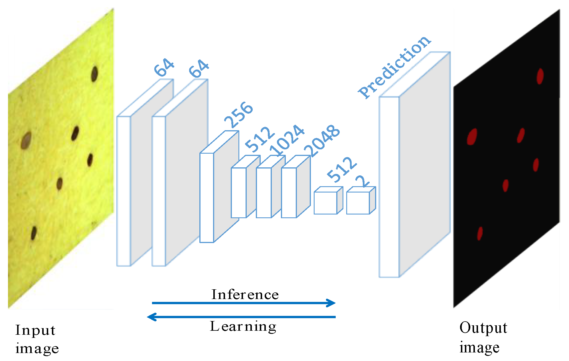
3.1. Deep Learning Analysis of Sand Images

In order to train models conveniently, the resolution of the dataset was uniformly adjusted from 1920 × 1440 to 736 × 736, and the training, validation, and test sets were divided according to a ratio of approximately 6:2:2, after expanding the dataset. The specific dataset division is shown in

Table 2. Dataset of the sand images.

RGB Images 736 × 736 × 3	Training Data	Validation Data	Test Data	Total
−40 + 70	725	244	246	1215
−70 + 100	724	241	243	1208
−100 + 140	728	249	245	1222
−140 + 400	720	237	234	1191

. The sizes of the sand-images input into the three network models are 736 × 736 × 3 pixels. Experiments were programmed with Python3.8. The training processes of the models were run on a 64-bit Windows workstation with an NVIDIA GeForce GTX 3060 GPU and an Intel Core i7. The memory of the GPU was 12 GB, while that of the CPU was 32 GB.

Figure 9 shows the accuracy and loss-function curves of FCN-ResNet50 in 1000 times’ iteration. Figure 9a shows the accuracy curve for the FCN-ResNet50 learning sand-image. The model’s initial accuracy was 21.05%, and the accuracy increased rapidly in the first 250 rounds. The accuracy increased gradually after the initial iteration, and was maintained at a high level, then tended to be stable, reaching 97.26%. Figure 9b shows the loss-function curve of the FCN-ResNet50 learning sand-image. At the initial stage of iterative training, the decline in loss value was significant, showing that the learning rate was suitable, and the gradient-descent process was conducted. After learning to a specific stage, the loss curve tended to become stable, and finally, the loss value was stabilized at around 0.17 after 1000 iterations.

From these results, we confirmed that, by training the sand-grain data with deep learning, it was possible to segment images with a high accuracy of 97.26% and a low loss-value of 0.17 on the validation set.

3.2. Evaluation of Segmentation Networks

After the training of three segmentation models, the test set was used to evaluate the performance of the models. Here, the effect of models was analyzed from the subjective and objective aspects.

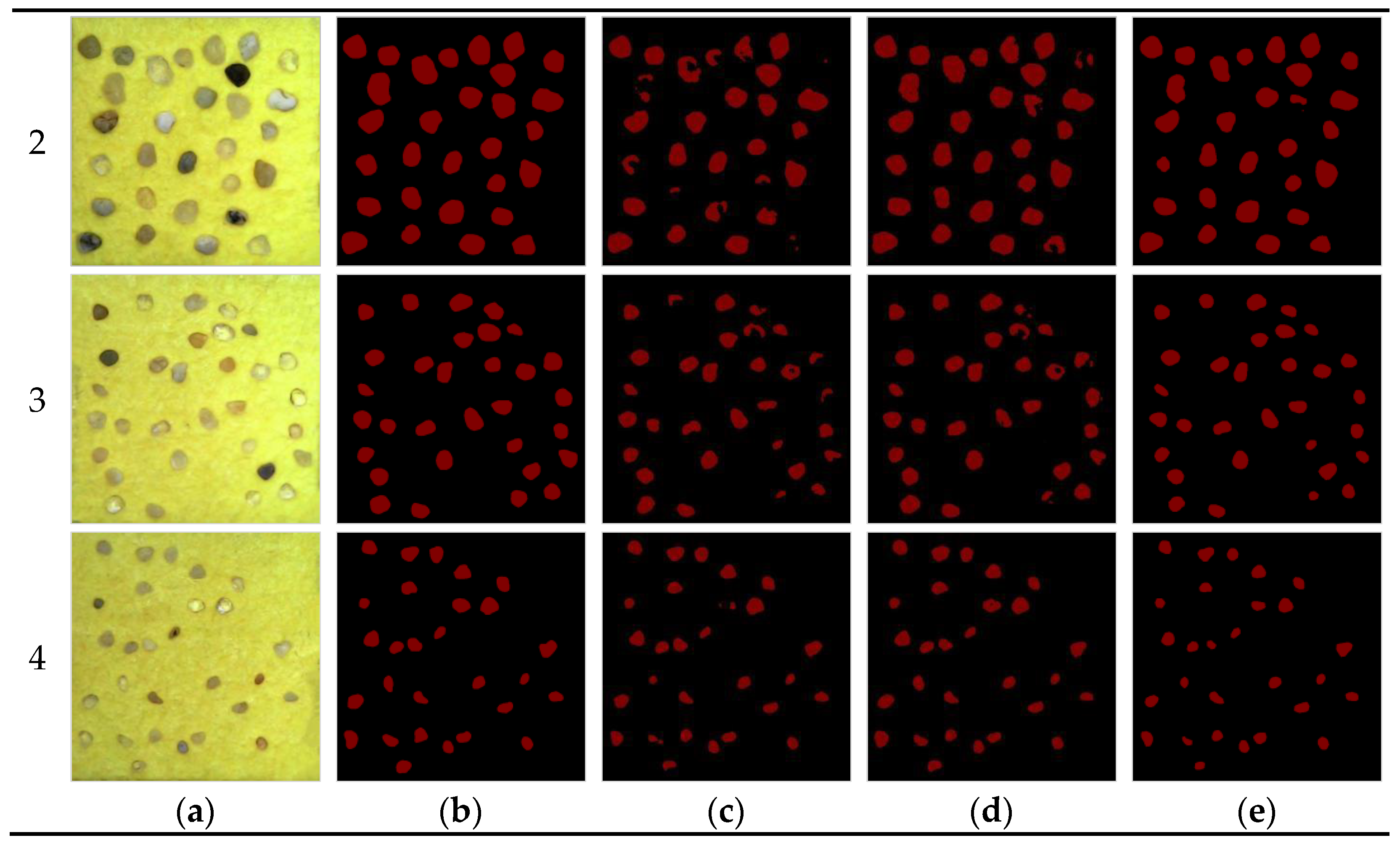
3.2.1. Subjective Analysis of Segmentation Networks

The segmentation effects of the FCN-ResNet50, UNet-Mobile, and Deeplab-Xception deep learning network on four kinds of sand particles were compared intuitively, as shown in Figure 10. The results showed that the FCN-ResNet50 network could more accurately identify each sand particle for quartz sand of −40 + 140 mesh, and the effect was closer to the actual label. The second best was UNet-Mobile, where some sand particles were incomplete and could not be fully identified, whereas the effect of Deeplab-Xception was poor, and transparent sand-particles could not be identified. For −140 + 400 mesh quartz sand, the segmentation effect of UNet-Mobile was the best. However, the three networks were able to identify each sand particle, and the difference between them was slight. In summary, the FCN-ResNet50 network had the best segmentation results for −40 + 140mesh quartz sand; for−140 + 400mesh quartz sand, the effect of the FCN-ResNet50 network was slightly worse than that of the UNet-Mobile and Deeplab-Xception.

3.2.2. Objective Analysis of Segmentation Networks

Intersection over Union (IoU) and Mean Intersection over Union (MIoU) was used to evaluate the model’s segmentation effect in our study. The MIoU is the IoU divided by the number of categories. They are frequently used as evaluation indexes of semantic-segmentation network performance. The merging ratio is the overlap ratio of the predicted and actual values, i.e., the ratio of union and intersection. The ideal case is that the predicted and actual values overlap entirely. The closer the IoU and MIoU get to 1, the better the network segmentation performance. The calculation formula is

$$IoU=\frac{S_{pred}\cap S_{gt}}{S_{pred}\cup S_{gt}},$$

(5)

$$MIoU=\frac{{\displaystyle \sum _{n=1}^{n_{classes}}IoU}}{n_{classes}},$$

(6)

where Spred represents the segmentation network’s predicted label, Sgt represents the actual label, and nclasses represents the number of segmentation categories.

The three segmentation networks calculated the IoU and MIoU of the test sets with four granularities. As can be seen from

Table 3. Objective evaluation index of each model.

Methods	Sand IoU	Background IoU	MIoU
FCN-ResNet50	0.7931	0.9823	0.8877
UNet-Mobile	0.7889	0.9769	0.8829
Deeplab-Xception	0.7704	0.9636	0.8670

, the FCN-ResNet50 network had higher IoU and MIoU than the other two networks, followed by UNet-Mobile, and Deeplab-Xception had poor segmentation performance. In summary, the FCN-ResNet50 network had the best segmentation performance.

3.3. Granularity Measurement

Four quartz-sand images with different grain sizes were put into the FCN-ResNet50, UNet-Mobile, and Deeplab-Xception networks, to generate the segmentation map with black-and-white labels. The sand represents black pixels, and the background represents white pixels. The proportion of black-and-white pixels was calculated, obtaining the pixel-area ratio of sand and background. The pixel-particle size was converted to a physical particle size. Since the sand particles were always in a square frame calibrated by 5 mm in the shooting process, it was easy to obtain the average sand-particle size in the entire image from the total sand-particle area.

The particle-size-detection results of the three networks were compared with the results of manual particle-size calibration-software. Figure 11 shows that the results of FCN-ResNet50 for −40 + 70, −70 + 100, and −100 + 140 mesh quartz-sand particle sizes were the most similar to those of manual particle-size calibration-software, and the gap was the smallest. For the quartz-sand particle size of −140 + 400 mesh, the gap between the results of FCN-ResNet50 and manual particle-size calibration-software was slightly larger than that of UNet-Mobile and Deeplab-Xception. Meanwhile, the errors of each deep learning network in the particle-size detection of quartz sand were further analyzed. The average error of FCN-ResNet50 in the grain-size detection of four grain sizes of quartz sand was the smallest (0.009 mm), meeting the accuracy requirement of quantitative analysis of quartz-sand grain size.

Based on the above results, FCN-ResNet50 had better detection results on coarse-grained sands and a slightly worse effect on fine-grained sands; however, the overall detection results were better. FCN-ResNet50 was the preferred method for granularity measurement.

4. Conclusions

This study used a method based on a deep learning semantic-segmentation network to detect the particle size of quartz sand. A total of 4836 quartz-sand dataset images with a particle size of −40 + 70, −70 + 100, −100 + 140, and −140 + 400 meshes were created. The three models of FCN-ResNet50, UNet-Mobile and Deeplab-Xception were used to segment the quartz sand at the pixel level. tTe segmentation map obtained by the network was then converted into a black and white image, and the final particle size was obtained by converting the pixel size to the physical size.

The results showed that: (1) the accuracy and loss curves of the FCN-ResNet50 model in the training process converged quickly after iteration. The verification accuracy was 97.26 %, and the loss value was 0.17. (2) The IoU and MIoU of the FCN-ResNet50 model were higher than those of the UNet-Mobile and Deeplab-Xception. Considering training efficiency and segmentation accuracy, the FCN-ResNet50 model was the preferred method for quartz-sand segmentation. (3) The particle size of quartz sand measured by the FCN-ResNet50 model was close to the result of the artificial-particle-size calibration-software. The semantic-segmentation method based on deep learning met the accuracy requirements of the quantitative analysis of quartz-sand particle size.

In future work, we can use semi-supervised learning or unsupervised learning to train the model to reduce the dependence of model training on manual labeling and accelerate the analysis and processing of related visual tasks.

References

1. Aripova, M.K.; Mkrtchyan, R.V.; Érkinov, F.B. On the Possibility of Enriching Quartz Raw Materials of Uzbekistan for the Glass Industry. Glass Ceram. 2021, 78, 120–124. [Google Scholar] [CrossRef]
2. Pivinskii, Y.E. Half-Century Epoch of Domestic Quartz Ceramic Development. Part 31. Refract. Ind. Ceram. 2018, 58, 507–513. [Google Scholar] [CrossRef]
3. Klimenko, N.N.; Kolokol’chikov, I.Y.; Mikhailenko, N.Y.; Orlova, L.A.; Sigaev, V.N. New High-Strength Building Materials Based on Metallurgy Wastes. Glass Ceram. 2018, 75, 206–210. [Google Scholar] [CrossRef]
4. Czuryłowicz, K.; Lejzerowicz, A.; Kowalczyk, S.; Wysocka, A. The origin and depositional architecture of Paleogene quartz-glauconite sands in the Lubartów area, eastern Poland. Geol. Q. 2014, 58, 125–144. [Google Scholar]
5. Casalino, G.; De Filippis, L.A.C.; Ludovico, A. A Technical Note on the Mechanical and Physical Characterization of Selective Laser Sintered Sand for Rapid Casting. J. Mater. Process. Technol. 2005, 166, 1–8. [Google Scholar] [CrossRef]
6. Yu, C.; Pu, K.; Geng, R.; Qiao, D.; Lin, D.; Xu, N.; Wang, X.; Li, J.; Gong, S.; Zhou, Q. Comparison of Flip-Flow Screen and Circular Vibrating Screen Vibratory Sieving Processes for Sticky Fine Particles. Miner. Eng. 2022, 187, 107791. [Google Scholar] [CrossRef]
7. Xie, H.; Liu, R.; Li, Y.; Zhang, P.; Ding, C.; Chen, L.; Tong, X. The Application of a New Type of Hydraulic Classification Equipment: Swirl Continuous Centrifugal Separator. In Proceedings of the ACMME 2017, Xishuangbanna, China, 20–21 May 2017. [Google Scholar]
8. Polakowski, C.; Ryżak, M.; Sochan, A.; Beczek, M.; Mazur, R.; Bieganowski, A. Particle Size Distribution of Various Soil Materials Measured by Laser Diffraction—The Problem of Reproducibility. Minerals 2021, 11, 465. [Google Scholar] [CrossRef]
9. Bals, J.; Loza, K.; Epple, P.; Kircher, T.; Epple, M. Automated and Manual Classification of Metallic Nanoparticles with Respect to Size and Shape by Analysis of Scanning Electron Micrographs. Mater. Und Werkst. 2022, 53, 270–283. [Google Scholar] [CrossRef]
10. Ye, R.Q.; Niu, R.Q.; Zhang, L.P. Mineral Features Extraction and Analysis Based on Multiresolution Segmentation of Petrographic Images. J. Jilin Univ. (Earth Sci. Ed.) 2011, 41, 1253–1261. (In Chinese) [Google Scholar]
11. Köse, C.; Alp, İ.; İkibaş, C. Statistical Methods for Segmentation and Quantification of Minerals in Ore Microscopy. Miner. Eng. 2012, 30, 19–32. [Google Scholar] [CrossRef]
12. Suprunenko, V.V. Ore Particles Segmentation Using Deep Learning Methods. In Proceedings of the APITECH 2020, Krasnoyarsk, Russia, 25 September–4 October 2020. [Google Scholar]
13. Filippo, M.P.; Gomes, O.D.F.M.; da Costa, G.A.O.P.; Mota, G.L.A. Deep Learning Semantic Segmentation of Opaque and Non-Opaque Minerals From Epoxy Resin in Reflected Light Microscopy Images. Miner. Eng. 2021, 170, 107007. [Google Scholar]
14. Liu, X.; Zhang, Y.; Jing, H.; Wang, L.; Zhao, S. Ore Image Segmentation Method Using U-Net and Res_Unet Convolutional Networks. RSC Adv. 2020, 10, 9396–9406. [Google Scholar] [CrossRef] [Green Version]
15. Sun, G.; Huang, D.; Cheng, L.; Jia, J.; Xiong, C.; Zhang, Y. Efficient and Lightweight Framework for Real-Time Ore Image Segmentation Based on Deep Learning. Minerals 2022, 12, 526. [Google Scholar] [CrossRef]
16. Duan, J.; Liu, X.; Wu, X.; Mao, C. Detection and Segmentation of Iron Ore Green Pellets in Images Using Lightweight U-Net Deep Learning Network. Neural Comput. Appl. 2020, 32, 5775–5790. [Google Scholar] [CrossRef]
17. Wang, Y.; Bai, X.; Wu, L.; Zhang, Y.; Qu, S. Identification of Maceral Groups in Chinese Bituminous Coals Based on Semantic Segmentation Modelso. Fuel 2022, 308, 121844. [Google Scholar] [CrossRef]
18. Long, J.; Shelhamer, E.; Darrell, T. Fully Convolutional Networks for Semantic Segmentation. In Proceedings of the CVPR 2015, Boston, MA, USA, 7–12 June 2015. [Google Scholar]
19. He, K.; Zhang, X.; Ren, S.; Sun, J. Deep Residual Learning for Image Recognition. In Proceedings of the CVPR 2016, Seattle, WA, USA, 27–30 June 2016. [Google Scholar]
20. Ronneberger, O.; Fischer, P.; Brox, T. U-Net: Convolutional Networks for Biomedical Image Segmentation. In Proceedings of the MICCAI 2015, Munich, Germany, 5–9 October 2015. [Google Scholar]
21. Howard, A.G.; Zhu, M.; Chen, B.; Kalenichenko, D.; Wang, W.; Weyand, T.; Andreetto, M.; Adam, H. MobileNets: Efficient Convolutional Neural Networks for Mobile Vision Applications. arXiv 2017, arXiv:1704.04861. [Google Scholar]
22. Chen, L.C.; Papandreou, G.; Kokkinos, I.; Murphy, K.; Yuille, A.L. Deeplab: Semantic Image Segmentation with Deep Convolutional Nets, Atrous convolution, and Fully Connected Crfs. IEEE Trans. Pattern Anal. Mach. Intell. 2017, 40, 834–848. [Google Scholar] [CrossRef] [Green Version]
23. Chollet, F. Xception: Deep Learning with Depthwise Separable Convolutions. In Proceedings of the CVPR 2017, Honolulu, HI, USA, 21–26 July 2017. [Google Scholar]
24. Shi, L.; Li, B.; Kim, C.; Kellnhofer, P.; Matusik, W. Towards Real-Time Photorealistic 3D Holography with Deep Neural Networks. Nature 2021, 591, 234–239. [Google Scholar] [CrossRef]
25. Reichstein, M.; Camps-Valls, G.; Stevens, B.; Jung, M.; Denzler, J.; Carvalhais, N. Deep Learning and Process Understanding for Data-Driven Earth System Science. Nature 2019, 566, 195–204. [Google Scholar] [CrossRef]
26. Bollu, T.; Ito, B.S.; Whitehead, S.C.; Kardon, B.; Redd, J.; Liu, M.H.; Goldberg, J.H. Cortex-Dependent Corrections as the Tongue Reaches for and Misses Targets. Nature 2021, 594, 82–87. [Google Scholar] [CrossRef]
27. Jing, L.; Tian, Y. Self-Supervised Visual Feature Learning with Deep Neural Networks: A Survey. IEEE Trans. Pattern Anal. Mach. Intell. 2020, 43, 4037–4058. [Google Scholar] [CrossRef]
Figure 1. A diagram of sand-grain images semantic-segmentation network model.
Minerals 12 01479 g001
Figure 2. A diagram of the linear interpolation: (a) single-linear interpolation; (b) bilinear interpolation.
Minerals 12 01479 g002
Figure 3. A diagram of the fully convolutional network (FCN) skip structure.
Minerals 12 01479 g003
Figure 4. A diagram of ResNet50 residual learning.
Minerals 12 01479 g004
Figure 5. A diagram of FCN-ResNet50 network structure.
Minerals 12 01479 g005
Figure 6. A diagram of a camera system.
Minerals 12 01479 g006
Figure 7. Quartz-sand-sample images of four particle sizes: (a) −40 + 70 mesh; (b) −70 + 100 mesh (c) −100 + 140 mesh; (d) −140 + 400 mesh.
Minerals 12 01479 g007
Figure 8. Flow chart of dataset expansion and model prediction.
Minerals 12 01479 g008
Figure 9. Deep learning graph of sand-grain pictures: (a) accuracy curve of FCN-ResNet50, (b) loss-function curve of FCN-ResNet50.
Minerals 12 01479 g009
Figure 10. The segmentation effects of three deep learning networks on four particle sizes of sand (row 1–4 −40 + 70, −70 + 100, −100 + 140, −140 + 400 meshes): (a) original image; (b) ground truth; (c) Deeplab-Xception; (d) UNet-Mobile;(e) FCN-ResNet50.
Minerals 12 01479 g010aMinerals 12 01479 g010b
Figure 11. Comparative and analysis graph of particle size measurement.
Minerals 12 01479 g011