
Discussion on Criterion of Determination of the Kinetic Parameters of the Linear Heating Reactions


Abstract
:1. Introduction
2. Theoretical Models
2.1. Nonisothermal Kinetics
2.2. The Criterion of Determination
2.3. Explicit Euler Method
2.4. Taylor Expansion Method
2.5. Mean Square Error
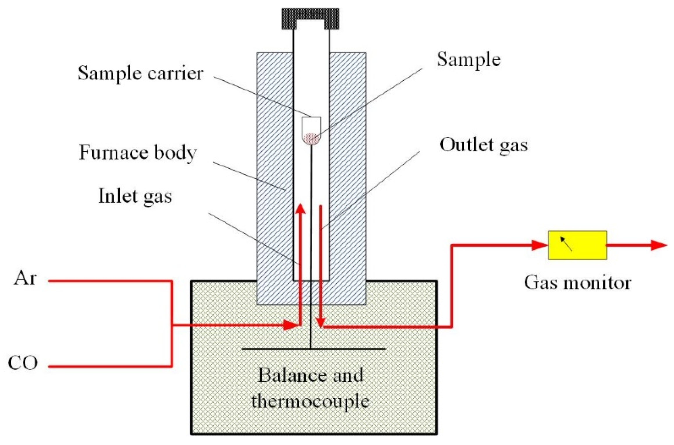
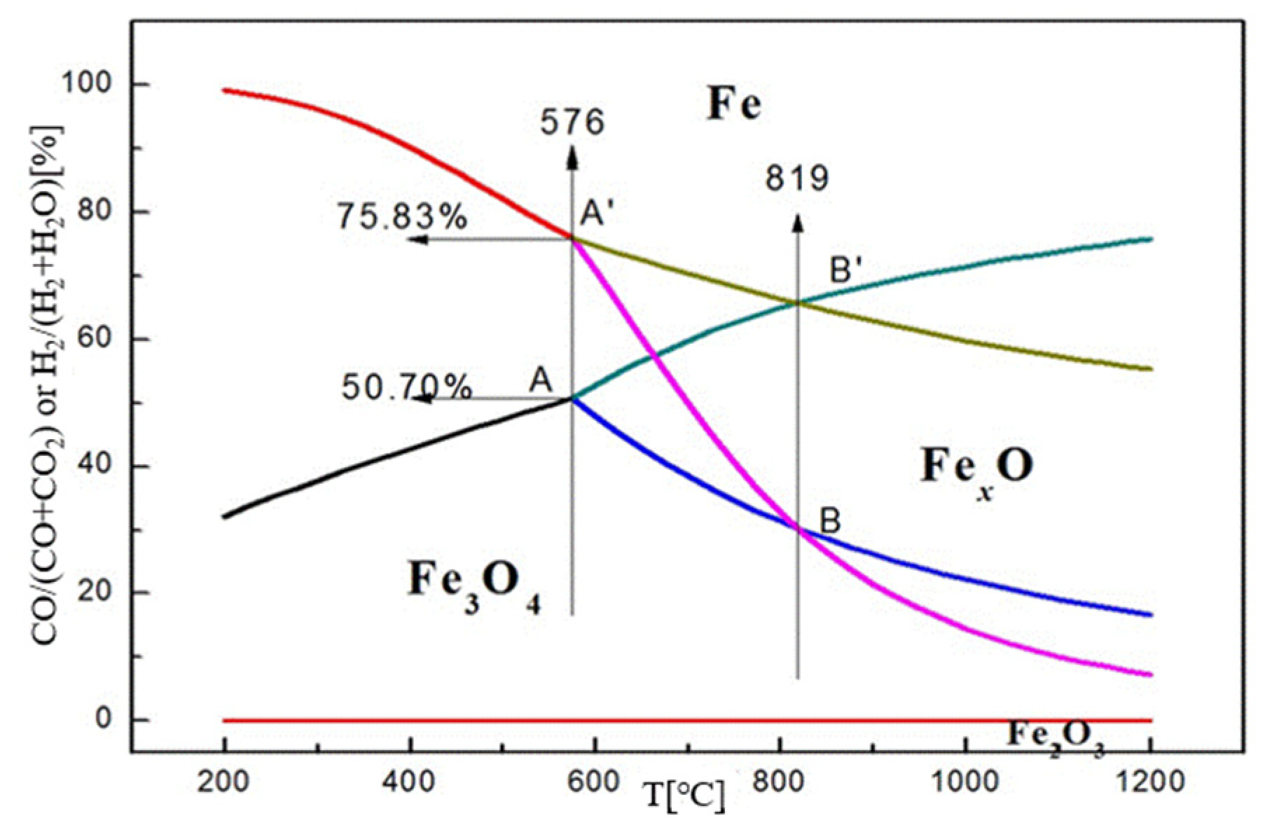
3. Experimental Procedure
4. Results and Discussion
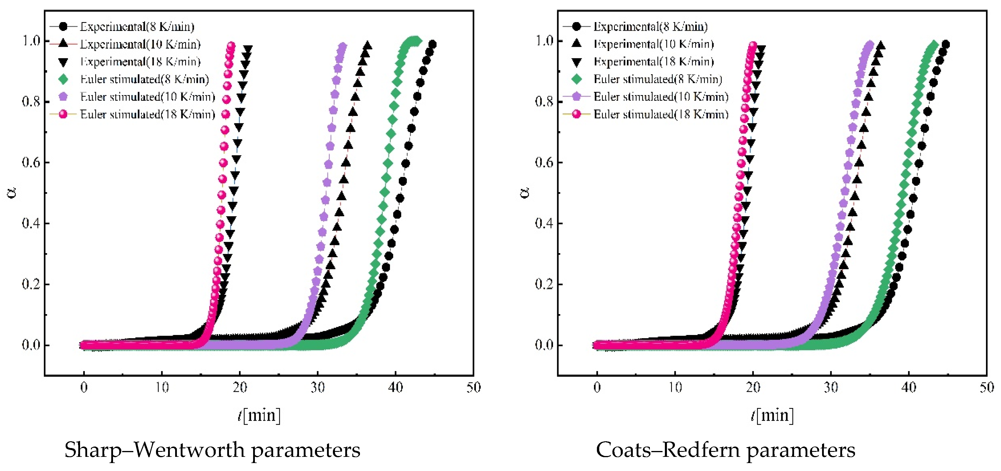
4.1. Fitting Results
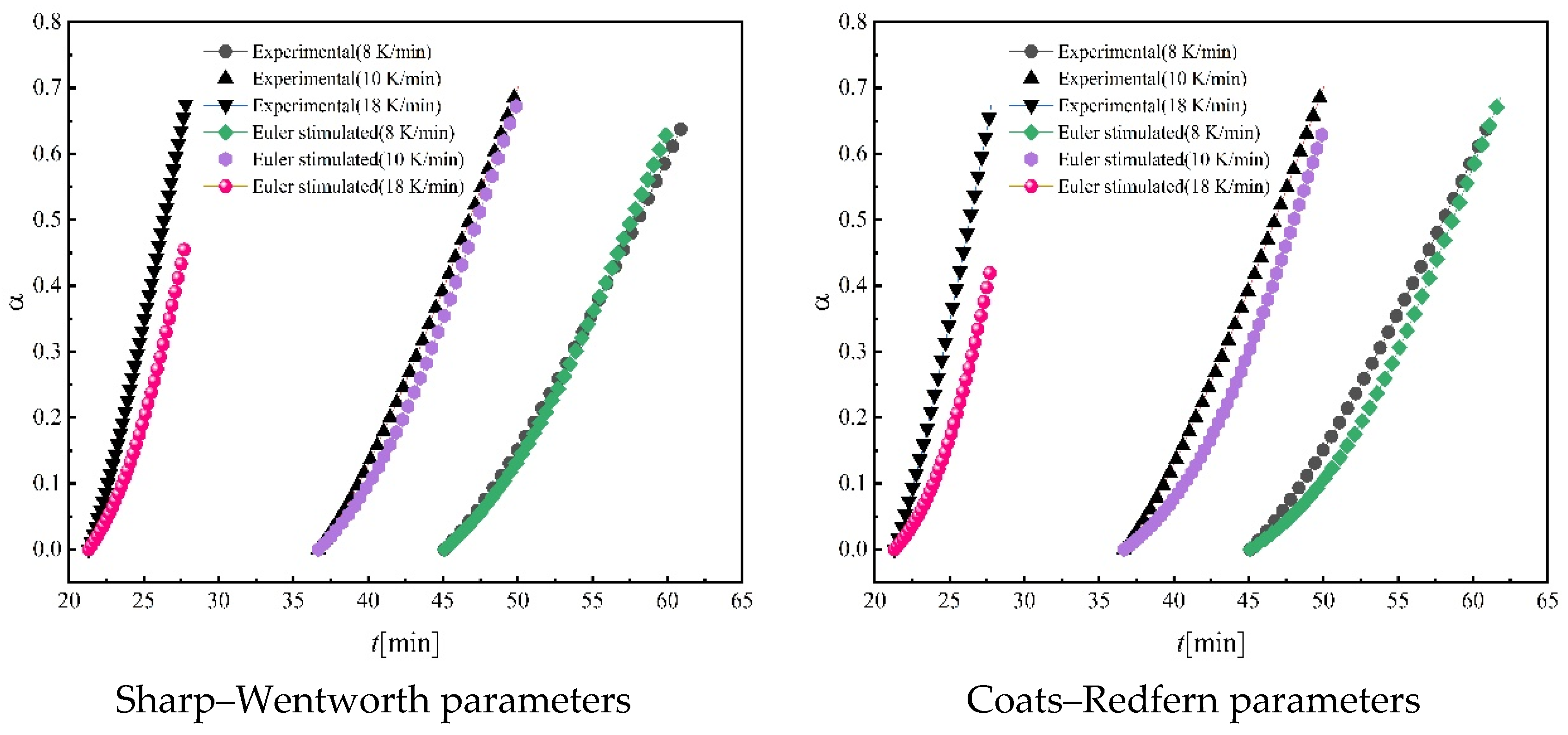
4.2. Results from Explicit Euler Method
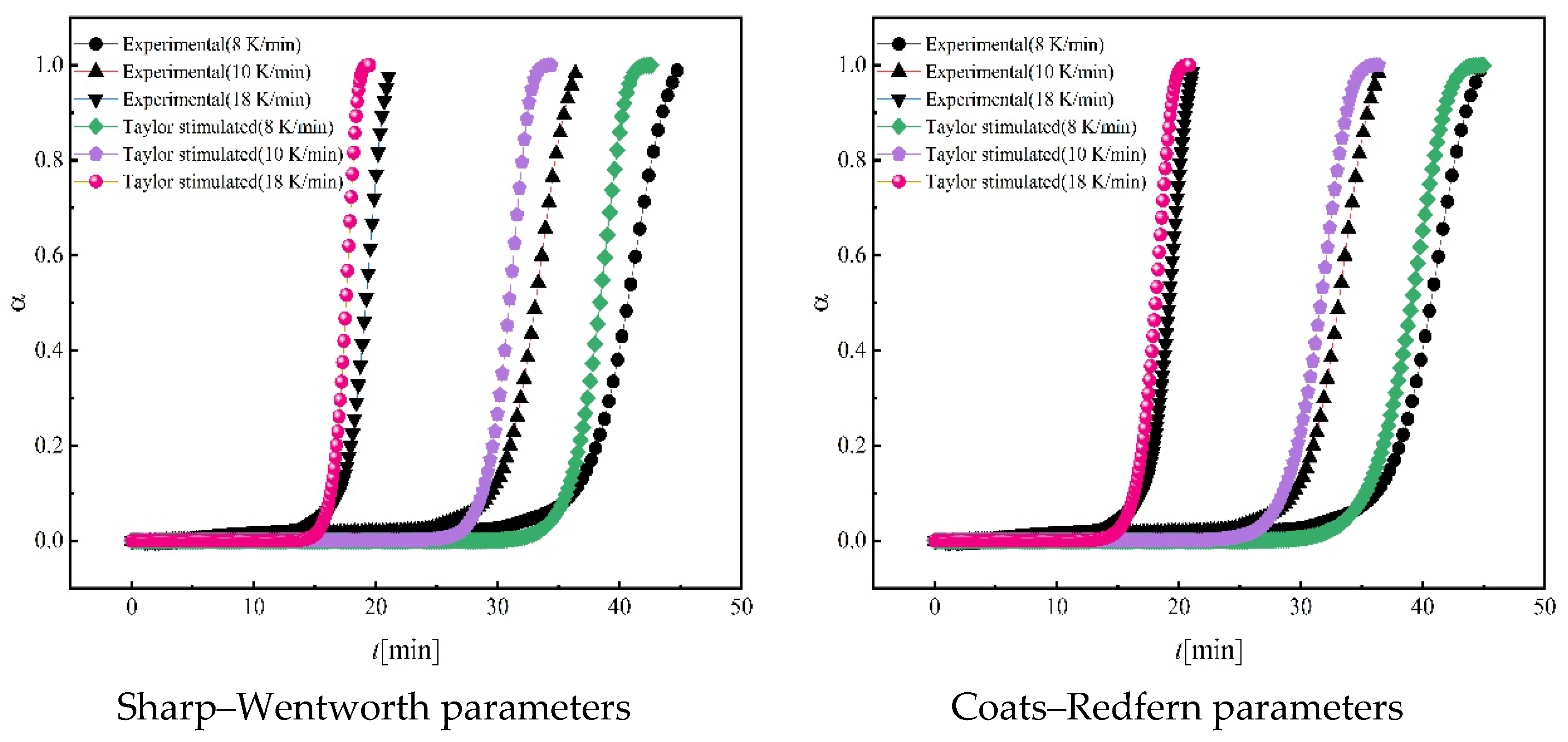
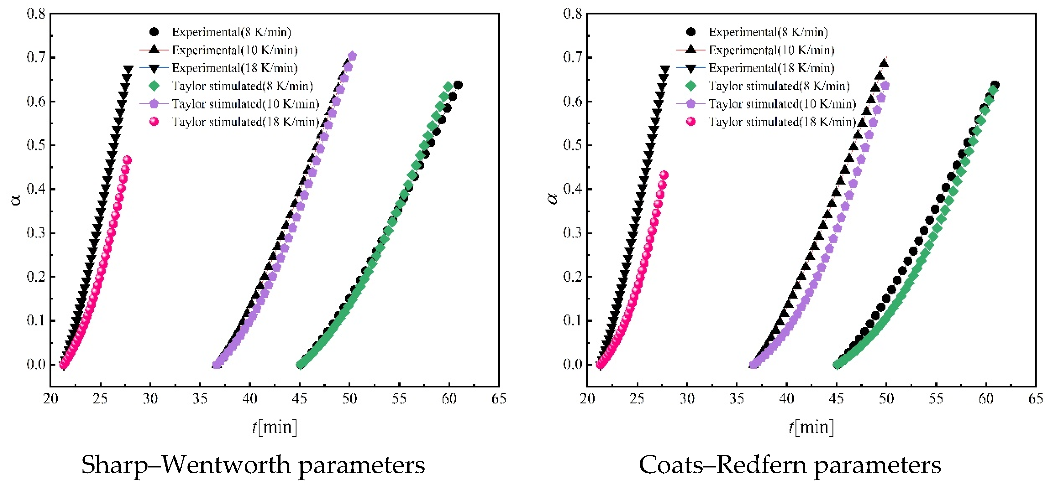
4.3. Results from Taylor Expansion Method
5. Conclusions
Author Contributions
Funding
Acknowledgments
Conflicts of Interest
Abbreviations
| α | Conversion rate | - |
| β | Linear heating rate | K/min |
| b | Total reaction time | min |
| f | Slope | min−1 |
| m | Number of nodes | - |
| t | Reaction time | min |
| h | Step length | min |
| f(α) | Reaction model | - |
| g(α) | The integral form of f(α) | - |
| k(T) | Reaction constant | min−1 |
| A | Pre-exponential factor | min−1 |
| E | Activation energy | J/mol |
| N | Mean squared number of nodesnodes | - |
| T | Reaction temperature | K |
| MSE | Mean square error | - |
| TGA | Thermal gravimetric analyzer | - |
| DSC | Differential scanning calorimetry | - |
| DTA | Differential thermal analysis | - |
References
- Yuan, S.; Zhang, Q.; Yin, H.; Li, Y. Efficient iron recovery from iron tailings using advanced suspension reduction technology: A study of reaction kinetics, phase transformation, and structure evolution. J. Hazard. Mater. 2021, 404, 124067. [Google Scholar] [CrossRef]
- Wan, X.; Shi, J.; Klemettinen, L.; Chen, M.; Taskinen, P.; Jokilaakso, A. Equilibrium phase relations of CaO–SiO2–TiO2 system at 1400 °C and oxygen partial pressure of 10−10 atm. J. Alloys Compd. 2020, 847, 156472. [Google Scholar] [CrossRef]
- Zhang, J.; Zhang, W.; Xue, Z. Oxidation Kinetics of Vanadium Slag Roasting in the Presence of Calcium Oxide. Miner. Process. Extr. Metall. Rev. 2017, 38, 265–273. [Google Scholar] [CrossRef]
- Liu, P.; Liu, C.; Hu, T.; Shi, J.; Zhang, L.; Liu, B.; Peng, J. Kinetic study of microwave enhanced mercury desorption for the regeneration of spent activated carbon supported mercuric chloride catalysts. Chem. Eng. J. 2021, 408, 127355. [Google Scholar] [CrossRef]
- Peng, X.; Liu, W.; Liu, W.; Zhao, L.; Zhang, N.; Gu, X.; Zhou, S. Fluorite enhanced magnesium recovery from serpentine tailings: Kinetics and reaction mechanisms. Hydrometallurgy 2021, 201, 105571. [Google Scholar] [CrossRef]
- Zhang, W.; Dai, J.; Li, C.; Yu, X.; Xue, Z.; Saxén, H. A Review on Explorations of the Oxygen Blast Furnace Process. Steel Res. Int. 2021, 92, 1–23. [Google Scholar] [CrossRef]
- Coats, A.W.; Redfern, J.P. Kinetic parameters from thermogravimetric data. Nature 1964, 201, 68–69. [Google Scholar] [CrossRef]
- Freeman, E.; Carroll, B. The application of thermoanalytical techniques to kinetics: The thermogravimetric evaluation of the kinetics of the decomposition of calcium oxalate monohydrate. J. Phys. Chem. 1975, 62, 394–397. [Google Scholar] [CrossRef]
- Wang, T.X.; Ding, C.Y.; Lv, X.W.; Xuan, S.W.; Li, G. Reduction kinetics of MgO-doped calcium ferrites under CO–N2 atmosphere. J. Iron Steel Res. Int. 2019, 26, 1265–1272. [Google Scholar] [CrossRef]
- Huang, Z.C.; Wu, K.; Hu, B.; Peng, H.; Jiang, T. Non-Isothermal Kinetics of Reduction Reaction of Oxidized Pellet Under Microwave Irradiation. J. Iron Steel Res. Int. 2012, 19, 1–4. [Google Scholar] [CrossRef]
- Han, G.H.; Jiang, T.; Zhang, Y.B.; Huang, Y.F.; Li, G.H. High-temperature oxidation behavior of vanadium, titanium-bearing magnetite pellet. J. Iron Steel Res. Int. 2011, 18, 14–19. [Google Scholar] [CrossRef]
- Vyazovkin, S.; Wight, C.A. Model-free and model-fitting approaches to kinetic analysis of isothermal and nonisothermal data. Thermochim. Acta 1999, 340–341, 53–68. [Google Scholar] [CrossRef]
- Darken, L.S.; Gurry, R.W. The System Iron-Oxygen. I. The Wüstite Field and Related Equilibria. J. Am. Chem. Soc. 1945, 67, 1398–1412. [Google Scholar] [CrossRef]
- Xing, L.Y.; Zou, Z.S.; Qu, Y.X.; Shao, L.; Zou, J.Q. Gas–Solid Reduction Behavior of In-flight Fine Hematite Ore Particles by Hydrogen. Steel Res. Int. 2019, 90, 1–10. [Google Scholar] [CrossRef] [Green Version]
- Zheng, H.; Schenk, J.; Spreitzer, D.; Wolfinger, T.; Daghagheleh, O. Review on the Oxidation Behaviors and Kinetics of Magnetite in Particle Scale. Steel Res. Int. 2021, 92, 1–13. [Google Scholar] [CrossRef]
- Pei, Z.; Peimin, G.; Dianwei, Z. study on reduction sequenece of hematite at low-temperature non-equilibrium state. Iorn Steel 2006, 41, 12–15. [Google Scholar]
- Wimmers, O.J.; Arnoldy, P.; Moulijn, J.A. Determination of the reduction mechanism by temperature-programmed reduction: Application to small Fe2O3 particles. J. Phys. Chem. 1986, 90, 1331–1337. [Google Scholar] [CrossRef]
- Zhang, W.; Zhang, J.H.; Zou, Z.S.; Li, Q.; Qi, Y.H. Influences of non-stoichiometry on thermodynamics and kinetics of iron oxides reduction processes. Ironmak. Steelmak. 2014, 41, 715–720. [Google Scholar] [CrossRef]
- Hedvall, J.A. Reaktionsfähigkeit Fester Stoffe. Angew. Chem. 1938, 51, 150. [Google Scholar] [CrossRef]
- Garner, W.E. Chemistry of the Solid State; Butterworths Scientific Publications: London, UK, 1955. [Google Scholar] [CrossRef] [Green Version]
- Jost, W. Diffusion und Chemische Reaktionen in Festen Stoffen. Nature 1938, 142, 776. [Google Scholar] [CrossRef]
- Vyazovkin, S.; Burnham, A.K.; Criado, J.M.; Pérez-Maqueda, L.A.; Popescu, C.; Sbirrazzuoli, N. ICTAC Kinetics Committee recommendations for performing kinetic computations on thermal analysis data. Thermochim. Acta 2011, 520, 1–19. [Google Scholar] [CrossRef]
- Han, Y.; Li, T.; Saito, K. Comprehensive method based on model free method and IKP method for evaluating kinetic parameters of solid state reactions. J. Comput. Chem. 2012, 33, 2516–2525. [Google Scholar] [CrossRef]
- Sharp, J.H.; Wentworth, S.A. Kinetic analysis of thermogravimetric data. Anal. Chem. 1969, 41, 2060–2062. [Google Scholar] [CrossRef]
- Ozawa, T. Kinetic analysis of derivative curves in thermal analysis. J. Therm. Anal. 1970, 2, 301–324. [Google Scholar] [CrossRef]
- Sestak, J.; Satava, V.; Wendlandt, W.W. The study of heterogeneous processes by thermal analysis. Thermochim. Acta 1973, 7, 333–556. [Google Scholar] [CrossRef]
- Vyazovkin, S. Model-free kinetics: Staying free of multiplying entities without necessity. J. Therm. Anal. Calorim. 2006, 83, 45–51. [Google Scholar] [CrossRef]
- Glasstone, K.S.; Laidler, J.; Eyring, H. The Theory of Rate Processes. Nature 1941, 149, 509–510. [Google Scholar]
- Galwey, A.K.; Brown, M. Thermal Decomposition of Ionic Solids; Elsevier Science: Amsterdam, The Netherlands, 1999. [Google Scholar]
- Brown, M.E.; Dollimore, D.; Galwey, A.K. Comprehensive Chemical Kinetics.Reactions in the Solid State; Elsevier: Amsterdam, The Netherlands, 1980; Volume 22. [Google Scholar]
- Sardari, A.; Alamdari, E.K.; Noaparast, M.; Shafaei, S.Z. Kinetics of magnetite oxidation under non-isothermal conditions. Int. J. Miner. Metall. Mater. 2017, 24, 486–492. [Google Scholar] [CrossRef]
- Barile, C.; Casavola, C.; Vimalathithan, P.K.; Pugliese, M.; Maiorano, V. Thermomechanical and morphological studies of CFRP tested in different environmental conditions. Materials 2018, 12, 63. [Google Scholar] [CrossRef] [Green Version]
- Wang, F.; Qian, D.S.; Xiao, P.; Deng, S. Accelerating cementite precipitation during the non-isothermal process by applying tensile stress in GCr15 bearing steel. Materials 2018, 11, 2403. [Google Scholar] [CrossRef] [Green Version]
- Johnson, N.L.; Leone, F.C. Statistics and Experimental Design in Engineering and the Physical Sciences; Wiley: New York, NY, USA, 1977. [Google Scholar]
- Harnett, D.L. Statistical Methods; Addison-Wesley: Reading, UK, 1982. [Google Scholar]
- Draper, N.R.; Smith, H. Applied Regression Analysis; Wiley: New York, NY, USA, 1981. [Google Scholar]
- Vyazovkin, S.; Wight, C.A. Isothermal and nonisothermal reaction kinetics in solids: In search of ways toward consensus. J. Phys. Chem. A 1997, 101, 8279–8284. [Google Scholar] [CrossRef]
- Zhang, W.; Zhang, J.; Li, Q.; He, Y.; Tang, B.; Li, M.; Zhang, Z.; Zou, Z. Thermodynamic analyses of iron oxides redox reactions. In Proceedings of the 8th Pacific Rim International Congress on Advanced Materials and Processing, PRICM 8, Waikoloa, HI, USA, 4–9 August 2013; Marquis, F., Ed.; Wiley: Waikoloa, HI, USA, 2013; pp. 777–789. [Google Scholar]


| Reaction Model | Code | |||
|---|---|---|---|---|
| 1 | Power law | p4 | 4α3/4 | α1/4 |
| 2 | Power law | P3 | 3α2/3 | α1/3 |
| 3 | Power law | P2 | 2α1/2 | α1/2 |
| 4 | Power law | P2/3 | 2/3α−1/2 | α3/2 |
| 5 | One-dimensional diffusion | D1 | 1/2α-l | α2 |
| 6 | Mampel (first order) | F1 | 1 − α | −ln(1 − α) |
| 7 | Awrami-Erofeev | A4 | 4(1 − α)[−ln(1 − α)]3/4 | [−ln(1 − α)]1/4 |
| 8 | Avrami-Erofeev | A3 | 3(1 − α)[−ln(1 − α)]2/3 | [−ln(1 − α)]1/3 |
| 9 | Avrami-Erofeev | A2 | 2(1 − α)[−ln(1 − α)]1/2 | [−ln(1 − α)]1/2 |
| 10 | Three-dimensional diffusion | D3 | 3/2(1 − α)2/3[1 − (1 − α)1/3]−1 | [1 − (1 − α)1/3]2 |
| 11 | Contracting sphere | R3 | 3(1 − α)2/3 | 1 − (1 − α)1/3 |
| 12 | Contracting cylinder | R2 | 2(1 − α)1/2 | 1 − (1 − α)1/2 |
| 13 | Two-dimensional diffusion | D2 | [−ln(1 − α)]−1 | (1 − α)ln(1 − α) + α |
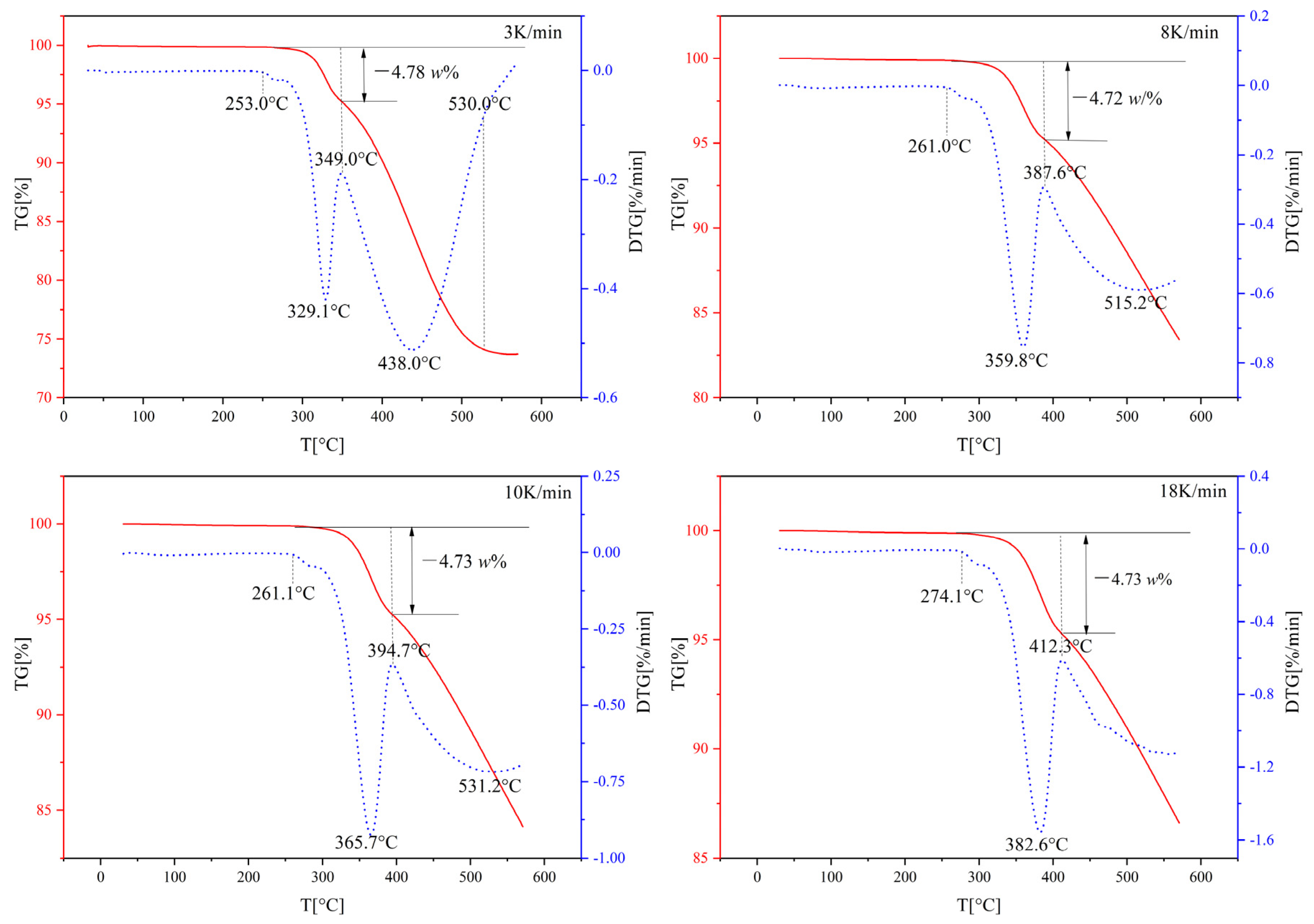
| Heating Rate/(K/min) | Fe2O3 → Fe3O4 (°C) | Fe3O4 → Fe (°C) |
|---|---|---|
| 3 | 253.0–329.1 | 329.1–520.0 |
| 8 | 261.0–387.6 | 387.6–520.0 |
| 10 | 261.1–394.7 | 394.7–520.0 |
| 18 | 274.1–412.3 | 412.3–520.0 |
| Sharp–Wentworth | Coats–Redfern | |||||||
|---|---|---|---|---|---|---|---|---|
| β/(K/min) | E (J/mol) | Reaction Order | ln (A/min) | r2 | E (J/mol) | Reaction Order | ln (A/min) | r2 |
| 3 | 246,385 | First | 47.68 | 0.9992 | 176,498 | First | 33.28 | 0.9857 |
| 8 | 179,333 | First | 35.25 | 0.9994 | 144,763 | First | 26.37 | 0.9875 |
| 10 | 179,316 | First | 35.35 | 0.9989 | 147,216 | First | 26.78 | 0.9906 |
| 18 | 171,360 | First | 34.15 | 0.9981 | 132,533 | First | 23.81 | 0.9796 |
| Sharp–Wentworth | Coats–Redfern | |||||||
|---|---|---|---|---|---|---|---|---|
| β/(K/min) | E (J/mol) | Reaction Order | ln (A/min) | r2 | E (J/mol) | Reaction Order | ln (A/min) | r2 |
| 3 | 72,576 | First | 9.28 | 0.9994 | 81,382 | First | 10.57 | 0.9984 |
| 8 | 56,040 | First | 6.48 | 0.9969 | 142,386 | Third | 21.39 | 0.9908 |
| 10 | 58,440 | First | 7.32 | 0.9919 | 147,765 | Third | 22.38 | 0.9917 |
| 18 | 63,649 | First | 8.44 | 0.9941 | 171,202 | Third | 26.53 | 0.9933 |
| Sharp–Wentworth | Coats–Redfern | |||||
|---|---|---|---|---|---|---|
| β | 8 K/min | 10 K/min | 18 K/min | 8 K/min | 10 K/min | 18 K/min |
| N | 70 | 65 | 53 | 70 | 65 | 53 |
| MSE | 0.0463 | 0.0563 | 0.0720 | 0.0171 | 0.0174 | 0.0191 |
| Sharp–Wentworth | Coats–Redfern | |||||
|---|---|---|---|---|---|---|
| β | 8 K/min | 10 K/min | 18 K/min | 8 K/min | 10 K/min | 18 K/min |
| N | 83 | 88 | 66 | 83 | 88 | 66 |
| MSE | 0.0003 | 0.0013 | 0.0185 | 0.0019 | 0.0054 | 0.0262 |
| Sharp–Wentworth | Coats–Redfern | |||||
|---|---|---|---|---|---|---|
| β | 8 K/min | 10 K/min | 18 K/min | 8 K/min | 10 K/min | 18 K/min |
| N | 70 | 65 | 53 | 70 | 65 | 53 |
| MSE | 0.0531 | 0.0618 | 0.0873 | 0.0200 | 0.0213 | 0.0264 |
| Sharp–Wentworth | Coats–Redfern | |||||
|---|---|---|---|---|---|---|
| β | 8 K/min | 10 K/min | 18 K/min | 8 K/min | 10 K/min | 18 K/min |
| N | 70 | 65 | 53 | 70 | 65 | 53 |
| MSE | 0.0003 | 0.0010 | 0.0166 | 0.0016 | 0.0047 | 0.0238 |
Publisher’s Note: MDPI stays neutral with regard to jurisdictional claims in published maps and institutional affiliations. |
© 2022 by the authors. Licensee MDPI, Basel, Switzerland. This article is an open access article distributed under the terms and conditions of the Creative Commons Attribution (CC BY) license (https://creativecommons.org/licenses/by/4.0/).
Share and Cite
Li, K.; Zhang, W.; Fu, M.; Li, C.; Xue, Z. Discussion on Criterion of Determination of the Kinetic Parameters of the Linear Heating Reactions. Minerals 2022, 12, 81. https://doi.org/10.3390/min12010081
Li K, Zhang W, Fu M, Li C, Xue Z. Discussion on Criterion of Determination of the Kinetic Parameters of the Linear Heating Reactions. Minerals. 2022; 12(1):81. https://doi.org/10.3390/min12010081
Chicago/Turabian StyleLi, Kui, Wei Zhang, Menglong Fu, Chengzhi Li, and Zhengliang Xue. 2022. "Discussion on Criterion of Determination of the Kinetic Parameters of the Linear Heating Reactions" Minerals 12, no. 1: 81. https://doi.org/10.3390/min12010081