Study of the Influence of Non-Deposit Locations in Data-Driven Mineral Prospectivity Mapping: A Case Study on the Iskut Project in Northwestern British Columbia, Canada

Abstract

The accuracy of data-driven predictive mineral prospectivity models relies heavily on the training datasets used. These models are usually trained using data for “known” deposit locations as well as “non-deposit” locations that are based on randomly generated point patterns. In this study, data related to the Seabridge Gold Inc Iskut project, an epithermal Au deposit in northwestern British Columbia (BC), Canada, are used to test the utility of data-driven mineral prospectivity modeling. The input spatial dataset is comprised mostly of publicly available data. Data for 18 vein and epithermal Au known mineral occurrences (KMO) are obtained from the BC Geological Survey’s MINFILE repository and selected as training deposit locations. A total of eleven sets of non-deposit locations (NDL) were also created, including one set of selected non-prospective KMO for Au deposits from the MINFILE and ten sets of random point patterns. Given the scale of this study, most of the KMO recorded on the property are of the epithermal deposit type. Hence, they could not be used as a selection criterion. Data-driven mineral potential models are generated using the random forest (RF) algorithm and trained on multiple data sets. The comparison of RF models demonstrated that using non-prospective KMO generates more accurate predictions than the random point pattern. The produced mineral prospectivity maps delineated multiple areas with higher discovery potential, which matched viable targets for the Au-Cu epithermal-porphyry system identified through previous Seabridge Gold Inc. (Toronto, ON, Canada) field reconnaissance and drilling programs.

1. Introduction

With new mineral deposits becoming more challenging to find, geoscientists have focused on development of novel methods to assist with mineral deposit discovery. Development of the geographic information system (GIS) technology, improved computing power, and application of data-driven methods, such as machine learning, are enabling the evolution of quantitative methods of geoscientific data analysis, including mineral potential mapping (MPM) [1,2]. For instance, in 2018, Goldcorp Inc., Vancouver, BC, Canada (now part of the Newmont Corporation) and IBM announced a partnership with a goal to utilize the IBM Watson supercomputer and its artificial intelligence (AI) framework to aid mineral targeting at the Red Lake Mines in northwestern Ontario, Canada.

MPM consists of combining multiple layers of geoscience data into a map identifying areas favorable for mineral exploration. The process can be summarized into five main steps: definition of the exploration model for the type of deposit sought, selection of the geospatial dataset to be used, processing of data, creation of the predictor maps, integration of the predictor maps to create a predictive model [1,2].

There are three main categories of modeling methods using GIS-environment: knowledge-driven, data-driven and hybrid.

The knowledge-driven approach requires “experts” to assign weights and to assess the relative importance of each evidential layer as they relate to the specific exploration model being used. This method is subjective but has the advantage of being well suited for greenfield areas with missing or scarce data and where few deposits are known [3]. Examples of knowledge-driven approach include Boolean logic [1,2,4], index overlays [1,2,4,5], fuzzy logic [6,7,8,9,10] and evidential belief [2,6].

The data-driven approach uses the spatial relationship between the geospatial features and known mineral deposits (training set) to estimate the model parameters. It is well suited for well-established mining areas where a large number of known mineral deposits is available to quantify the spatial associations with evidential features and to guarantee the performance and robustness of the model. Methods such as weights of evidence [4,7,11,12,13], logistic regression [11,12], neural networks [11,14,15], support vector machine [15,16,17,18] and random forest [3,13,19,20,21,22] are examples of data-driven approaches.

Since 2000, the number of publications on data-driven methods for MPM has largely increased, especially articles using machine learning algorithms (MLA) [23]. In recent years, the random forest (RF) algorithm has proven to offer a new approach to MPM. Contrarily to other MLA, like artificial neural networks or support vector machine, RF is not a ‘black-box’ algorithm, meaning that the inner workings of the algorithm are known and can even be represented (i.e., decision trees). It is also simpler to parameterize, more stable and computationally light [15,22,24,25].

For any data-driven method, the training dataset should contain a sufficient number of samples to train a given model, and studies showed that RF can be accurate even with a small training set (i.e., less than 20 deposit locations) [19,20,24,26,27]. Moreover, the training dataset should be balanced, meaning that the dataset must contain an equal number of deposits and non-deposit, to avoid results to be biased for one class or the other [19]. Training deposit locations are usually discovered deposits or known mineral occurrences (KMO) in the study area for the commodity and the type of deposit sought. On the other hand, non-deposit locations are usually generated by random points following specific criteria [19,20,24,25,27] or random locations in lithologies considered unprospective [3,15,22,26].

In this paper, the relative influence of the non-deposit locations in the training dataset is assessed by the accuracy of the RF model to MPM. MPM models using the RF algorithm were created with different training data set. We generated ten sets of the random point pattern using a three criteria selection that we compared with KMO that were categorized as non-prospective and distal to every deposit location. In a broader sense, this study is testing whether non-prospective KMO (for one commodity but can be of similar deposit type) should be preferably used instead of randomly generated locations in MPM, when such data set is available.

2. RF Algorithm

The RF algorithm is a collection of decision tree classifiers trained to increase their diversity and reduce generalization error of the aggregate classifier made of the individual trees [28]:

$$\{h(x,{\theta }_k),k=1,\dots \},$$

(1)

where the $\left\{{\theta }_k\right\}$ are independent identically distributed random vectors, and each tree casts a unit vote for the most popular class at input x. A RF can be composed of either classification or regression trees.

The algorithm uses a modified version of the bagging (or bootstrap aggregating) technique to create an ensemble of $n_{tree}$ decision trees [29]. This technique increases the diversity of the trees. In the bagging process, each tree is trained on 2/3 of the input samples. The training set is sampled randomly from the original dataset with replacement (i.e., no deletion of the data selected from the original dataset for the generation of the next subset). In other words, to grow a tree, the input data can be used more than once or not at all. This allows the RF to be more stable and robust to outliers in the input data set, as well as increasing prediction accuracy [28].

The remaining 1/3 of the training samples are referred to as out-of-bag (OOB) samples. The OOB samples can be used to evaluate performance, removing the need for cross-validation. The resulting OOB error is an unbiased estimate of the generalization error and converges as the number of trees increases; thus, RF does not over-fit the data [28].

Each tree is grown on a random subset of $m_{try}$ features selected from the input evidential features. This increases the diversity of trees within the forest and reduces the correlations between the trees. The RF algorithm does not apply pruning on the grown trees. The output of the RF is calculated differently depending on the type of decision trees. For regression trees, the output is the average of the predictions from all the trees, whereas for classification trees, the output is the majority vote of all the trees. A simplified diagram of the RF algorithm is presented in Figure 1.

The RF algorithm tries to maximize purity of the tree grown by making each child nodes ‘purer’ than the parent node. The tree impurity $I\left(T\right)$ is defined by [30]:

$$I\left(T\right)=\sum _{t\in T}I\left(t\right),$$

(2)

where $I\left(t\right)=i\left(t\right)p\left(t\right)$ with $p\left(t\right)$ an impurity function and $i\left(t\right)$ the node impurity function.

The decision tree search through all candidate splits to find the optimal split to reduce $I\left(T\right)$ or, equivalently, maximizes the information gain [30]:

$$\Delta I(s,t)=I\left(t\right)-I\left(t_L\right)-I\left(t_R\right),$$

(3)

where $I\left(t\right)$ is the impurity of the parent node, $I\left(t_L\right)$ is the impurity of the left leaf and $I\left(t_R\right)$ is the impurity of the right leaf.

The Gini Index ($I_G$) is the impurity function employed in this study. It is defined as [30]:

$$I_G=1-\sum _{j=1}^m{p}_j^2,$$

(4)

where $p_j$ is the proportion of samples that belongs to class m for a particular node and m the number of classes. The decision tree splitting criterion is based on choosing the attribute with the lowest Gini impurity index ($I_G$).

The importance of each feature can be evaluated by the RF algorithm. To measure the importance of the k-th feature, the values of the k-th feature are permuted among the training data while keeping the rest constant. The OOB error estimation is used to measure the decrease in accuracy [28].

3. Study Area: Iskut Project

The Iskut project has undergone mineral exploration since the early 1900s. Since the discovery of the Snip Mine in 1964 (Skeena Resources: https://www.skeenaresources.com/projects/snip; accessed on 21 October 2019), the property has had relatively systematic exploration, which has led to the discovery of the Johnny Mountain Mine and the definition of the Bronson Slope deposit. These discoveries, in conjunction with surface anomalies across the property, have seen over C$38 million spent on exploration looking for analogs to these deposits. Seabridge Gold acquired the property in 2016 and has since undertaken exploration for porphyry and epithermal deposits on the property.

3.1. Geological Setting

The Iskut property is located in northwestern British Columbia (BC), in the metallogenically important Stewart-Iskut River area also known as the “Golden Triangle.

The Iskut Project lies on the western margin of the Stikine Terrane (Stikinia). Three distinct units of the Stikine Terrane ranging in age from Upper Paleozoic to Middle Jurassic were recognized in the area (Figure 2). The oldest rocks are Upper Paleozoic metamorphosed and deformed limestone, clastic sedimentary rocks, and polymodal volcanic rocks of the Stikine Assemblage [31,32]. Two groups of the Mesozoic arc-related strata are present in the area: Late Triassic folded marine volcanic and sedimentary arc-related strata with some degree of alteration and low-grade metamorphism of the Stuhini Group and the Early to Middle Jurassic subaerial and submarine volcanic and sedimentary rocks of the Hazelton Group [31]. The two units are separated by a regional angular unconformity. The Bowser Lake basin sedimentary rocks unconformably overly the Jurassic strata and cover mineral deposits to the East of the study area. Quaternary basalts and local volcanism are observed to the North and Northeast of the property along the Iskut river.

There are three major intrusive suites mapped on the property. Two of these are major regional metallogenic events that occur in Stikinia during the late Triassic and over an extended period from Early to Middle Jurassic [31,33]. The Stikine Plutonic Suite emerged from a pulse of arc growth in the Late Triassic (221–236 Ma; [33]) and is coeval with the Stuhini Group strata [31,33]. This intrusion is coincident with emplacement of Cu-Au-Ag enriched pluton, an important metallogenic event within the Cordillera [31,33].

Two magmatic events occurred between Early to Middle Jurassic and are associated with two different mineralization styles. The first event, in Early Jurassic (187–195 Ma; [33]), is associated with porphyry deposits (e.g., Kerr-Sulphurets-Mitchell, Galore Creek and Red Chris) and epithermal gold-veins (e.g., Brucejack) that tend to occur in lower Hazelton Group volcanic rocks [31,33]. The second event is associated with exhalative mineralization (Eskay Camp deposits) and characterized by bimodal volcanic rocks coeval with the upper volcanic sequence of the Hazelton Group [31]. These form as exhalative deposits within a deep marine oceanic crust setting.

3.2. Au Mineralization

The Iskut project lies in the metallogenic rich “Golden Triangle” area. Two formerly producing mines and a well defined mining project are located in the study area: the Johnny Mountain mine, a vein hosted gold deposit with a production of 92,300 oz gold, 145,000 oz silver, 2,270,000 lbs copper, the Snip mine, a shear-vein gold deposit with a production of 1,032,000 oz gold, 390,000 oz silver, 550,000 lbs copper and the copper-gold Bronson Slope deposit (190Mt@0.36 g/t Au, 0.122% Cu) (Richards, 2005, unpublished).

Mineralization in the area is principally shear-hosted gold and base metal veins deposits like the Snip, Johnny Mountain (Stonehouse) or Inel deposits. They are associated with brittle-ductile deformation and porphyritic stock and intrusion of the Early Jurassic Texas Creek Plutonic Suite [31,33]. The structural style may be host-rock dependent: mineralized shear-veins are hosted by a clastic sequence of the Stuhini Group at the Snip and the Inel deposits, while dilatant quartz-sulfide veins are hosted by Jurassic coarse volcanic and intrusive rocks at the Stonehouse deposit (but are also present at the Snip and the Inel deposits) [34]. From a comparison between the Stonehouse and the Snip deposit, Rhys [35] suggests that intrusion, semi-brittle deformation, and a mineralizing hydrothermal system were closely related temporally and genetically and that gold was deposited during the formation of the vein and not by later mineralization or remobilization.

3.3. Conceptual Exploration Model

Since epithermal ore deposits are formed by tectonic scale earth process systems that concentrate hydrothermal fluids, the exploration model presented below accounts for processes critical to the formation of that type of deposit: source-pathway-trap (physical and/or chemical)-preservation. Based on the mineral system approach to exploration targeting, Seabridge Gold defines the conceptual exploration model at a district-scale for epithermal Au deposits at the Iskut project with the following criteria:

• Proximity to mineralized porphyritic intrusions;
• Proximity to faults;
• Presence of hydrothermal alteration zones;
• Geochemical enrichment in gold and associated pathfinder elements;
• Viability of host rock.

The most probable source of gold-bearing fluids in the area are the porphyry intrusives of Texas Creek Plutonic Suite and Stikine Plutonic Suite. Mineralization is synchronic with brittle-ductile deformation (i.e., faulting, folding, and shearing) characterized by mineralized dikes and veins having similar orientation as tectonic structures. Faults and fractures can serve two functions; they can be the both conduits taken by metal-rich fluids and physical traps to those fluids. Lithologies from the Stuhini Group and the Hazelton Group are the host lithologies of the known deposits in the area (e.g., Stonehouse, Inel, Bronson slope). They can be considered chemical traps, due to a change in RedOx conditions or geochemical assemblage for instance, as well as physical traps, because of a change in density for example. Hydrothermal alteration and geochemical enrichment in gold and associated pathfinder elements are evidence of chemical traps as the reaction of the mineralized hydrothermal fluids with wall rock.

4. Methods

4.1. Spatial Data Input

4.1.1. Target Variable

For deposit location, we selected 18 vein and epithermal gold deposit locations (i.e., past producers and prospects) from the KMO depository (https://catalogue.data.gov.bc.ca/dataset/minfile-mineral-occurrence-database), (accessed on 25 March 2019) a public online data repository hosted at Data Catalogue by the Government of British Columbia) (MINFILE) by the BC Geological Survey (See Appendix A).

For NDL, three selection criteria are used. First, all sets should have an equal number of NDL to that of the deposit locations. Second, the NDL should be located far from any known deposit to ensure different geospatial characteristics to nearby deposits [2,19]. The third criteria depend on the nature of the data: random locations or KMO.

Point pattern analysis was applied to define a buffer distance from every deposit location. That buffer represents the distance beyond which there is a 100% probability of finding another deposit from any deposit. In the study area given the selected deposits, that distance is 8000 m (Figure 3). However, this length is too restrictive for this study, as it would exclude more than half of the study area. Instead, a buffer distance of 2000 m, representing a 78% probability of finding a neighboring deposit from that distance. Hence, NDL are to be selected in the study area excluding a 2000 m buffer from every deposit location (Figure 4).

Unlike deposit locations, which are ‘rare’ events and tend to cluster, the NDL should be distributed randomly through the study area as they should not be representative of any particular geological process [2]. Therefore, we generated ten sets of the random point pattern containing 18 independent points, that we generated using the rpoint function from the spatstat (v1.61-0) library in R software (R version 3.5.3 (Great Truth), released on 11 March 2019. Retrieved from R project website: (available online: https://www.r-project.org/; accessed on 18 March 2019). The number of sets generated was chosen arbitrarily so that the different models could be easily plotted and compared. The number of points was chosen to be equal to the number of deposit locations, to obtain a balanced dataset (i.e., equal number of deposit to non-deposit location).

The second set of NDL constitutes of selected KMO from the MINFILE depository that were considered non-prospective for the Au deposit. Every occurrence that has gold listed as one of their first three listed commodities was discarded. A total of 19 locations were left after this selection process (see Appendix A). However, due to the scale of the study area (i.e., project-scale), the majority of the KMO in the area are related either to an epithermal or a porphyry system. Therefore, the deposit type could not be used as a selection criterion as it would have been too restrictive (i.e., not enough samples to conduct this study). Thus, some selected non-prospective KMO can be pre or post-dating the selected prospective KMO and have a similar geospatial signature (e.g., similar pathways, similar traps). It is assumed that the source of fluids is different, which would explain the difference in metals association between the prospective and non-prospective KMO (i.e., with or without Au).

Each sample in our training sets is attributed to a binary variable such as 1 s for prospective locations and 0 s for non-prospective location.

4.1.2. Predictor Maps

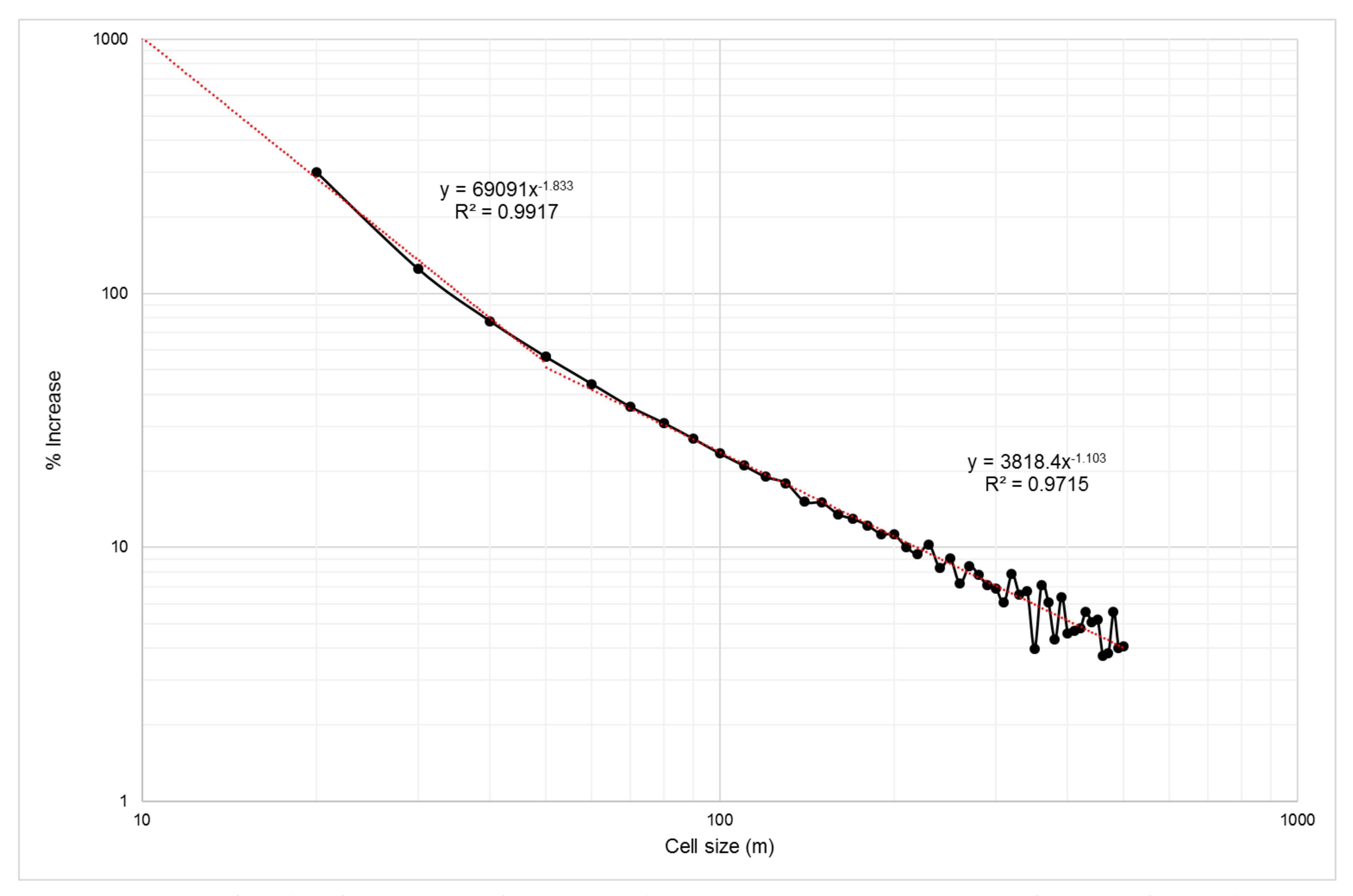
The geospatial dataset for this study is selected based on availability of the data and its usefulness to be used as proxy for our conceptual exploration model.

Geological data were derived from 1:50,000 British Columbia digital geology data compilation that was last updated on 5 April 2018 [36] (original dataset related to this article can be found at https://catalogue.data.gov.bc.ca/dataset/bedrock-geology, a public online data repository hosted at Data Catalogue by the Government of British Columbia; accessed on 25 March 2019). In the study area, Au-hydrothermal deposits are strongly correlated with intrusions from the Late Triassic-Early Jurassic and structurally controlled [34]. Therefore, we created predictor maps of distances to Texas Creek Plutonic Suite and Stikine Plutonic Suite intrusions and distance to fault traces at 500 m intervals. Moreover, reactive lithologies can act as a chemical trap for Au deposition. As such, reactive lithologies of the Stuhini Group and the Hazelton Group were categorized as ‘favorable’ host-rock while the other lithologies present in the study area were categorized as ‘non-favorable’ host-rock.

The geochemical data comes from a compiled database of soil samples from historic geochemical surveys conducted by private companies from 1981 to 2011. The elements analyzed and the analytical methods used in each survey varied and were not always adequately reported. Exploration efforts focused on areas surrounding known prospects, thus do not cover the entire study area. Only the twelve most present elements in the database were kept for further analysis: Ag, Au, As, Ba, Co, Cu, Fe, Mn, Mo, Pb, Sb, Zn. Values below the lower detection limit were replace by half the detection limit. No imputation was performed on the missing data. Hence, our geochemical dataset contains some missing data. The dataset was transformed using centered log-ratio (clr) [37]. Then, principal component analysis (PCA) is applied to the transformed dataset. Principal components can be interpreted as describing separate geological processes (i.e., differentiation, alteration, mineralization, weathering) [38]. In this study, only PC1 and PC2 were kept as the variation between the loadings of the different elements decreased as the number of principal components increased. They account for 34% and 14% of the variance respectively. Based on the loadings of the different elements (

Table 1. Rotated component matrix of principal component analysis of clr-transformed soil samples. Significant loadings (bolded values) are based on the absolute threshold of value 0.3.

	Ag	Au	As	Ba	Co	Cu	Fe	Mn	Mo	Pb	Sb	Zn
PC1	−0.41	−0.39	0.21	0.28	0.04	0.12	−0.26	0.35	−0.24	0.25	−0.29	0.39
PC2	0.09	0.28	0	0.21	0.1	−0.38	−0.38	0.40	−0.15	−0.46	−0.29	−0.30

), PC1 and PC2 seem to represent potential metal associations (e.g., Ag-Au-Sb), and enrichment or depletion. The clr-transformed Au values and the PC1 and PC2 were interpolated using the Inverse Distance Weighted (IDW) algorithm.

The geophysical data consists of magnetic data only, as it was the only available data in the area with a relatively small spatial resolution (200 m × 200 m) and was downloaded from the Canadian Aeromagnetic data base. Only processed data was available for download, and we chose to use the first vertical derivative as it is useful to enhance near-surface structure.

For remote sensing data, we used ASTER Level 1 Precision Terrain Corrected Registered At-Sensor Radiance (L1T) data, with a spatial resolution of 15 m, 30 m, and 90 m for the NIR, SWIR and TIR bands respectively. The SWIR and TIR band images were re-sampled to the VNIR band images resolution. The project study area is densely vegetated in the valleys but vegetation becomes scarce with altitude. The area is covered by snow from October to April with presence of multiple glaciers. In order to maximize bedrock exposure, we selected scenes acquired in summer to minimize snow cover and with minimum cloud cover (Figure 5). The ASTER data was atmospherically corrected and converted to relative reflectance using the Semi-Automatic Classification Plugin in QGIS software.

Hydrothermal alteration can effectively be mapped with ASTER data [39,40,41]. Band ratio (BR) and relative absorption band depth (RBD) methods are useful to enhance the absorption feature of some characteristic alteration minerals [42,43]. In this study, the following ratios to map the main alteration present in a hydrothermal system are used [44,45]:

$$Argilic=\frac{b4+b6}{b5}$$

(5)

$$Ironoxides=\frac{b4}{b2}$$

(6)

$$Phyllic=\frac{b5+b7}{b6}$$

(7)

$$Propylitic=\frac{b7+b9}{b8}$$

(8)

$$Silica=\frac{b11}{b12}$$

(9)

A total of twelve predictor maps are generated to map the mineral potential of epithermal Au in the study area (Figure 6 and Figure 7).

4.1.3. Cell Size

Using the methodology laid out by Carranza [46], the unit cell size is determined using point pattern analysis. First, the higher limit of a set of suitable cell size is determined by finding the distance where the likelihood of finding deposits located next to one another is null. That distance is 515 m. The lower limit depends on the predictor map with the smallest scale and can be estimated using the following formula [47]:

$$x=MS\times 0.00025,$$

(10)

where $MS$ is the map scale factor. In this study, the predictor maps were derived from 1:50,000 geological map and ASTER images (resolution of 15 m, 30 m, 90 m for the NIR, SWIR and TIR bands respectively). Thus, 12.5 m is the lower limit. The most suitable cell-size can be determined by fitting straight lines to the log-log plot of the rate of increase of the ratio $\left[N\right(D\left)\right]:\left[N\right(T)-N(D\left)\right]$ based on a cell-size to the next coarser cell-size, with $\left[N\right(T\left)\right]$ being the total number of cells and $\left[N\right(D\left)\right]$ being the number of cells containing one deposit [46]. The most suitable cell size for our study area is defined by the intersection of the two straight lines fitted to the log-log plot (Figure 8); thus, we selected a 50 m cell size.

4.2. RF Algorithm Parameters

As presented in Section 2, RF requires only two essential parameters: k and $m_{try}$. The k parameter represents the number of trees in the ensemble and $m_{try}$ is the number of input features selected to do the splitting at each node of a tree. In this study, various values of k (from 500 to 5000) and selected $k=1000$ as the generalization error started to converge from $k\ge 1000$. The lowest RMSE on the OOB samples was used to select the optimal value of $m_{try}$.

4.3. Model Evaluation

After optimization of the RF parameter, the performance of the best-fit models was comprehensively evaluated using confusion matrix, indices of predictive accuracy, and success-rate curves.

A series of statistical indices are calculated from the confusion matrix and permit to evaluate the predictive performance of the trained model:

$$Sensitivity=\frac{TP}{TP+FN}$$

(11)

$$Specificity=\frac{TN}{TN+FP}$$

(12)

$$Accuracy=\frac{TP+TN}{TP+TN+FP+FN}$$

(13)

$$Kappa=\frac{(TP+TN)-\frac{(TP+FN)(TP+FP)+(FP+TN)(FN+TN)}{(TP+FP+TN+FN)}}{(TP+FP+TN+FN)-\frac{(TP+FN)(TP+FP)+(FP+TN)(FN+TN)}{(TP+FP+TN+FN),}}$$

(14)

where TP is True Positive, TN is True Negative, FN is False Negative, and FP is False Positive.

The kappa index measures the fit between the predictor maps and the training dataset [48], the sensitivity and specificity indicate whether the deposit cells or non-deposit cells are correctly classified to their corresponding class respectively. Success-rate curves can be employed to evaluate the overall performance of the models. The curve is generated by calculating the percentage of correctly delineated training deposit in a prospective area for a given threshold with an increment of 5-percentile of the likelihood value [22].

5. Results

5.1. Relative Importance of Predictor Maps

As explained in Section 2, the RF algorithm measures the importance of each predictor maps which provides insights on the best proxies for mineralization in the study area (Figure 9).

Overall, the five most important predictors are PC2, intrusion, host rock, fault, and Au in respective order from higher to lower cumulated percentage. These features represent the principal components of any epithermal Au exploration: source, pathway, physical trap, and chemical trap.

The source of the mineralized hydrothermal fluids is represented by the proximity to porphyritic intrusive bodies of Late Triassic to Early Jurassic age. The faults correspond to the pathway taken by gold-bearing fluids and they can also act as physical traps for those fluids. Lithologies from the Stuhini and Hazelton Group can act as a chemical trap for mineralized fluids. Geochemical anomalies of Au and other pathfinder elements, represented by Au and PC2 predictor maps, are also proxies of a chemical trap.

Among the different hydrothermal alteration mapped using the ASTER images, the phyllic and silica alteration have the highest cumulated percentage.

5.2. Predictive Accuracy of the Model

The predicted values range between 0 and 1 and symbolize the probability of occurrence of Au mineral deposit. A threshold of 0.5 was used to classify predictions and to calculate the statistical indices in

Table 2. Accuracy of models generated with different sets of random point pattern NDL (R1 to R10).

	R1	R2	R3	R4	R5	R6	R7	R8	R9	R10
Accuracy	88%	67%	72%	78%	75%	81%	83%	83%	81%	72%
Kappa	78%	33%	44%	56%	50%	61%	67%	67%	61%	44%
Sensitivity	94%	61%	67%	78%	78%	78%	89%	83%	78%	67%
Specificity	83%	72%	78%	78%	72%	83%	78%	83%	83%	78%

and

Table 3. Accuracy of models generated with selected non-prospective KMO NDL and the mean and standard deviation of accuracy indices of models generated with different sets of random point pattern NDL.

	Selected	Mean	Sd
Accuracy	84%	78%	6%
Kappa	67%	56%	13%
Sensitivity	79%	77%	10%
Specificity	89%	79%	4%

. Cells with a value higher than the threshold are considered prospective, whereas values below the threshold are considered non-prospective.

The average accuracy of the random models is lower than the selected model, with 78% and 84%, respectively. The kappa values of 56% and 67% of the averaged random models and the selected model respectively indicate that both models have a moderate fit between the predictor maps and the training datasets [48].

Of all the random models, only R1 yields better results than the selected model, but overall, the selected model is more accurate than the random models. Although the results indicate that all models can capture the spatial relationship between the predictor maps and the training datasets, the selected model is the most accurate.

5.3. Performance of RF Modelling

In the previous section, the predictive accuracy of each model is reviewed. However, the models are not evaluated in a spatial context. For that purpose, success-rate curves, describing the performance of the RF modeling based on the resulting predictive maps, are used (Figure 10).

Of the eleven mineral prospectivity maps, the worst performing model is the R1 model which requires 35% of the study area to delineate all of the training deposits. In contrast, the best performing maps capture all of the training deposits in 15% of the study area. Those maps are obtained with the Sel, R6 and R9 models (Figure 11, Figure 12 and Figure 13).

6. Conclusions

In this study, different training sets using selected non-prospective KMO and ten sets of randomly generated non-deposit location are compared. The type of deposit could not be used as a selection criterion to select the KMO because the area is an extensive epithermal system. Hence, some of the non-prospective KMO can have a similar geospatial signature as our deposit training data set and introduce bias.

Across all the models, the five predictor maps with the highest cumulated relative importance are representative of the source, pathway, and both physical and chemical traps of an epithermal Au deposit. The different model predictive accuracy are compared and it is found that the model using selected non-prospective KMO has higher accuracy than the average accuracy of the models using random NDL with 84% and 78%, respectively. Thus, using the listed commodities as a discriminant to select non-prospective KMO is enough to have an accurate resulting model.

The predictive maps are evaluated using success-rate curves. The best mineral prospectivity maps are obtained with the R6, R9,and Sel training sets that capture 100% training deposits in 15% of the prospective area. Therefore, when available, it is recommended using KMO classified as ‘non-prospective’ for the commodity sought rather than the randomly generated non-deposit training set. However, for the larger study area were a diversity of deposit types is present, it is recommended to use the commodities and the deposit type as selection criteria to strengthen the predictive accuracy of the model further.

As found in this study, MPM using RF can be used in early stages of an exploration project when only public data are available. By analyzing and interpreting the response of the target variable to a set of predictor variables, RF is very similar to other knowledge-guided data-driven methods such as evidential belief and weights of evidence modeling. RF can also impute missing values, both continuous and categorical data, particularly when handling heterogeneous datasets, which is the case in this study. This yields an out-of-bag imputation error estimate without the need of a test set or elaborate cross-validation. These characteristics make RF a non-black-box exploration method, which is more suitable for mineral prospectivity modeling than other currently used machine learning approaches.

References

1. Bonham-Carter, G.F. Geographic Information Systems for Geoscientists: Modelling with GIS; Pergamon (Elsevier Science Ltd.): Oxford, UK, 1994. [Google Scholar]
2. Carranza, E.J.M. Geochemical Anomaly and Mineral Prospectivity Mapping in GIS. In Handbook of Exploration and Environmental Geochemistry, 2009th ed.; Elsevier Science: Amsterdam, The Netherlands, 2008; Volume 11. [Google Scholar]
3. Harris, J.; Grunsky, E.; Behnia, P.; Corrigan, D. Data- and knowledge-driven mineral prospectivity maps for Canada’s North. Ore Geol. Rev. 2015, 71, 788–803. [Google Scholar] [CrossRef]
4. Harris, J.; Wilkinson, L.; Heather, K.; Fumerton, S.; Bernier, M.A.; Ayer, J.; Dahn, R. Application of GIS Processing Techniques for Producing Mineral Prospectivity Maps—A Case Study: Mesothermal Au in the Swayze Greenstone Belt, Ontario, Canada. Nat. Resour. Res. 2001, 34, 91–124. [Google Scholar] [CrossRef]
5. Yousefi, M.; Carranza, E.J.M. Geometric average of spatial evidence data layers: A GIS-based multi-criteria decision-making approach to mineral prospectivity mapping. Comput. Geosci. 2015, 83, 72–79. [Google Scholar] [CrossRef]
6. Abedi, M.; Mostafavi Kashani, S.B.; Norouzi, G.H.; Yousefi, M. A deposit scale mineral prospectivity analysis: A comparison of various knowledge-driven approaches for porphyry copper targeting in Seridune, Iran. J. Afr. Earth Sci. 2017, 128, 127–146. [Google Scholar] [CrossRef]
7. Joly, A.; Porwal, A.; McCuaig, T.C. Exploration targeting for orogenic gold deposits in the Granites-Tanami Orogen: Mineral system analysis, targeting model and prospectivity analysis. Ore Geol. Rev. 2012, 48, 349–383. [Google Scholar] [CrossRef]
8. Porwal, A.; Das, R.D.; Chaudhary, B.; Gonzalez-Alvarez, I.; Kreuzer, O. Fuzzy inference systems for prospectivity modeling of mineral systems and a case-study for prospectivity mapping of surficial Uranium in Yeelirrie Area, Western Australia. Ore Geol. Rev. 2015, 71, 839–852. [Google Scholar] [CrossRef]
9. Yousefi, M.; Carranza, E.J.M. Fuzzification of continuous-value spatial evidence for mineral prospectivity mapping. Comput. Geosci. 2015, 74, 97–109. [Google Scholar] [CrossRef]
10. Yousefi, M.; Nykänen, V. Data-driven logistic-based weighting of geochemical and geological evidence layers in mineral prospectivity mapping. J. Geochem. Explor. 2016, 164, 94–106. [Google Scholar] [CrossRef]
11. Harris, D.; Zurcher, L.; Stanley, M.; Marlow, J.; Pan, G. A Comparative Analysis of Favorability Mappings by Weights of Evidence, Probabilistic Neural Networks, Discriminant Analysis, and Logistic Regression. Nat. Resour. Res. 2003, 12, 241–255. [Google Scholar] [CrossRef]
12. Porwal, A.; González-Álvarez, I.; Markwitz, V.; McCuaig, T.; Mamuse, A. Weights-of-evidence and logistic regression modeling of magmatic nickel sulfide prospectivity in the Yilgarn Craton, Western Australia. Ore Geol. Rev. 2010, 38, 184–196. [Google Scholar] [CrossRef]
13. Zhang, Z.; Zuo, R.; Xiong, Y. A comparative study of fuzzy weights of evidence and random forests for mapping mineral prospectivity for skarn-type Fe deposits in the southwestern Fujian metallogenic belt, China. Sci. China Earth Sci. 2016, 59, 556–572. [Google Scholar] [CrossRef]
14. Brown, W.M.; Gedeon, T.D.; Groves, D.I.; Barnes, R.G. Artificial neural networks: A new method for mineral prospectivity mapping. Aust. J. Earth Sci. 2000, 47, 757–770. [Google Scholar] [CrossRef]
15. Rodriguez-Galiano, V.F.; Sanchez-Castillo, M.; Chica-Olmo, M.; Chica-Rivas, M. Machine learning predictive models for mineral prospectivity: An evaluation of neural networks, random forest, regression trees and support vector machines. Ore Geol. Rev. 2015, 71, 804–818. [Google Scholar] [CrossRef]
16. Abedi, M.; Norouzi, G.H.; Bahroudi, A. Support vector machine for multi-classification of mineral prospectivity areas. Comput. Geosci. 2012, 46, 272–283. [Google Scholar] [CrossRef]
17. Geranian, H.; Tabatabaei, S.H.; Asadi, H.H.; Carranza, E.J.M. Application of Discriminant Analysis and Support Vector Machine in Mapping Gold Potential Areas for Further Drilling in the Sari-Gunay Gold Deposit, NW Iran. Nat. Resour. Res. 2016, 25, 145–159. [Google Scholar] [CrossRef]
18. Shabankareh, M.; Hezarkhani, A. Application of support vector machines for copper potential mapping in Kerman region, Iran. J. Afr. Earth Sci. 2017, 128, 116–126. [Google Scholar] [CrossRef]
19. Carranza, E.J.M.; Laborte, A.G. Data-driven predictive mapping of gold prospectivity, Baguio district, Philippines: Application of Random Forests algorithm. Ore Geol. Rev. 2015, 71, 777–787. [Google Scholar] [CrossRef]
20. Carranza, E.J.M.; Laborte, A.G. Data-Driven Predictive Modeling of Mineral Prospectivity Using Random Forests: A Case Study in Catanduanes Island (Philippines). Nat. Resour. Res. 2016, 25, 35–50. [Google Scholar] [CrossRef]
21. Hariharan, S.; Tirodkar, S.; Porwal, A.; Bhattacharya, A.; Joly, A. Random Forest-Based Prospectivity Modelling of Greenfield Terrains Using Sparse Deposit Data: An Example from the Tanami Region, Western Australia. Nat. Resour. Res. 2017, 26, 489–507. [Google Scholar] [CrossRef]
22. Rodriguez-Galiano, V.F.; Chica-Olmo, M.; Chica-Rivas, M. Predictive modelling of gold potential with the integration of multisource information based on random forest: A case study on the Rodalquilar area, Southern Spain. Int. J. Geogr. Inf. Sci. 2014, 28, 1336–1354. [Google Scholar] [CrossRef]
23. Carranza, E.J.M. Natural Resources Research Publications on Geochemical Anomaly and Mineral Potential Mapping, and Introduction to the Special Issue of Papers in These Fields. Nat. Resour. Res. 2017, 26, 379–410. [Google Scholar] [CrossRef]
24. Parsa, M.; Maghsoudi, A.; Yousefi, M. Spatial analyses of exploration evidence data to model skarn-type copper prospectivity in the Varzaghan district, NW Iran. Ore Geol. Rev. 2018, 92, 97–112. [Google Scholar] [CrossRef]
25. Sun, T.; Chen, F.; Zhong, L.; Liu, W.; Wang, Y. GIS-based mineral prospectivity mapping using machine learning methods: A case study from Tongling ore district, eastern China. Ore Geol. Rev. 2019, 109, 26–49. [Google Scholar] [CrossRef]
26. McKay, G.; Harris, J. Comparison of the Data-Driven Random Forests Model and a Knowledge-Driven Method for Mineral Prospectivity Mapping: A Case Study for Gold Deposits Around the Huritz Group and Nueltin Suite, Nunavut, Canada. Nat. Resour. Res. 2016, 25, 125–143. [Google Scholar] [CrossRef]
27. Zhang, S.; Xiao, K.; Carranza, E.J.M.; Yang, F. Maximum Entropy and Random Forest Modeling of Mineral Potential: Analysis of Gold Prospectivity in the Hezuo–Meiwu District, West Qinling Orogen, China. Nat. Resour. Res. 2019, 28, 645–664. [Google Scholar] [CrossRef]
28. Breiman, L. Random Forests. Mach. Learn. 2001, 5–32. [Google Scholar] [CrossRef] [Green Version]
29. Breiman, L. Bagging predictors. Mach. Learn. 1996, 24, 123–140. [Google Scholar] [CrossRef] [Green Version]
30. Breiman, L.; Friedman, J.H.; Olshen, R.A.; Stone, C.J. Classification And Regression Trees; Taylor & Francis Group: Boca Raton, FL, USA, 1984. [Google Scholar]
31. Macdonald, A.J.; Lewis, P.D.; Thompson, J.F.H.; Nadaraju, G.; Bartsch, R.; Bridge, D.J.; Rhys, D.A.; Roth, T.; Kaip, A.; Godwin, C.I.; et al. Metallogeny of an Early to Middle Jurassic arc, Iskut River area, northwestern British Columbia. Econ. Geol. 1996, 91, 1098–1114. [Google Scholar] [CrossRef]
32. Nelson, J.; Kyba, J. Structural and stratigraphic control of porphyry and related mineralization in the Treaty Glacier KSM Brucejack Stewart trend of western Stikinia. Br. Columbia Geol. Surv. Pap. 2014, 2013, 111–140. [Google Scholar]
33. Logan, J.M.; Mihalynuk, M.G. Tectonic Controls on Early Mesozoic Paired Alkaline Porphyry Deposit Belts (Cu-Au Ag-Pt-Pd-Mo) Within the Canadian Cordillera. Econ. Geol. 2014, 109, 827–858. [Google Scholar] [CrossRef]
34. Rhys, D.A. Geology of the Snip Mine and Its Relationship to the Magmatic and Deformational History of the Johnny Mountain Area, Northwestern British Columbia. Master’s Thesis, University of British Columbia, Vancouver, BC, Canada, 1993. [Google Scholar]
35. Rhys, D.A. Geology of the Stonehouse Gold Deposit (Johnny Mountain Gold Mine) and Exploration Implications; Technical Report; Spirit Bear Minerals Ltd.: Vancouver, BC, Canada, 1994. [Google Scholar]
36. Cui, Y.; Miller, D.; Schiarizza, P.; Diakow, L.J. British Columbia Digital Geology. In Open File 2017-8, British Columbia Ministry of Energy, Mines and Petroleum Resources; British Columbia Geological Survey: Victoria, BC, Canada, 2017. [Google Scholar]
37. Aitchison, J. The Statistical Analysis of Compositional Data; Chapman and Hall: London, UK, 1986. [Google Scholar]
38. Grunsky, E.C. The interpretation of geochemical survey data. Geochem. Explor. Environ. Anal. 2010, 10, 27–74. [Google Scholar] [CrossRef]
39. Crósta, A.P.; De Souza Filho, C.R.; Azevedo, F.; Brodie, C. Targeting key alteration minerals in epithermal deposits in Patagonia, Argentina, using ASTER imagery and principal component analysis. Int. J. Remote Sens. 2003, 24, 4233–4240. [Google Scholar] [CrossRef]
40. Di Tommaso, I.; Rubinstein, N. Hydrothermal alteration mapping using ASTER data in the Infiernillo porphyry deposit, Argentina. Ore Geol. Rev. 2007, 32, 275–290. [Google Scholar] [CrossRef]
41. Moore, F.; Rastmanesh, F.; Asadi, H.; Modabberi, S. Mapping mineralogical alteration using principal-component analysis and matched filter processing in the Takab area, north-west Iran, from ASTER data. Int. J. Remote Sens. 2008, 29, 2851–2867. [Google Scholar] [CrossRef]
42. Crowley, J.K.; Brickey, D.W.; Rowan, L.C. Airborne imaging spectrometer data of the Ruby Mountains, Montana: Mineral discrimination using relative absorption band-depth images. Remote Sens. Environ. 1989, 29, 121–134. [Google Scholar] [CrossRef]
43. Rowan, L.C.; Mars, J.C. Lithologic mapping in the Mountain Pass, California area using Advanced Spaceborne Thermal Emission and Reflection Radiometer (ASTER) data. Remote Sens. Environ. 2003, 84, 350–366. [Google Scholar] [CrossRef]
44. Pour, A.B.; Hashim, M. Identification of hydrothermal alteration minerals for exploring of porphyry copper deposit using ASTER data, SE Iran. J. Asian Earth Sci. 2011, 42, 1309–1323. [Google Scholar] [CrossRef]
45. Rajendran, S.; Nasir, S. Characterization of ASTER spectral bands for mapping of alteration zones of volcanogenic massive sulphide deposits. Ore Geol. Rev. 2017, 88, 317–335. [Google Scholar] [CrossRef]
46. Carranza, E.J.M. Objective selection of suitable unit cell size in data-driven modeling of mineral prospectivity. Comput. Geosci. 2009, 35, 2032–2046. [Google Scholar] [CrossRef]
47. Hengl, T. Finding the right pixel size. Comput. Geosci. 2006, 32, 1283–1298. [Google Scholar] [CrossRef]
48. Landis, J.R.; Koch, G.G. The Measurement of Observer Agreement for Categorical Data. Biometrics 1977, 33, 159. [Google Scholar] [CrossRef] [PubMed] [Green Version]
Figure 1. Workflow of the random forest algorithm.
Minerals 11 00597 g001
Figure 2. Regional geology of the Iskut River area with the study area outlined in black from BC digital geology data repository.
Minerals 11 00597 g002
Figure 3. Result of point pattern analysis showing probability of finding another Au deposit from any given deposit for different distances.
Minerals 11 00597 g003
Figure 4. Location of deposits showing the buffer zone (in grey).
Minerals 11 00597 g004
Figure 5. False color ASTER image derived from Band 2, Band 4 and Band 7 as RGB color combination showing the glacier and water (blue), vegetation (green) and exposed bedrock and sediments (yellow).
Minerals 11 00597 g005
Figure 6. Predictor maps of (a) distance to intrusions, (b) distance to fault, (c) favorable host-rock, (d) Au geochemical anomaly, (e) PC1, and (f) PC2.
Minerals 11 00597 g006aMinerals 11 00597 g006b
Figure 7. Predictor maps of (a) magnetic first vertical derivative, (b) argillic alteration, (c) iron oxides alteration, (d) phyllic alteration, (e) propylitic alteration and (f) silica alteration.
Minerals 11 00597 g007aMinerals 11 00597 g007b
Figure 8. L o g l o g plot of rates (in %) of increase in the ratio [ N ( D ) ] : [ N ( T ) N ( D ) ] as a function of unit cell size.
Minerals 11 00597 g008
Figure 9. Sum of the relative importance percentage of each predictor map from models generated with different set of random point pattern non-deposit location (R1 to R10) and selected non-prospective KMO (Sel).
Minerals 11 00597 g009
Figure 10. Success-rate curves of predictive map of Au prospectivity obtained by using training set with random non-deposit location (R1–R10) and with selected non-prospective KMO.
Minerals 11 00597 g010
Figure 11. Mineral prospectivity map with Sel model (a) and delineated prospective area (b).
Minerals 11 00597 g011
Figure 12. Mineral prospectivity map with R6 model (a) and delineated prospective area (b).
Minerals 11 00597 g012
Figure 13. Mineral prospectivity map with R9 model (a) and delineated prospective area (b).
Minerals 11 00597 g013