
Investigation of Error Distribution in the Back-Calculation of Breakage Function Model Parameters via Nonlinear Programming


Abstract
:1. Introduction
2. Materials and Methods
2.1. Methodology
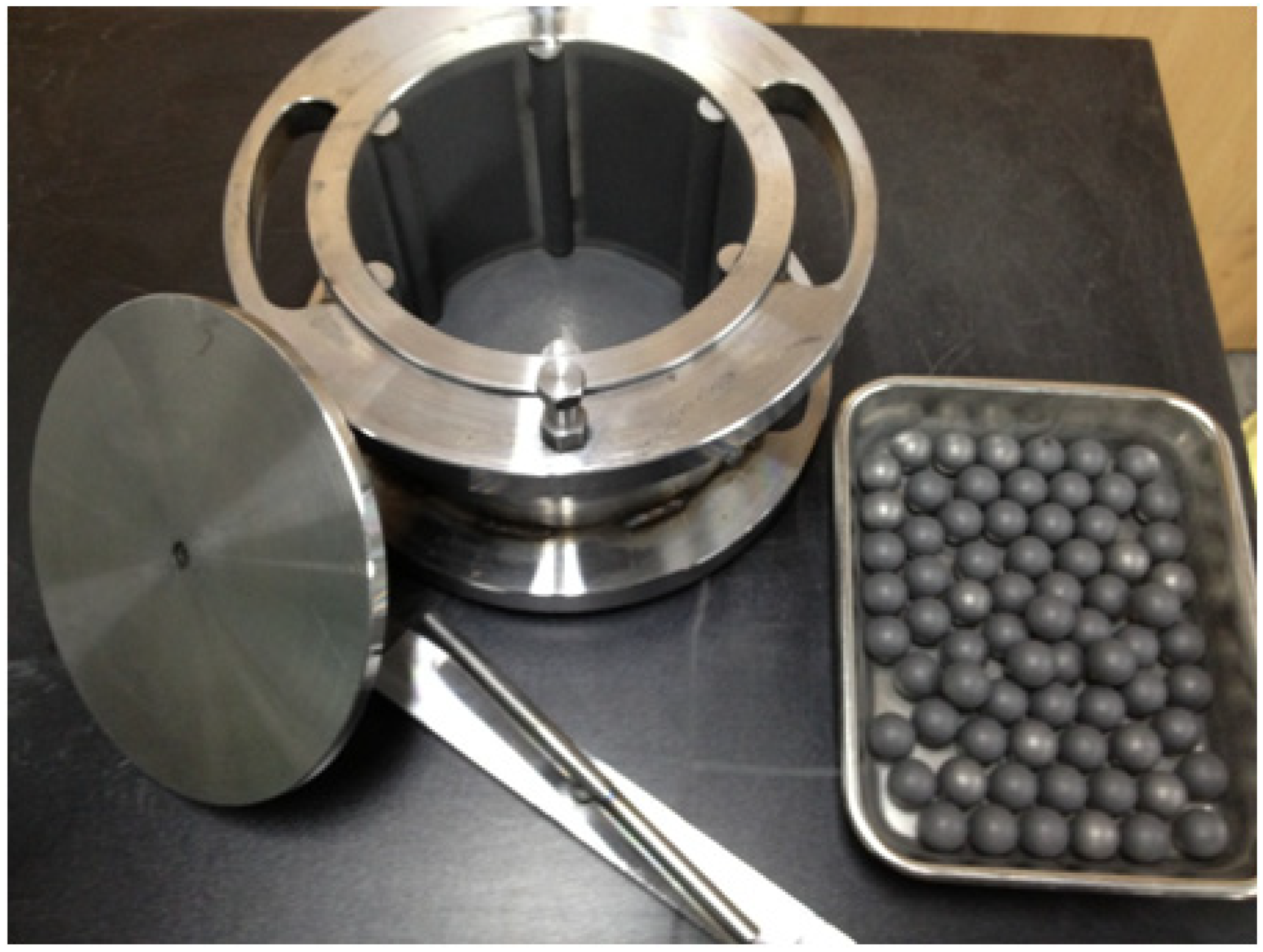
2.2. Experimental
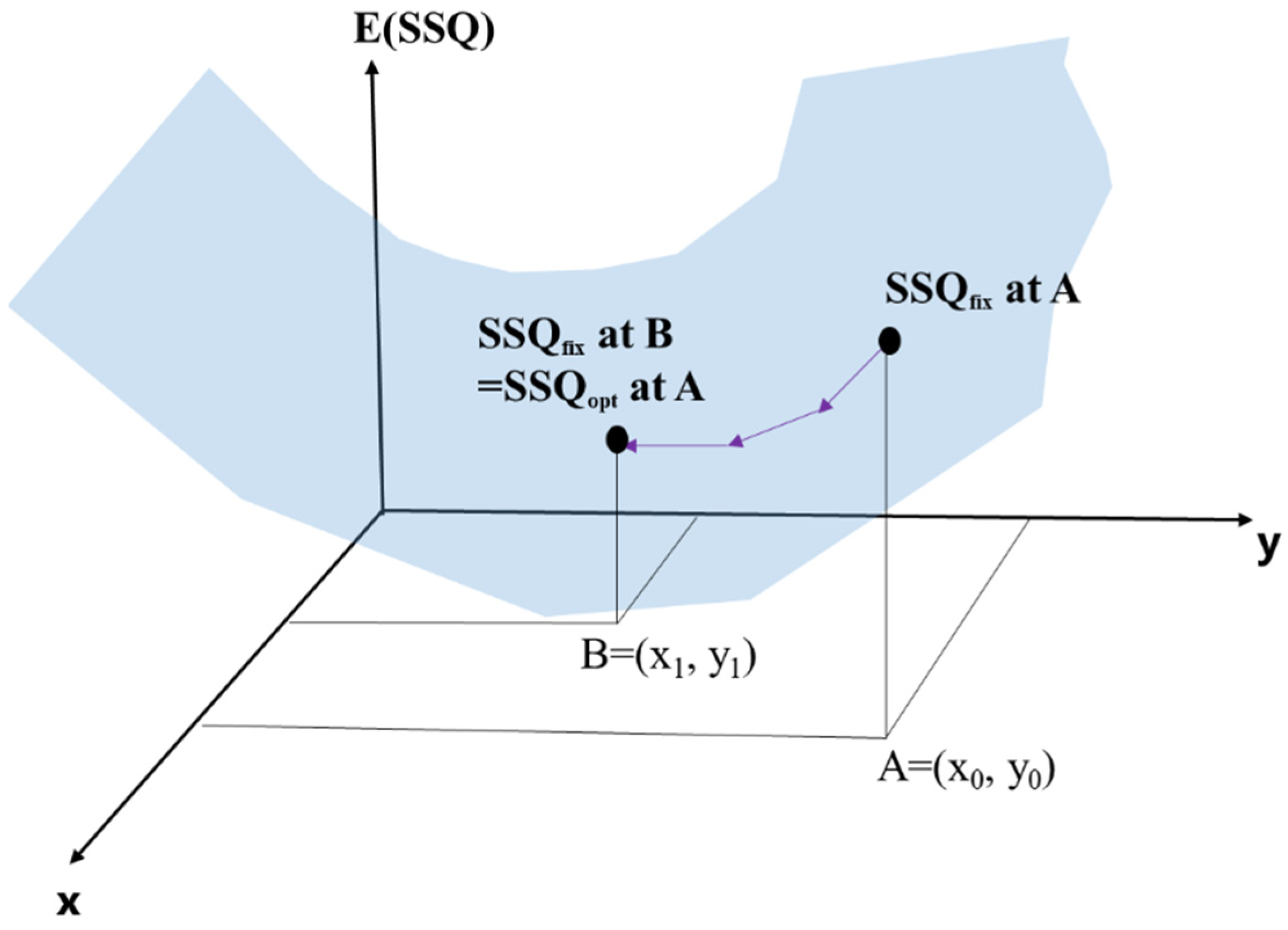
2.3. Back-Calculation and Analysis
3. Result and Discussion
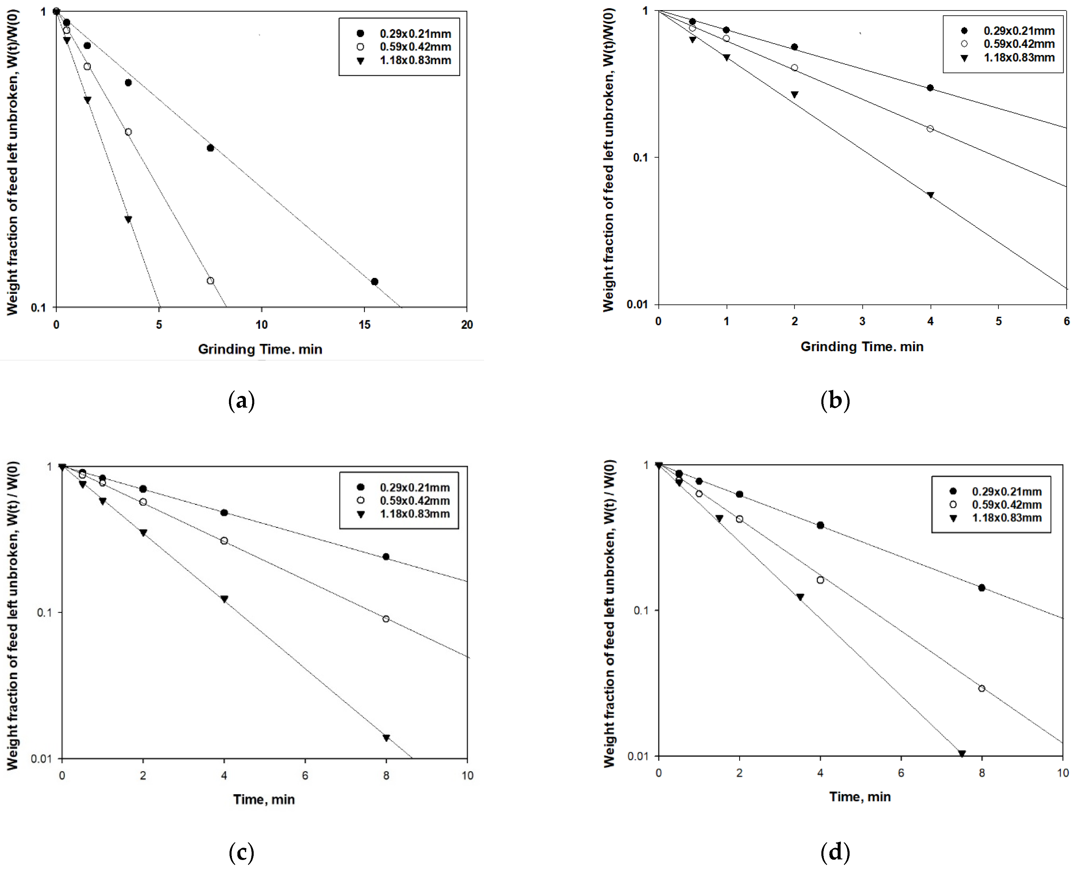
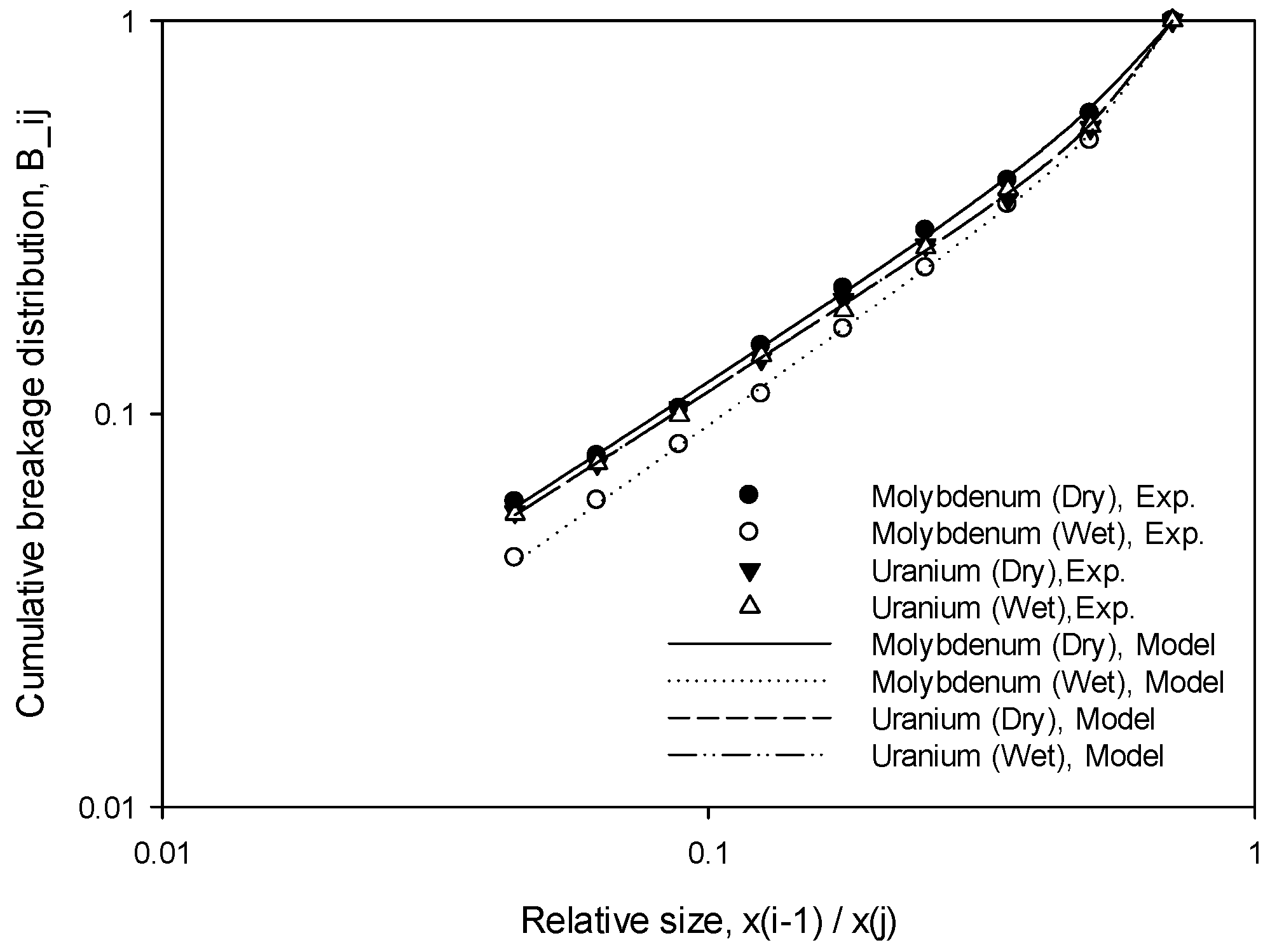
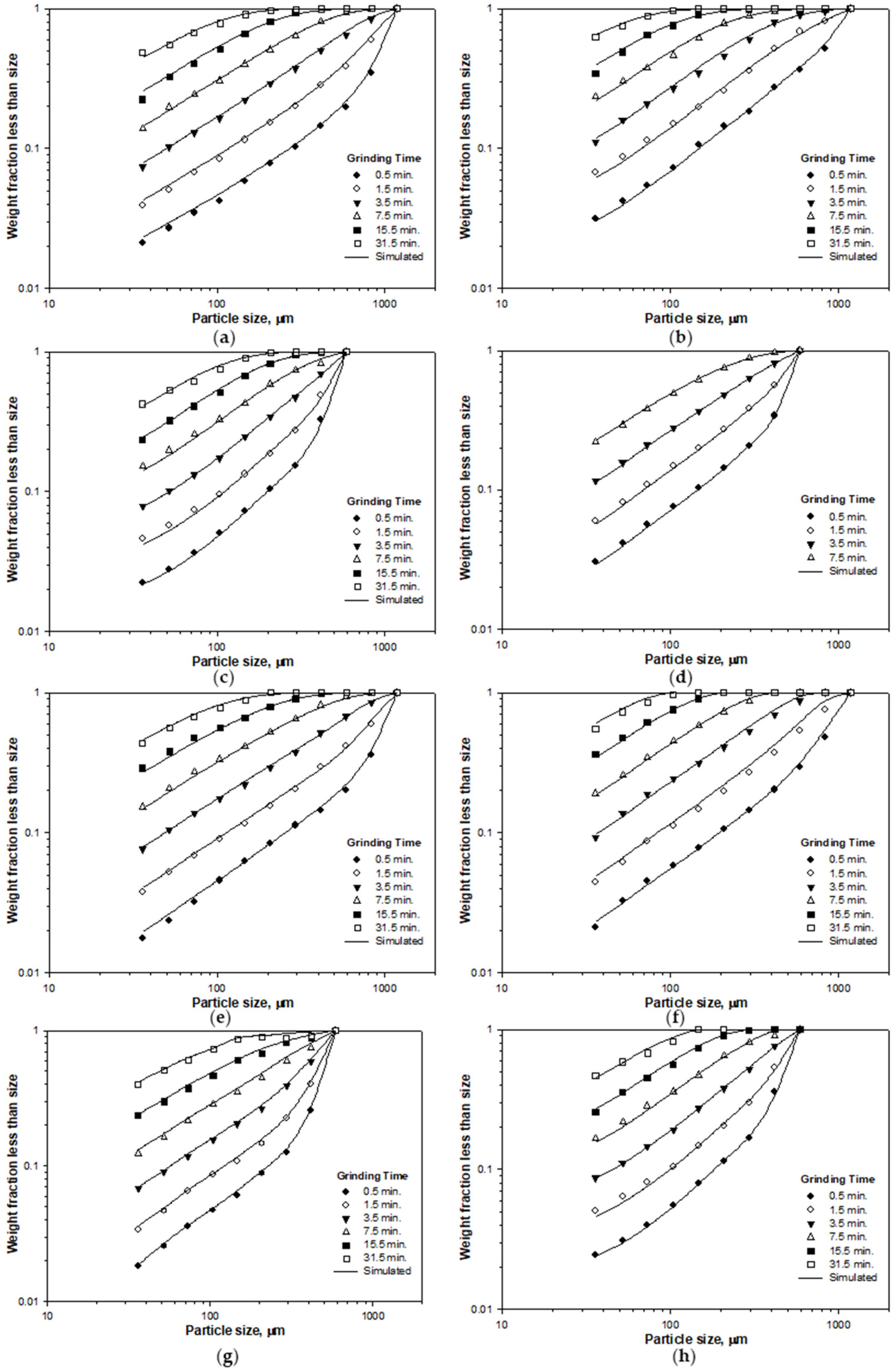
3.1. Experimental (Breakage Parameters from SSFBTs)
3.2. Back-Calculation: Error Function Distribution Analysis
4. Conclusions
- (1)
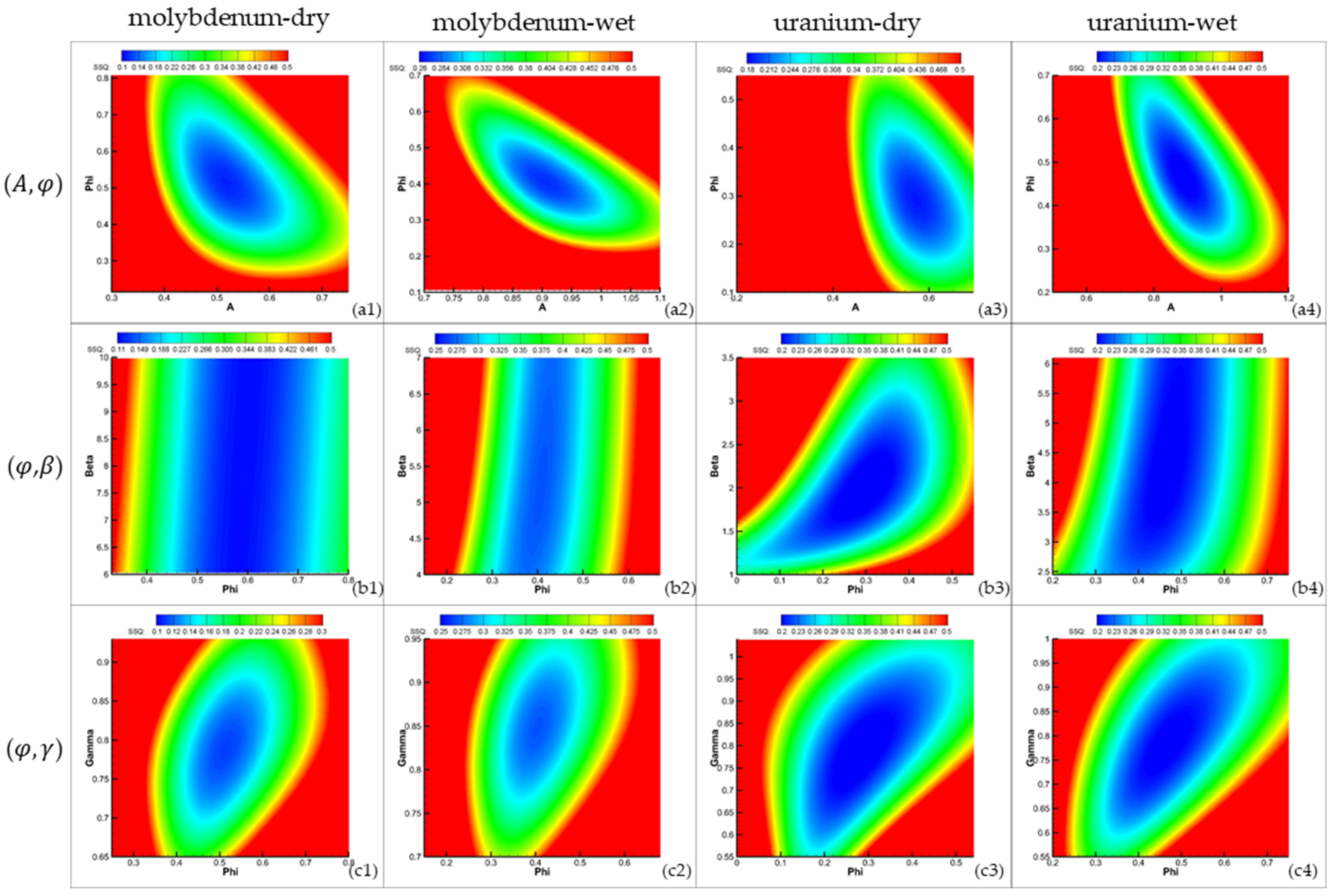
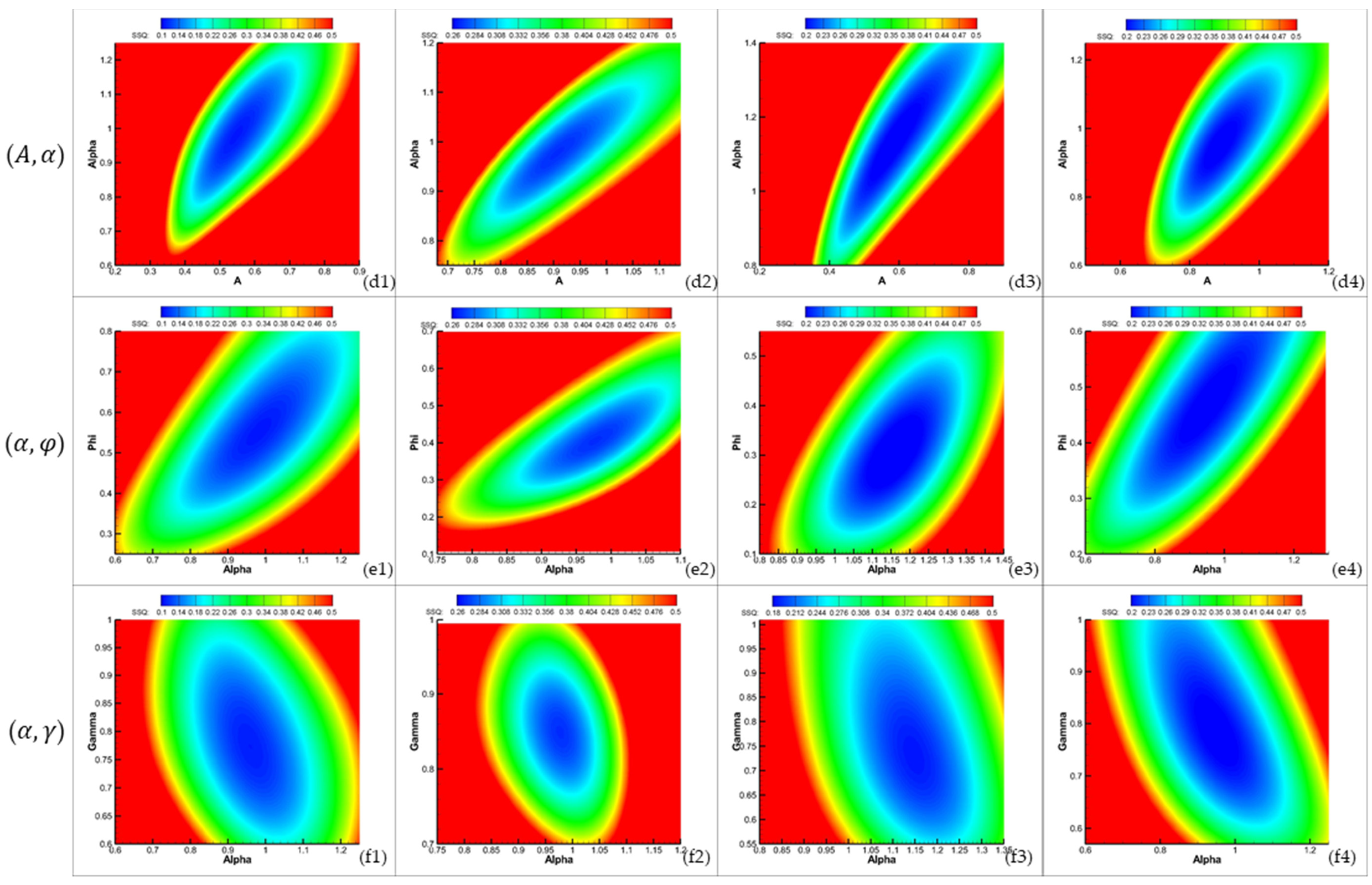
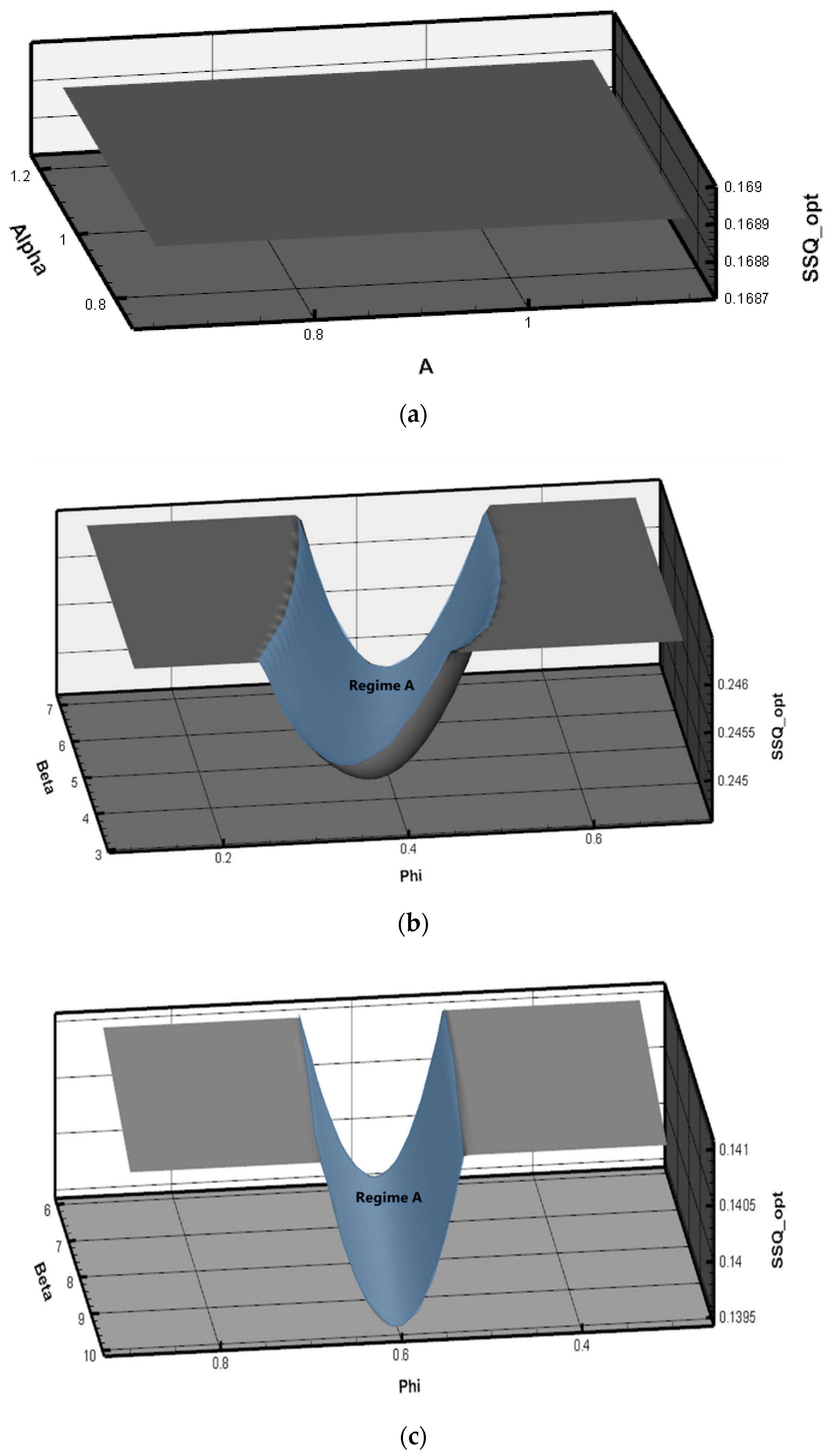
- In the two-dimensional parameter space, the error function was strictly convex, and no local minima differing from the global minima were observed. The main problem during back-calculation of the breakage parameters was weak convergence owing to the flat surface of the error function rather than occurrence of local minima. For molybdenum grinding, the shape of the error function for the (φ, β) pair was flatter compared to that for other parameter pairs. We attributed this to the strong mutual interference between these two parameters.
- (2)
- In the back-calculation involving the two-dimensional parameter space, for most pairs of variables, the optimization process converged to a single point and the results agreed well with those obtained through SSFBTs. However, for the parameter space with the pair producing a flat error function distribution, the solution of the back-calculation failed to converge.
- (3)
- Through wide-range search, even when convergence failed, the parameter combination that produced the minimum error agreed well with the parameters obtained from the SSFBTs. Thus, we could successfully determine the BFPs through wide-range search, irrespective of the shape of the error function.
- (4)
- Wide-range search proved feasible for searching in the three-dimensional parameter space, irrespective of the choice of parameters. For four- or five-dimensional parameter spaces, the accuracy of the back-calculation method decreased depending on the parameters that had to be back-calculated.
- (5)
- In conclusion, without proper initial values, searching seven breakage parameters through back-calculation only is not recommended owing to accuracy problems. When the number of parameters to be back-calculated is not greater than four, the parameters could be accurately identified through wide-range search, indicating that the number of SSFBTs required to determine the breakage function can be effectively reduced using the wide-range search.
Author Contributions
Funding
Data Availability Statement
Acknowledgments
Conflicts of Interest
References
- Napier-Mun, T. Is progress in energy-efficient comminution doomed? Miner. Eng. 2015, 73, 1–6. [Google Scholar] [CrossRef]
- Austin, L.G.; Klimpel, R.R.; Luckie, P.T. Process Engineering of Size Reduction: Ball Milling; Society of Mining Engineers of the American Institute of Mining, Metallurgical, and Petroleum Engineers: New York, NY, USA, 1984. [Google Scholar]
- Rittinger, R.P.V. Lehrbuch der Aufbereitungskunde; Ernst and Korn: Berlin, Germany, 1867. [Google Scholar]
- Kick, F. Das Gesetz der Proportionalen Widerstande und Seine Anwendung Felix; Verlag Von Arthur Felix: Leipzig, Germany, 1885. [Google Scholar]
- Bond, F.C. The third theory of comminution. Trans. AIME 1952, 193, 484–494. [Google Scholar]
- Austin, L.G.; Luckie, P.T. Methods for determination of breakage distribution parameters. Powder Technol. 1972, 5, 215–222. [Google Scholar] [CrossRef]
- Austin, L.G.; Luckie, P.T. The estimation of non-normalized breakage distribution parameters from batch grinding tests. Powder Technol. 1972, 5, 267–270. [Google Scholar] [CrossRef]
- Luckie, P.T.; Austin, L.G. A Review introduction to the solution of the grinding equations by digital computation. Miner. Sci. Eng. 1972, 4, 24–51. [Google Scholar]
- Reid, K.J. A solution to the batch grinding equation. Chem. Eng. Sci. 1965, 20, 953–963. [Google Scholar] [CrossRef]
- Mishra, B.K.; Rajamani, R.K. The discrete element method for the simulation of ball mills. Appl. Math. Model. 1992, 16, 598–604. [Google Scholar] [CrossRef]
- Cleary, P.W.; Sinnot, M.; Morrison, R. Prediction of slurry transport in SAG mills using SPH fluid flow in a dynamic DEM based porous media. Miner. Eng. 2006, 19, 1517–1527. [Google Scholar] [CrossRef]
- Cleary, P.W. Charge behaviour and power consumption in ball mills, sensitivity to mill operating conditions, liner geometry and charge composition. Int. J. Miner. Process. 2001, 63, 79–114. [Google Scholar] [CrossRef]
- Metta, N.; Ierapetritou, M.; Ramachandran, R. A multiscale DEM-PBM approach for a continuous comilling process using a mechanistically developed breakage kernel. Chem. Eng. Sci. 2018, 178, 211–221. [Google Scholar] [CrossRef]
- Tuzcu, E.T.; Rajamani, R.K. Modeling breakage rates in mills with impact energy spectra and ultra fast load cell data. Miner. Eng. 2011, 24, 252–260. [Google Scholar] [CrossRef]
- Bnà, S.; Ponzini, R.; Cestari, M.; Cavazzoni, C.; Cottini, C.; Benassi, A. Investigation of particle dynamics and classification mechanism in a spiral jet mill through computational fluid dynamics and discrete element methods. Powder Technol. 2020, 364, 746–773. [Google Scholar] [CrossRef]
- Kwon, J.; Kim, H.; Lee, S.; Cho, H. Simulation of particle-laden flow in a Humphrey spiral concentrator using dust-liquid smoothed particle hydrodynamics. Adv. Powder Technol. 2017, 28, 2694–2705. [Google Scholar] [CrossRef]
- Napier-Munn, T.J.; Morrell, S.; Morrison, R.D.; Kojovic, T. Mineral Comminution Circuits: Their Operation and Optimisation; Julius Kruttschnitt Mineral Research Centre: Indooroopilly, Australia, 1996. [Google Scholar]
- Narayanan, S.S.; Whiten, W.J. Breakage characteristics of ores for ball mill modelling. Proc. Australas. Institut. Min. Metall. 1983, 286, 31–39. [Google Scholar]
- Whiten, W.J. A matrix theory of comminution machines. Chem. Eng. Sci. 1974, 29, 31–34. [Google Scholar] [CrossRef]
- Shi, F.; Xie, W. A specific energy-based ball mill model: From batch grinding to continuous operation. Miner. Eng. 2016, 86, 66–74. [Google Scholar] [CrossRef]
- Shi, F.; Xie, W. A specific energy-based size reduction model for batch grinding ball mill. Miner. Eng. 2015, 70, 130–140. [Google Scholar] [CrossRef]
- Shi, F.; Kojovic, T.; Brennan, M. Modelling of vertical spindle mills. Part 1: Sub-models for comminution and classification. Fuel 2015, 143, 595–601. [Google Scholar] [CrossRef]
- Shi, F.N.; Kojovic, T.; Esterle, J.S.; David, D. An energy-based model for swing hammer mills. Int. J. Miner. Process. 2003, 71, 147–166. [Google Scholar] [CrossRef]
- Deniz, V. The effects of ball filling and ball diameter on kinetic breakage parameters of barite powder. Adv. Powder Technol. 2012, 23, 640–646. [Google Scholar] [CrossRef]
- Austin, L.G. A discussion of equations for the analysis of batch grinding data. Powder Technol. 1999, 106, 71–77. [Google Scholar] [CrossRef]
- Kwon, J. Simulation and optimization of a two-stage ball mill grinding circuit of molybdenum ore. Adv. Powder Technol. 2016, 27, 1073–1085. [Google Scholar] [CrossRef]
- Lee, H.; Klima, M.S.; Saylor, P. Evaluation of a laboratory rod mill when grinding bituminous coal. Fuel 2012, 92, 116–121. [Google Scholar] [CrossRef]
- Kwon, J.; Cho, H.; Mun, M.; Kim, K. Modeling of coal breakage in a double-roll crusher considering the reagglomeration phenomena. Powder Technol. 2012, 232, 113–123. [Google Scholar] [CrossRef]
- Kwon, J. Investigation of breakage characteristics of low rank coals in a laboratory swing hammer mill. Powder Technol. 2014, 256, 377–384. [Google Scholar] [CrossRef] [Green Version]
- Klimpel, R.R.; Austin, L.G. The back-calculation of specific rates of breakage from continuous mill data. Powder Technol. 1984, 38, 77–91. [Google Scholar] [CrossRef]
- Klima, M.S.; Luckie, P.T. Using model discrimination to select a mathematical function for generating separation curves. Coal Prep. 1986, 3, 33–47. [Google Scholar] [CrossRef]
- Gotsis, C.; Austin, L.G.; Luckie, P.T.; Shoji, K. Modeling of a grinding circuit with a swing-hammer mill and a twin-cone classifier. Powder Technol. 1985, 42, 209–216. [Google Scholar] [CrossRef]
- Austin, L.G.; Tangsathitkulchai, C. Comparison of methods for sizing ball mills using open-circuit wet grinding of phosphate ore as a test example. Ind. Eng. Chem. Res. 1987, 26, 997–1003. [Google Scholar] [CrossRef]
- Rogers, R.S.C.; Austin, L.G. Residence time distribution in ball mills. Part Sci. Technol. 1984, 2, 191–209. [Google Scholar] [CrossRef]
- Herbst, J.A.; Fuerstenau, D.W. Scale-up procedure for continuous grinding mill design using population balance models. Int. J. Miner. Process. 1980, 7, 1–31. [Google Scholar] [CrossRef]
- Avriel, M. Nonlinear Programming: Analysis and Methods; Prentice-Hall Inc.: Englewood Cliffs, NJ, USA, 1976. [Google Scholar]
- Dauphin, Y.N.; Pascanu, R.; Gulcehre, C.; Cho, K.; Ganguli, S.; Bengio, Y. Identifying and attacking the saddle point problem in high-dimensional non-convex optimization. arXiv 2014, arXiv:1406.2572. [Google Scholar]


| Parameter | Value | Unit |
|---|---|---|
| Mill Diameter, D | 200 | mm |
| Mill Depth, H | 165 | mm |
| Ball Loading, J | 0.2 | - |
| Powder Loading, U | 0.5 | - |
| Feed Size | 1180 × 834, 590 × 417, and 295 × 209 | μm2 |
| Grinding Time | 0.5, 1.5, 3.5, 7.5, 15.5, and 31.5 | min |
| Rotation speed | 0.75 | Φc |
| Parameters | Molybdenum | Uranium | ||
|---|---|---|---|---|
| Dry | Wet | Dry | Wet | |
| A | 0.5212 | 0.9064 | 0.5829 | 0.8856 |
| α | 0.9288 | 0.9767 | 1.1305 | 0.9504 |
| φ | 0.5155 | 0.4059 | 0.2599 | 0.4668 |
| γ | 0.7872 | 0.8490 | 0.7941 | 0.7827 |
| β | 8.0163 | 5.1306 | 1.8964 | 4.2609 |
| Molybdenum, Dry | |||||||
| SSFBT | 2D back-calculation | ||||||
| (A,φ) | (φ,β) | (φ,γ) | (A,α) | (α,φ) | (α,γ) | ||
| A | 0.5212 | 0.5226 | - | - | 0.5210 | - | - |
| α | 0.9288 | - | - | - | 0.9220 | 0.9213 | 0.9227 |
| φ | 0.5155 | 0.5132 | 0.5160 | 0.5165 | - | 0.5142 | - |
| γ | 0.7872 | - | - | 0.7807 | - | - | 0.7899 |
| β | 8.0163 | - | 8.0773 | - | - | - | - |
| Molybdenum, Wet | |||||||
| SSFBT | 2D back-calculation | ||||||
| (A,φ) | (φ,β) | (φ,γ) | (A,α) | (α,φ) | (α,γ) | ||
| A | 0.9064 | 0.9047 | - | - | 0.8997 | - | - |
| α | 0.9767 | - | - | - | 0.9746 | 0.9786 | 0.9733 |
| φ | 0.4059 | 0.4048 | 0.4045 | 0.4019 | - | 0.4093 | - |
| γ | 0.849 | - | - | 0.8541 | - | - | 0.8460 |
| β | 5.1306 | - | 5.1705 | - | - | - | - |
| Uranium, Dry | |||||||
| SSFBT | 2D back-calculation | ||||||
| (A,φ) | (φ,β) | (φ,γ) | (A,α) | (α ,φ) | (α ,γ) | ||
| A | 0.5829 | 0.5643 | - | - | 0.5751 | - | - |
| α | 1.1305 | - | - | - | 1.1171 | 1.0936 | 1.1675 |
| φ | 0.2599 | 0.2539 | 0.2648 | 0.2527 | - | 0.2652 | - |
| γ | 0.7941 | - | - | 0.7852 | - | - | 0.7774 |
| β | 1.8964 | - | 1.9416 | - | - | - | - |
| Uranium, Wet | |||||||
| SSFBT | 2D back-calculation | ||||||
| (A,φ) | (φ,β ) | (φ,γ ) | (A,α ) | (α ,φ) | (α ,γ) | ||
| A | 0.8856 | 0.9053 | - | - | 0.8728 | - | - |
| α | 0.9504 | - | - | - | 0.9775 | 0.9308 | 0.9339 |
| φ | 0.4668 | 0.4696 | 0.4685 | 0.4505 | - | 0.483 | - |
| γ | 0.7827 | - | - | 0.8009 | - | - | 0.8012 |
| β | 4.2609 | - | 4.2035 | - | - | - | - |
| 3D Back-Calculation | 4D Back-Calculation | 5D Back-Calculation | ||||||||||||||
|---|---|---|---|---|---|---|---|---|---|---|---|---|---|---|---|---|
| SSFBT | (A,α,φ) | (A,α,γ) | (A,α,β) | (A,φ,γ) | (A,φ,β) | (A,γ,β) | (α,φ,γ) | (α,φ,β) | (φ,γ,β) | (A,α,φ,γ) | (A,α,φ,β) | (A,α,γ,β) | (A,φ,γ,β) | (α,φ,γ,β) | (A,α,φ,γ,β) | |
| A | 0.5212 | 0.5294 | 0.5290 | 0.5285 | 0.5134 | 0.5299 | 0.5188 | - | - | - | 0.5209 | 0.5070 | 0.5162 | 0.5196 | - | 0.5072 |
| α | 0.9288 | 0.9155 | 0.9376 | 0.9314 | - | - | - | 0.9216 | 0.9227 | - | 0.9285 | 0.9337 | 0.9264 | - | 0.9287 | 0.9373 |
| φ | 0.5155 | 0.5200 | - | - | 0.5156 | 0.5465 | - | 0.5057 | 0.5435 | 0.5215 | 0.5159 | 0.4404 | - | 0.5058 | 0.5227 | 0.4706 |
| γ | 0.7872 | - | 0.7740 | - | 0.7783 | - | 0.7736 | 0.7859 | - | 0.7809 | 0.7896 | 0.7757 | 0.7769 | 0.7983 | 0.7049 | |
| β | 8.0163 | - | - | 7.9771 | - | 6.9436 | 7.9390 | - | 7.6987 | 7.7599 | - | 4.1241 | 6.7057 | 7.0245 | 9.0140 | 3.8323 |
| SSQopt | 0.1398 | 0.1558 | 0.1491 | 0.1476 | 0.1371 | 0.1492 | 0.1517 | 0.1405 | 0.1376 | 0.154 | 0.1421 | 0.1429 | 0.1406 | 0.1508 | 0.1503 | 0.1297 |
Publisher’s Note: MDPI stays neutral with regard to jurisdictional claims in published maps and institutional affiliations. |
© 2021 by the authors. Licensee MDPI, Basel, Switzerland. This article is an open access article distributed under the terms and conditions of the Creative Commons Attribution (CC BY) license (https://creativecommons.org/licenses/by/4.0/).
Share and Cite
Kwon, J.; Cho, H. Investigation of Error Distribution in the Back-Calculation of Breakage Function Model Parameters via Nonlinear Programming. Minerals 2021, 11, 425. https://doi.org/10.3390/min11040425
Kwon J, Cho H. Investigation of Error Distribution in the Back-Calculation of Breakage Function Model Parameters via Nonlinear Programming. Minerals. 2021; 11(4):425. https://doi.org/10.3390/min11040425
Chicago/Turabian StyleKwon, Jihoe, and Heechan Cho. 2021. "Investigation of Error Distribution in the Back-Calculation of Breakage Function Model Parameters via Nonlinear Programming" Minerals 11, no. 4: 425. https://doi.org/10.3390/min11040425